Costs and Benefits of Popular P-Value Correction Methods in Three Models of Quantitative Omic Experiments

Abstract

The multiple hypothesis testing problem is inherent in large-scale quantitative “omic” experiments such as mass spectrometry-based proteomics. Yet, tools for comparing the costs and benefits of different p-value correction methods under different experimental conditions are lacking. We performed thousands of simulations of omic experiments under a range of experimental conditions and applied correction using the Benjamini-Hochberg (BH), Bonferroni, and permutation-based false discovery proportion (FDP) estimation methods. The tremendous false discovery rate (FDR) benefit of correction was confirmed in a range of different contexts. No correction method can guarantee a low FDP in a single experiment, but the probability of a high FDP is small when a high number and proportion of corrected p-values are significant. On average, correction decreased sensitivity, but the sensitivity costs of BH and permutation were generally modest compared to the FDR benefits. In a given experiment, observed sensitivity was always maintained or decreased by BH and Bonferroni, whereas it was often increased by permutation. Overall, permutation had better FDR and sensitivity than BH. We show how increasing sample size, decreasing variability, or increasing effect size can enable the detection of all true changes while still correcting p-values, and we present basic guidelines for experimental design. Analysis of an experimental proteomic data set with defined changes corroborated these trends. We developed an R Shiny web application for further exploration and visualization of these models which we call the Simulator of P-value Multiple Hypothesis Correction (SIMPLYCORRECT) and a high-performance R package, permFDP, for easy use of the permutation-based FDP estimation method.

Introduction

It is now widely appreciated that many biological results are not reproducible.¹ Although the sources of irreproducibility vary, virtually all areas of biology suffer to some degree. In studies using analytical chemistry techniques that measure many analytes at once, such as mass spectrometry-based proteomics, the multiple hypothesis testing problem can produce an entire set of irreproducible results if not addressed.²

In quantitative omic experiments, researchers are often looking for differences. For example, in order to find new diagnostics or therapeutic targets for Alzheimer’s disease, proteomic studies screen for differences in protein abundances between Alzheimer’s disease patients and healthy controls.³ In such omic studies, m analytes (e.g., proteins, metabolites, or transcripts) are measured and the null hypothesis H_0i is tested against the alternative hypothesis H_Ai for each i^th analyte, where i ranges from 1 to m:

$$H_{0i}:\text{The }{i}^{\text{th}}\text{ analyte does not differ}.$$

$$H_{Ai}:\text{The} i^{\text{th}}\text{ analyte differs}.$$

When the T test is used, as is common in mass spectrometry, H_0i states specifically that the means of the underlying distributions are equal, while H_Ai states that the means are unequal.

With large m, the probability of a false positive (rejecting true H_0i) is high without correcting for multiple hypothesis testing. Usually, H_0i is rejected when the p-value (p_i) is below a threshold α (e.g., 0.05); in such cases, a dataset with zero true differences (i.e., all H_0i are actually true) will typically contain $m*\alpha$ “statistically significant” false hits if no correction is applied.⁴ This is the multiple hypothesis testing problem. Several methods have been developed to address this issue and are routinely used.^5,6 However, lists of uncorrected p-values still appear. In situations where uncorrected hits are presented and are not validated with targeted follow-up experiments, the results can be cited to support false claims.

Some researchers may be concerned that correction will decrease sensitivity (the proportion of true H_Ai identified) which can indeed occur. Incentivizes to maximize sensitivity may have limited the adoption of multiple hypothesis correction.⁷ In addition, some researchers may lack a sense of the costs and benefits of correcting omic data using different methods.

Many authors have assessed the effectiveness and limitations of correction methods,^5,6 especially in the context of dependent test statistics.⁸ However, these discussions tend to focus on the false discovery rate (FDR), ignoring sensitivity costs. Rather than simulating an experiment from beginning to end, models often directly generate test statistics, and differential and non-differential analyte measurements come from arbitrarily disparate distributions; the results are unrecognizable to many biologists and fail to discuss relevant experimental parameters such as sample size. Plots that are used to visualize omic data in real life, such as volcano plots, are not used to visualize current models of correction procedures. Therefore, the results of simulations are often difficult to grasp intuitively.

We sought to address this by building an easy-to-use visual tool for conceptualizing the costs and benefits of multiple hypothesis correction in situations where the true natures of the analytes are known. We call this the Simulator of P-value Multiple Hypothesis Correction (SIMPLYCORRECT). SIMPLYCORRECT is accessible to users on the Internet at https://shuken.shinyapps.io/SIMPLYCORRECT/. The source code is available in the Supplementary Code and on GitHub at https://github.com/steven-shuken/SIMPLYCORRECT. We incorporated models to address the following questions: (1) What is the benefit of correcting for multiple hypotheses when many analytes are unchanged between conditions? (2) What is the cost of data correction in datasets with many strongly differential analytes? (3) What is the dependence of these results on the parameters of the experiment? (4) How can the researcher maximize detection of changes while performing responsible statistical analyses?

We chose three correction methods popular in proteomics and transcriptomics: Bonferroni,⁴ Benjamini-Hochberg (BH),⁹ and permutation-based false discovery proportion (FDP) estimation.¹⁰ These methods have complementary advantages and disadvantages and cover most of the range of sensitivities and specificities of effective correction methods.⁶ BH is common in mass spectrometry and RNA sequencing, and permutation is often used in proteomics.¹⁰ These methods are described in detail in the Supplementary Information and Supplementary Code. Reviews and comparisons discussing additional correction methods can be found elsewhere.^5,6

Experimental Methods

The SIMPLYCORRECT R Shiny web app was coded in R and C++ using the ggplot2, Rcpp, and BH packages. Figures were generated in R using the same packages, plus ggpubr, grid, and gridExtra. Simulated datasets were generated as described below and in Supplementary Code. Simulated and real data were analyzed as described below and in Supplementary Code.

Results

Simulation of P-Value Multiple Hypothesis Correction

We modeled quantitative omic experiments in R and built the R Shiny app SIMPLYCORRECT which runs and visualizes these models with user-specified inputs (Supplementary Figure S1) (Supplementary Code). Each simulation is a 4-step procedure (Figure 1). First, analytes are generated. The user defines the number of analytes, the average true quantity of analytes in the control group (Mean Control True Quantity, MCTQ), and the standard deviation (S.D.) of the distribution of true analyte quantities in the control group. In Figure 1 we have used Mean Control True Quantity = 22 and S.D. = 3 based on log-transformed mass spectrometry data from cerebrospinal fluid.¹¹ For each analyte, the Control True Quantity is generated from the normal distribution with μ = MCTQ and σ = S.D.

Figure 1. Simulator of P-Value Multiple Hypothesis Correction (SIMPLYCORRECT).

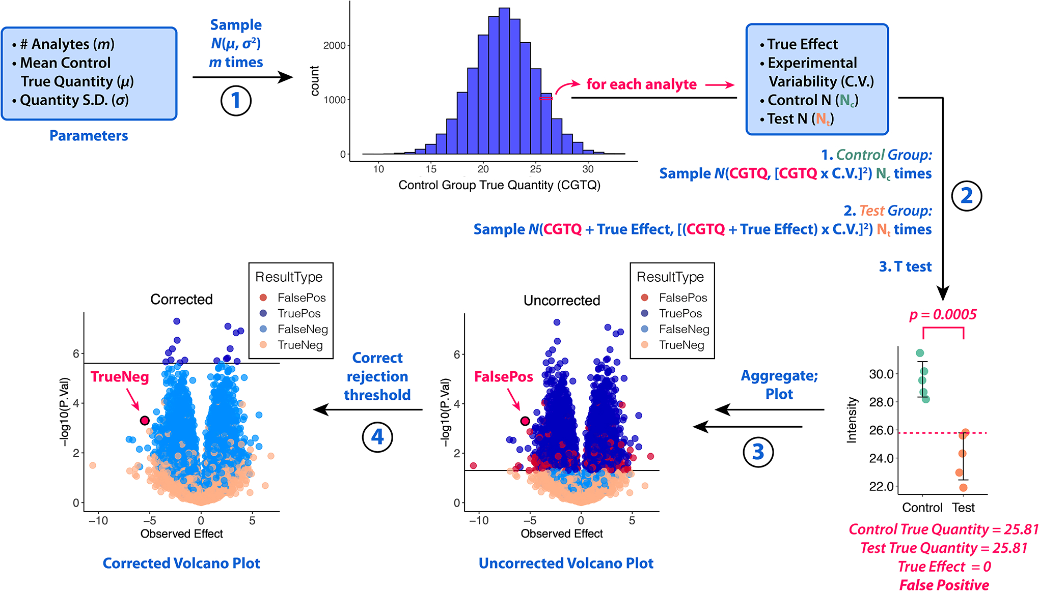
Step 1: The true quantity of each analyte in the control group (CGTQ) is generated. Step 2: Each analyte is “measured” N_c times in the control group and N_t times in the test group. Each analyte has its own True Effect; the Experimental Variability as a coefficient of variation (C.V.) is common among all analytes. A two-sided Welch’s T test is performed for each. Step 3: The results are plotted. Step 4: The p-values or rejection threshold is corrected and the corrected results are plotted. In this example, the Bonferroni method was applied, changing the highlighted analyte from a false positive (FalsePos) to a true negative (TrueNeg). S.D. = standard deviation. N(μ, σ²) represents the normal distribution with mean μ and variance σ².

Second, each analyte is “measured” in N_c control-group samples and N_t test-group samples using a user-specified Experimental Variability as a coefficient of variability (C.V.) and a True Effect. This consists of sampling N(True Quantity, [True Quantity * C.V.]²) N_c times to generate the control group measurements and then N(True Quantity + True Effect, [(True Quantity + True Effect) * C.V.]²) N_t times for the test group. For each analyte, a two-sided T test assuming unequal variances (Welch’s T test) is performed and a p-value is calculated. If the True Effect is nonzero, which is always the case in Model 2 and often the case in Model 3 (see below), Welch’s T test is appropriate. Though Student’s T test could be used where True Effect = 0, effects are nonzero in most real-life studies. Finally, the p-values or rejection threshold is corrected and color-coded volcano plots are generated.

Model 1: All H_0i Are True

First, we simulated quantitative omic experiments in which all H_0i are true: all True Effects were equal to 0 (Figure 2). In this model, there are no underlying differences between the control and test groups. We simulated 500 experiments, each with random values of: m between 100 and 10,000; N_c and N_t between 2 and 10; Experimental Variability (C.V.) between 0.001 and 0.05. The results of a typical simulation of this model are illustrated in Figure 2A. The uncorrected data in Figure 2A contain several false positives. Conversely, p-value correction yields results in which no H_0i are rejected, which is appropriate for a system in which no H_0i are false.

Figure 2. Results of 500 simulations with all H_0i true (all True Effects 0): Model 1.

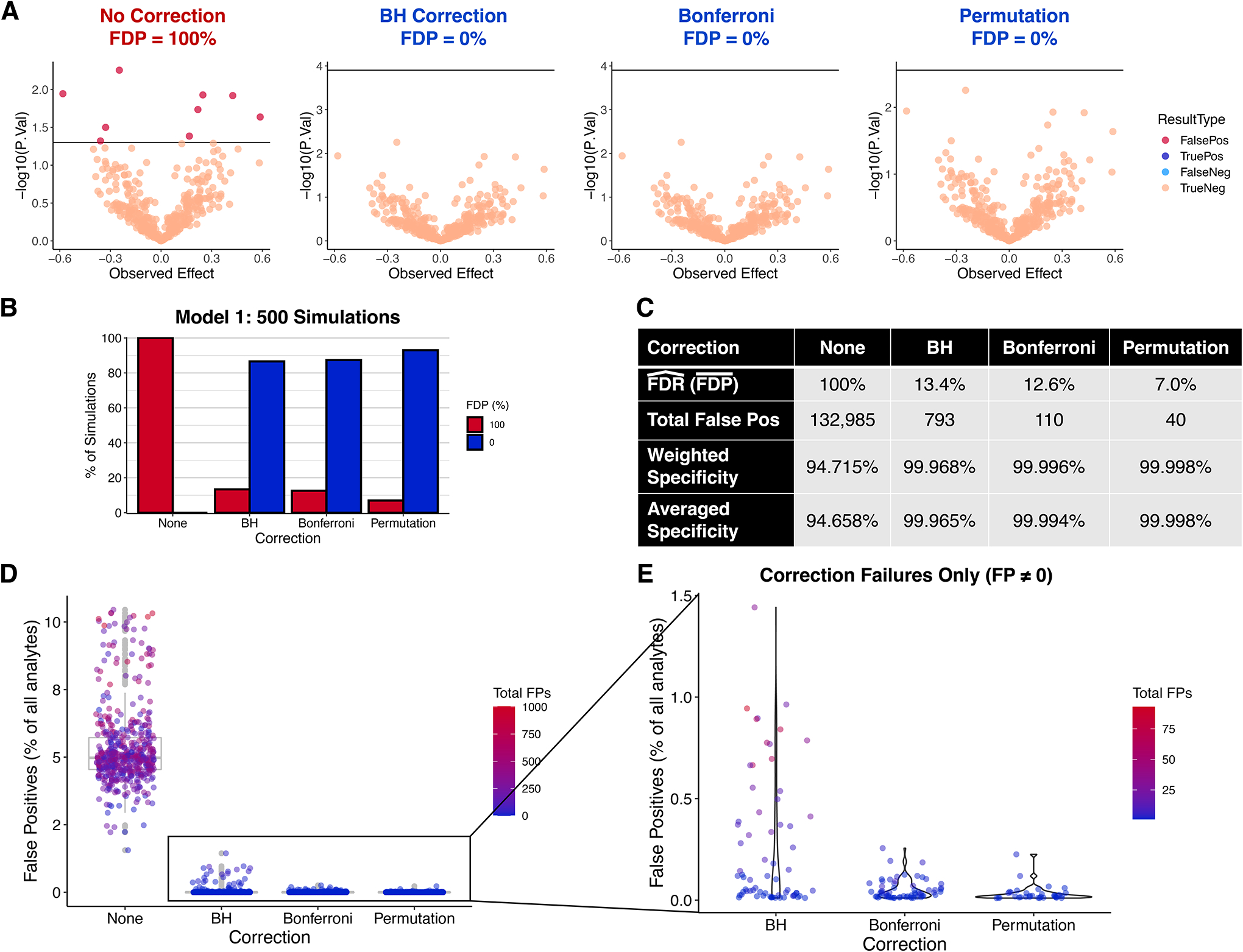
Each simulation had the following randomly generated parameters: m between 100 and 10,000; N_c and N_t between 2 and 10; Experimental Variability (C.V.) between 0.001 and 0.05. A total of 2,516,279 theoretical analytes were measured. A. A typical simulation. Parameters: m = 400, N_c = N_t = 3, Exp. Var. (C.V.) = 0.01. B. Percent of simulations yielding FDP = 100% or 0% under each condition. C. Summary statistics for each condition. Weighted Specificity = (total true neg) / (total true neg + total false pos); Averaged Specificity = mean(observed specificity) = mean[(experiment true negatives) / (experiment true negatives + experiment false positives)]. D. False positives as a percent of analytes. E. Same as D except only corrected data and FP ≠ 0 are included. BH = Benjamini-Hochberg; FDR = false discovery rate (E(FDP)); FDP = false discovery proportion. Hat signifies estimate; bar signifies mean.

Figure 2B–E illustrates the 500 simulations in aggregate. In this model, if there are any statistically significant hits, then FDP = 100%; otherwise, FDP = 0 by definition. Without correction, all simulations yielded an FDP of 100%, whereas correction dramatically reduces the chances of observing false positives (Figure 2B–C). Permutation reduced this probability the most, to 7.0%. Out of over 2.5 million analytes, analysis with correction yielded fewer than 1,000 false hits total (a weighted specificity estimate of >99.9%) whereas over 130,000 hits were falsely identified without correction (Figure 2C).

Doing many simulations enables estimation of the FDR and FWER, the estimates of which, in this model, are equal to each other (see Supplementary Information for proof). While the estimated specificity without correction—94.7%—is close to the expected value of 95%, the estimated FDR for BH is higher than expected (13.4% vs. ≤5%). We also estimate an FWER of 12.6% using Bonferroni which is higher than the expected value of 5%. This appears to be due to imbalanced sample sizes (see below) as well as the artificial lack of any false H_0i. Permutation yielded the best estimated FDR/FWER, with only 40 H_0i rejected out of over 2.5 million (specificity ≈99.998%).

While as many as 10% of the analytes were false positives in uncorrected data, correction always lowered this value to <2% (Figure 2D). Figure 2E illustrates situations in which correction failed to reduce the FDP to 0%. This happened most commonly with BH, and a failure with BH typically resulted in a higher proportional amount of false positives.

Effects of parameters on FDP and specificity with H_0i all true

Without correction, FDP was always 100% and observed specificity was limited to ~95% regardless of Total N (Supplementary Figure S2A). The observed specificity with no correction, BH, and Bonferroni did show some dependence on N, especially when N was close to 12 and either N_c or N_t was low (Low N_x < 4 where Low N_x = min{N_c, N_t}) (Supplementary Figure S2A). This is because observed specificity is proportional to the level of balance between the sample sizes (Supplementary Figure S2B). Raising Total N decreases specificity when one N_x is fixed at a low value, even with BH or Bonferroni (Supplementary Figure S2C–D). With BH, ΔN = 8 yielded an FDP of 100% in every case in these simulations. Permutation-based FDP estimation did not have this problem.

Neither the number of analytes m nor the Experimental Variability (C.V.) had any effect on observed specificity (Supplementary Figure S3). However, a higher m gives a higher total number of false positives: in this study, a single simulation could yield up to 1,000 false hits without p-value correction (Supplementary Figure S3C).

Model 2: All H_0i Are False

Next, we simulated situations in which all genes have a nonzero True Effect, so that all H_0i are false. In this simplistic model, the magnitude of the True Effect is the same for all analytes, where half are positive and the other half are negative. We performed this simulation 3,000 times using the same randomly generated parameters as with Model 1, plus a random True Effect magnitude between 0.01 and 4.

Figure 3A shows an example. Permutation is able to yield a higher observed sensitivity (Obs. Sens.) than no correction. On average, however, sensitivity is reduced with all correction methods (Figure 3B). BH and permutation-based corrections only moderately lowered the average sensitivity from 74.7% to 68.4% and 70.8%, respectively, while Bonferroni yielded 29.2% (Figure 3B). Figure 3C plots the experiment-wise effect of each correction method on observed sensitivity. Whereas BH and Bonferroni always maintain or reduce Obs. Sens., permutation can lower the rejection threshold resulting in an increase in Obs. Sens. (Figure 3A), which occurred in 33.0% of simulations. As Figure 3C shows, permutation was more likely to give an observed sensitivity boost—and the cost of BH correction was reduced—if the uncorrected Obs. Sens. was higher, which can be achieved by increasing N or effect sizes or reducing variability (see below). When uncorrected Obs. Sens. was over 90%, permutation only decreased Obs. Sens. if Low N_x was equal to 3 and ΔN was at least 4 (Supplementary Figure S4A). Because of this boost, permutation yielded an observed sensitivity of 100% more often than without correction: 40.0% of the time, compared to 29.9% for both uncorrected and BH-corrected data and 6.3% for Bonferroni (Supplementary Figure S4B). Permutation was least likely of the three correction methods to reduce Obs. Sens. to 0 (Supplementary Figure S4C).

Figure 3. Results of 3,000 simulations with all H_0i false (all analytes differential): Model 2.

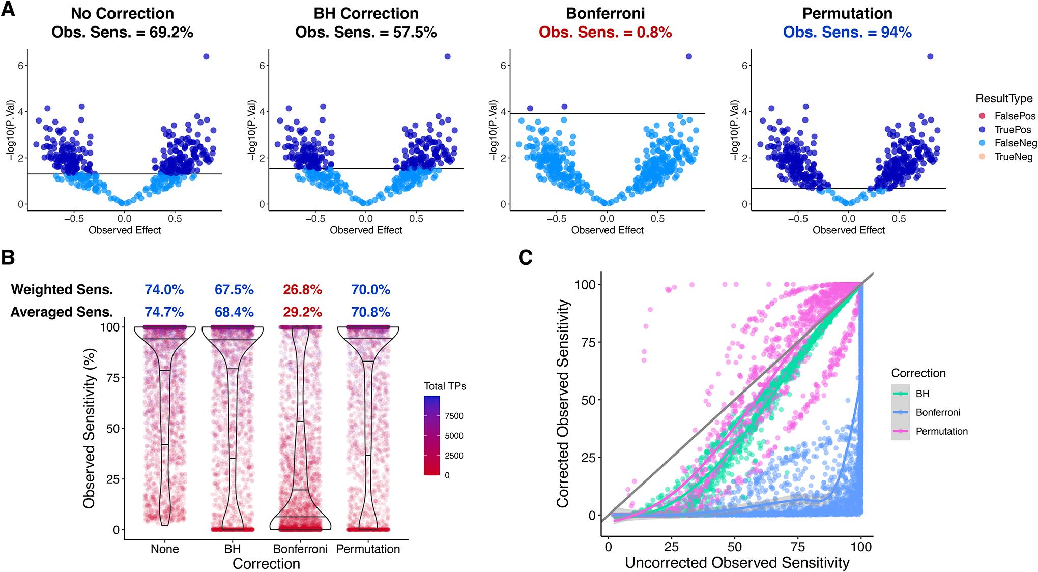
Same random parameter distributions as in 500 Model 1 simulations except True Effect magnitude which was sampled between 0.01 and 4. Given a simulation’s True Effect magnitude (TEm), each analyte was randomly assigned a True Effect of either +TEm or −TEm. A. Example results of a simulation using this model. Parameters: # Analytes = 400; TEm = 0.5; N_c = 4; N_t = 4; Variability (C.V.) = 0.01; Significance Threshold = 0.05. Obs. Sens. = observed sensitivity = (True Positives) / (True Positives + False Negatives). B. Sensitivities from 3,000 simulations. Weighted Sensitivity = Total True Positives / Total Analytes over all simulations. Averaged Sensitivity = mean(Obs. Sens.). C. Observed sensitivity of correction-free analysis vs. observed sensitivity after correction. Diagonal line: y = x. Fit curves generated with LOESS method.

Effects of parameters on sensitivity with H_0i all false

The sensitivity costs of correcting with BH and permutation are modest across a range of parameters in this model, as revealed by Figure 3C but also by the similarities of fit curves when each parameter is plotted against Obs. Sens. (Supplementary Figure S5). Higher N and stronger effects tended to increase sensitivity in all contexts while increased experimental variability decreased sensitivity. We performed multiple linear regression against observed sensitivity with correction method, N_c, N_t, Experimental Variability (C.V.), and True Effect as covariates and used the resulting coefficients to construct a predictor of observed sensitivity (Supplementary Figure S5D). Importantly, even when correcting p-values, it is possible to detect every false H_0i in this model by modifying experimental parameters. Supplementary Figure S6 shows an example in which increasing N was able to completely eliminate the sensitivity cost of p-value correction. Note that increasing Total N from 4 to 20 eliminated the sensitivity cost of permutation-based correction and created a sensitivity benefit.

Model 3: Both True and False H_0i

Neither of these first models are representative of real life, in which both differential and non-differential analytes are usually present. However, simply combining Model 1 with Model 2 results in awkward and unrealistic results when visualized. This problem is true of all models of omic experiments of which we are currently aware.⁸ A normal distribution of True Effects, a realistic alternative, makes it impossible for any H_0i to be true, i.e., for any True Effects to be exactly equal to 0. In order to reconcile nonzero but very small True Effects with the null hypothesis, we found it useful to define a “small” underlying True Effect as less than the biological variability, and then set such “small” True Effects equal to 0 before simulating measurements (Figure 4). To make this possible, biological and technical variabilities were defined separately.

Figure 4. Generation of quantitative omic data with both true and false H_0i: Model 3.

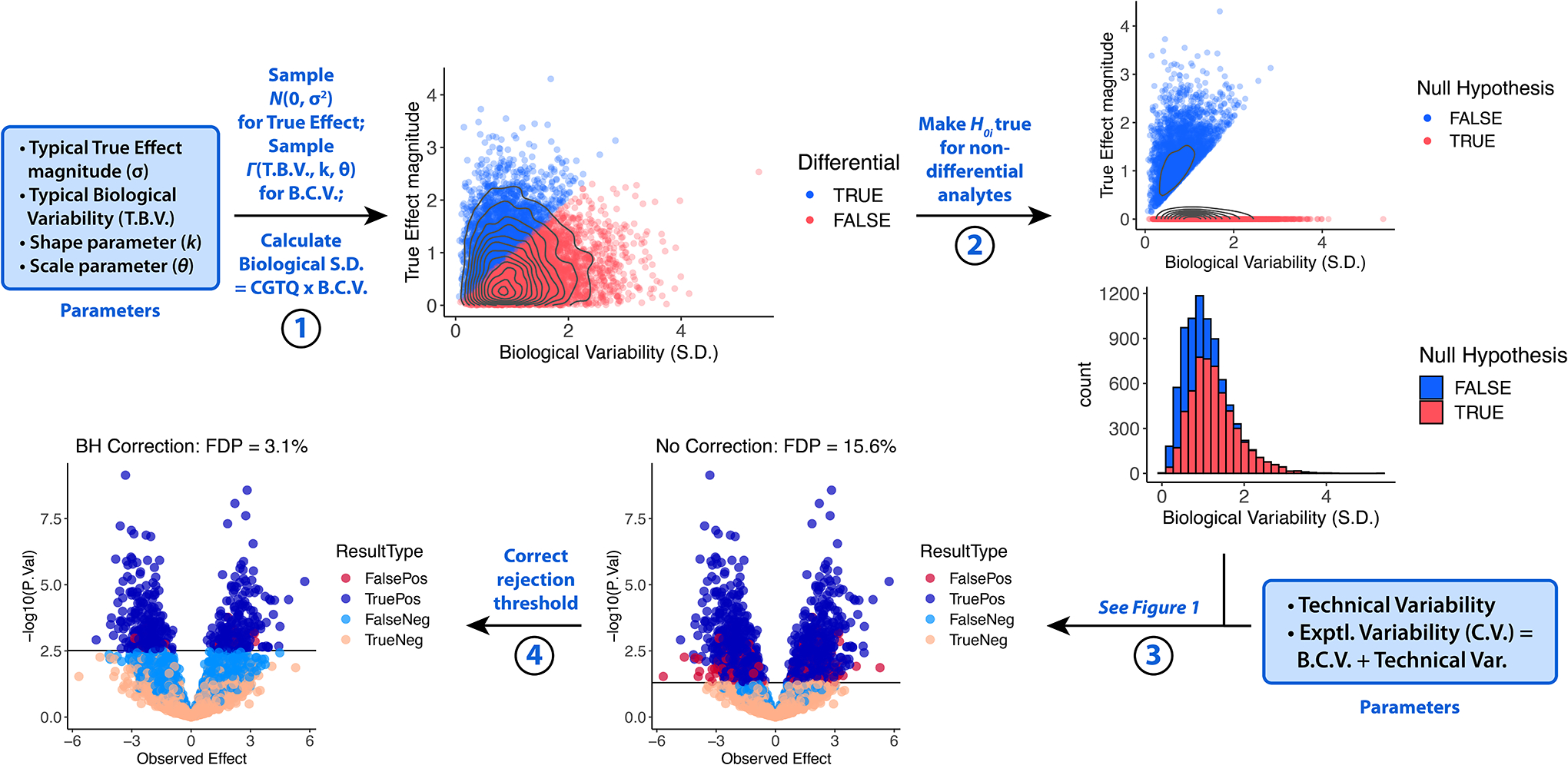
True Effects are generated by sampling a normal distribution m times (Step 1). Biological Variability values (B.C.V.) are sampled from a gamma distribution (Step 1), and for each analyte, if the True Effect magnitude is less than the Biological Variability S.D., then the True Effect is set to equal 0 (Step 2). For each analyte, the Experimental Variability (C.V.) is equal to B.C.V. + Technical Variability, where Technical Variability is an additional chosen parameter (Step 3). Measurements are then simulated and the rejection threshold corrected as illustrated in Figure 1 (Steps 3–4).

First, each analyte in Model 3 was assigned a distinct random Biological Variability (B.C.V.) from a gamma distribution whereas the Technical Variability (C.V.) was the same for all analytes (Figure 4). Each True Effect was sampled from N(0, [Typical Effect magnitude]²). If the True Effect magnitude was less than the Biological Variability S.D. (B.C.V. × Control Group True Quantity CGTQ), H_0i was called true. The True Effects of these “non-differential” analytes were then set to equal 0. Finally, the Technical Variability (C.V.) and B.C.V. were summed to generate the Experimental Variability (C.V.). The resulting sets of Experimental Variabilities and True Effects were used to generate measurements as in Figure 1.

We simulated this model 3,000 times, sampling a random m between 100 and 10,000 and N_c and N_t between 2 and 10 for each simulation. The Typical Effect was sampled between 0.01 and 4. Both Technical Variability (C.V.) and Typical Biological Variability were sampled between 0.001 and 0.05; each analyte’s Biological Variability (B.C.V.) was sampled from a gamma distribution with mean μ equal to Typical Biological Variability, shape parameter 4, and scale parameter 0.5.

An example of this model is shown in Figure 5A, in which all corrections brought the uncorrected FDP of 17.0% below the 5% threshold, with permutation having the highest observed sensitivity among the correction methods (34.2% compared to 29.5% and 4.0% for BH and Bonferroni, respectively).

Figure 5. FDR benefits of p-value correction in 3,000 simulations with both true and false H_0i.

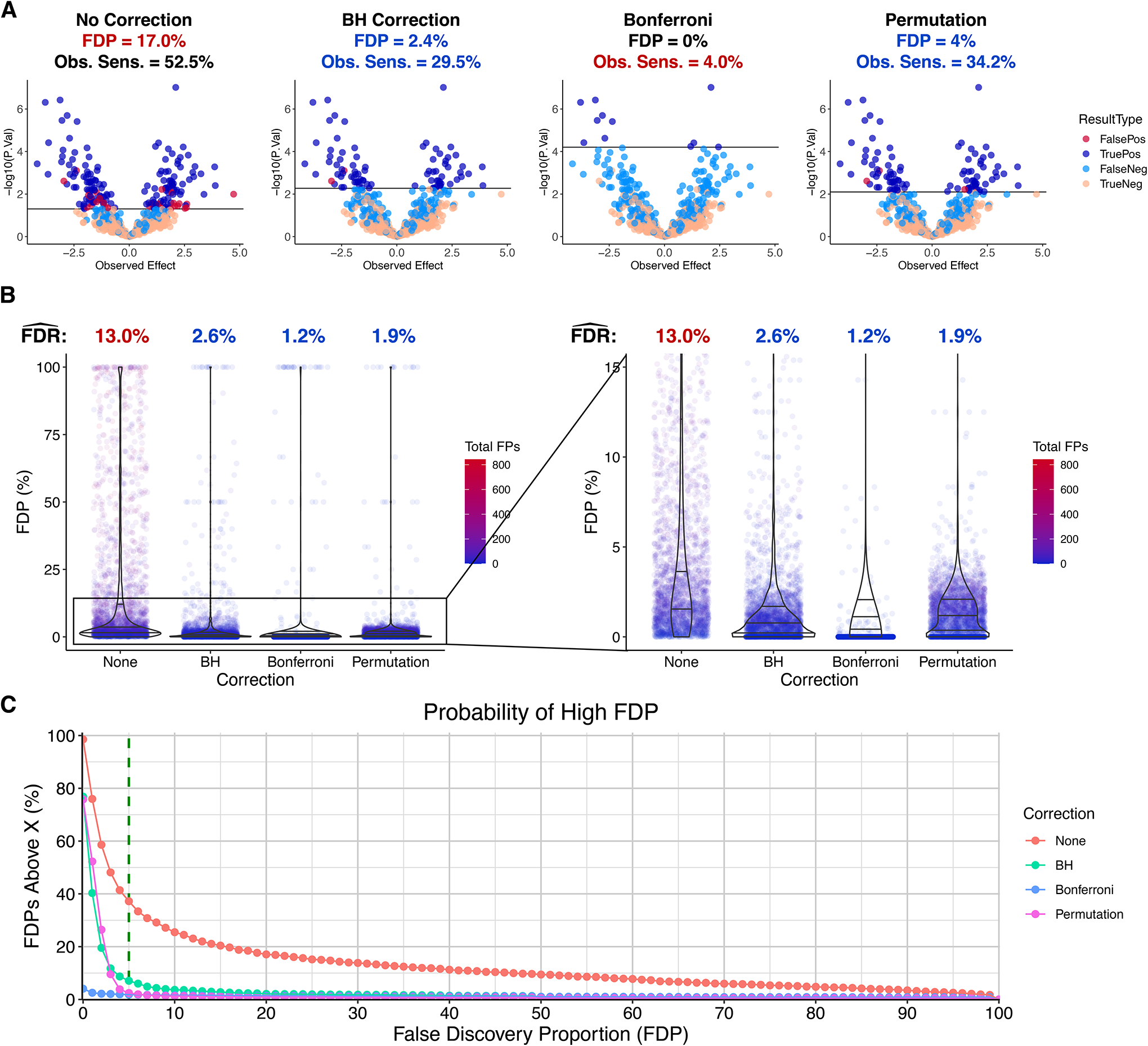
A. Example of Model 3 simulation with both true and false underlying H_0i. Parameters: m = 2,000, N_c = N_t = 11, Typical Biol. Var. (C.V.) = 0.05, Technical Var. (C.V.) = 0.03, Typical Effect = 1, k = 4, θ = 0.5, Significance Threshold = 0.05. B. FDP distributions and FDR estimates. $\widehat{\text{FDR}}=\text{mean}\left(\text{FDP}\right)$. C. For each integer FDP between 0% and 100%, the percent of simulations that yielded an FDP greater than that value (X) is plotted along the Y axis.

FDR benefits of p-value correction with both true and false H_0i

Figure 5B shows that generally lower FDPs were observed when correcting p-values. We also estimated $\text{FDR}=E\left(\text{FDP}\right)\approx \overline{\text{FDP}}$ and found that, as predicted, the FDR was reduced, from 13.0% to 2.6%, 1.2%, and 1.9% by BH, Bonferroni, and permutation, respectively. Importantly, however, no p-value correction method guarantees a low FDP (Figure 5B).

An FDP above 5% is usually an undesirable result. We counted the number of simulations that gave this result and also performed this calculation for every integer percent from 0% to 100% (Figure 5C). Without correction, an FDP over 5% was observed over 35% of the time; there was almost a 1-in-10 chance of getting an FDP over 50%; an FDP over 75% was observed in more than 1 in 20 cases. All three correction methods dramatically reduced the probability of observing a high FDP, but BH was the least effective at avoiding an FDP over 5%: this occurred in 7.1% of cases with BH, 1.8% with Bonferroni, and 2.4% with permutation.

Effects of parameters on FDR and FDP with true and false H_0i

With p-value correction, the effect of Total N and ΔN on FDP was reminiscent of Model 1 (Figure 6A–B, Supplementary Figure S2): Total N had a small and inconsistent effect on FDP with BH and Bonferroni, explained by a deleterious effect of high ΔN; FDP with permutation, meanwhile, was affected by neither N nor ΔN. Increasing Typical Effect improved the FDP with BH and Bonferroni but had no effect with permutation (Figure 6C). Tech. Var. had a minimal effect on FDP, whereas increasing Typical Biological Variability consistently increased FDP in all conditions (Supplementary Figure S7). This is because a high Typical Biological Variability reduces the number and proportional amount of false H_0i and, therefore, hits (Figure 4). Figure 6D–E shows that the presence of a very small number of hits after correction may be interpreted as a warning sign that there may be a high corrected FDP; a high number and proportion of corrected hits tends to indicate a low FDP.

Figure 6. Effects of experimental parameters on FDP with both true and false H_0i.

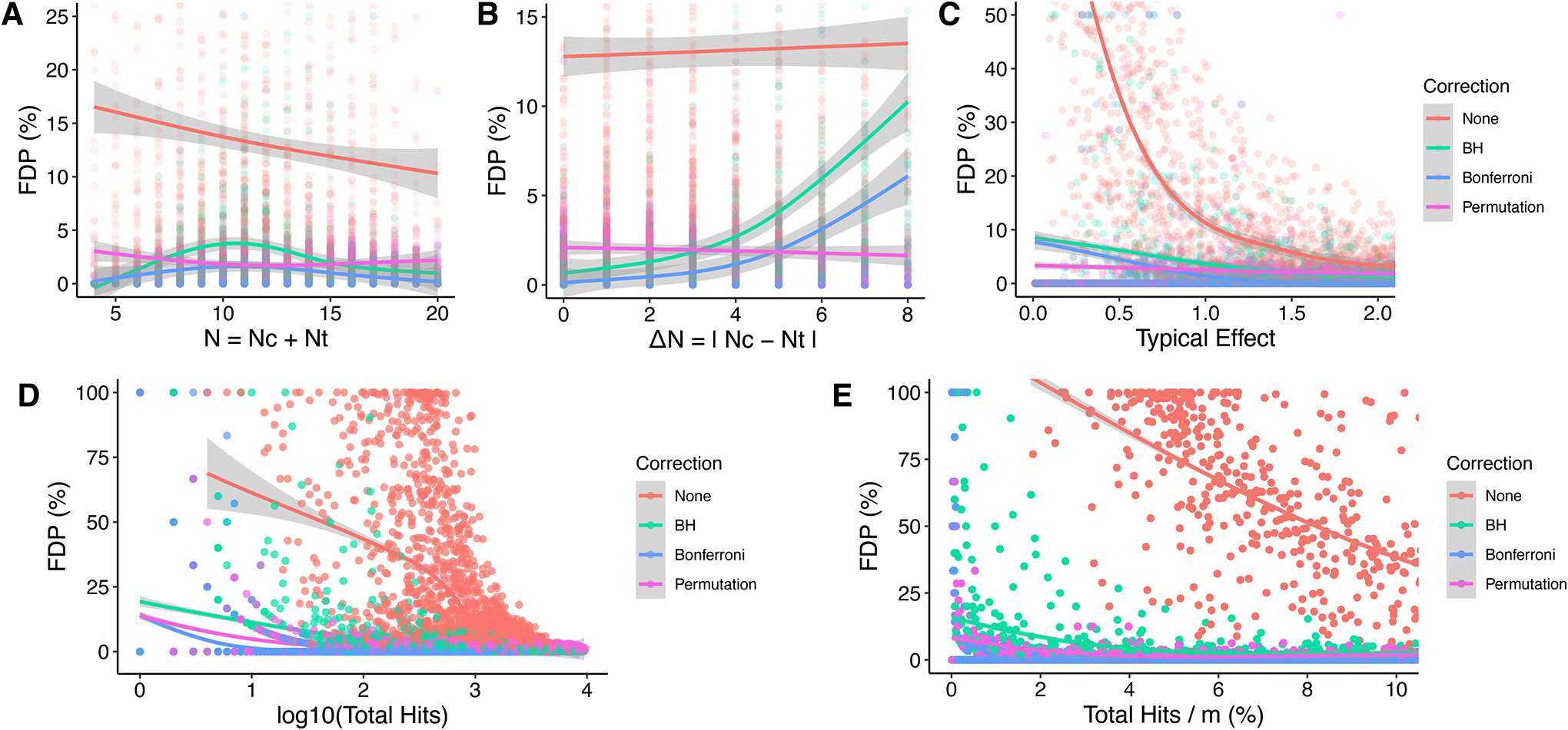
A. Total N vs. FDP. B. ΔN vs. FDP. C. Typical Effect vs. FDP. D. log₁₀(Total Hits) vs. FDP. Total Hits = total H_0i rejected = false positives + true positives. E. (Total Hits / m) * 100% vs. FDP.

Sensitivity costs of p-value correction with true and false H_0i

The effects of correction on sensitivity are shown in Figure 7A–B. The results are similar to those from Model 2, with BH and permutation decreasing sensitivity from 51.0% to 37.6% and 40.3%, respectively, and Bonferroni yielding 10.4% (Figure 7A). Experiment-wise comparisons (Figure 7B) largely recapitulate the results from Model 2 (Figure 3C): Bonferroni causes the greatest loss; losses from BH are modest and with high uncorrected sensitivity are small; permutation causes the smallest loss if any, instead yielding gains in 29.9% of cases.

Figure 7. Sensitivity costs of p-value correction with both true and false H_0i.

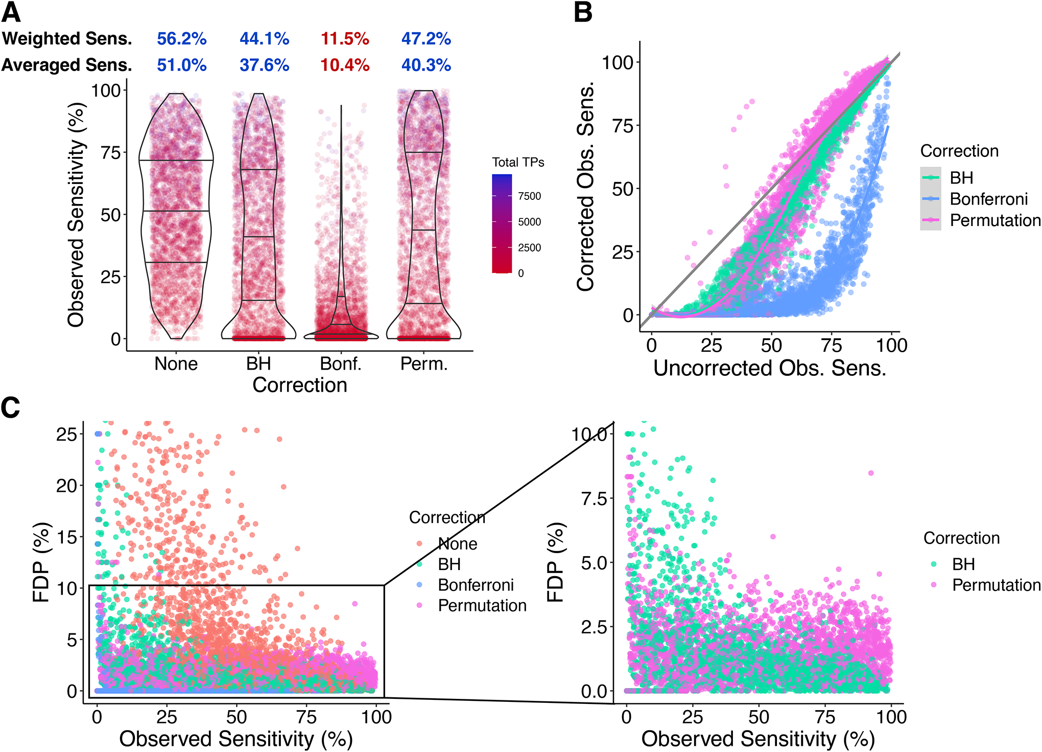
A. Observed Sensitivities and long-run sensitivity estimates. B. Effect of p-value correction on observed sensitivity in each simulation with each method. C. Observed sensitivity vs. FDP.

The relationship between Obs. Sens. and FDP is illustrated in Figure 7C. Because Obs. Sens. is undefined in Model 1 and FDP is always 0 in Model 2, this relationship is only revealed by Model 3. Generally, as experimental parameters give higher Obs. Sens. (high N, low variability, and/or strong effects), the FDP comes down as statistical tests become more accurate. BH and Bonferroni cause the desired decrease in FDP but also a decrease in Obs. Sens. The FDP with permutation is much less dependent on Obs. Sens., covering a relatively flat distribution between 0% and 5%. Thus, permutation offers an improvement over BH in both FDR and sensitivity, which agrees with our observations in Models 1 and 2.

Effects of parameters on sensitivity with both true and false H_0i

As with Model 2, analyses of these simulations show that Total N, ΔN, Technical Variability (Tech. Var.), and Typical Effect can all be modified to reduce the sensitivity cost of p-value correction (Supplementary Figure S8A–D). Typical Biological Variability is also inversely related to Obs. Sens. (Supplementary Figure S8E). A system with a high Typical Effect relative to Typical Biological Variability can be thought of as undergoing strong biological changes; in such systems, the sensitivity cost of correction with BH or permutation is low (Supplementary Figure S8F).

We performed multiple linear regression against Obs. Sens. with Total N, ΔN, Tech. Var., Typical Biological Variability, Typical Effect, and correction method as covariates. A linear combination of Total N, ΔN, and Tech. Var. using the regression coefficients has a strong effect on Obs. Sens., suggesting that good experimental design can greatly reduce the sensitivity costs of correction with BH or permutation even in challenging biological contexts (Supplementary Figure S8G). Including all covariates in a linear combination, even the sensitivity cost of Bonferroni correction can be erased (Supplementary Figure S8H). With permutation, Obs. Sens. was reduced by a Low N_x equal to 3 with imbalanced sample sizes as observed in Model 2 (Supplementary Figure S8I). In summary, the sensitivity costs of correction can be minimized by balancing sample sizes, increasing sample sizes (especially having a Low N_x of at least 4), minimizing variability, and maximizing effect sizes.

Supplementary Figure S9 gives an example of how increasing Total N can eliminate the sensitivity cost of correction. Clearly, N_c = N_t = 3 is not suitable for this system, as the uncorrected data have FDP = 37.5% and no differential analytes are detected with correction. Increasing Total N to 40, observed sensitivities with correction increase dramatically, though Bonferroni still misses many false H_0i. An increase to 500 allows perfect detection of false H_0i with all three methods (100% Obs. Sens.). Importantly, even at this extremely high N, the FDP of uncorrected data is still >5%: 7.2% of hits are false.

As an example of the costs and benefits of p-value correction in real-life data, we analyzed publicly available measurements of a yeast-human digest mixture in which none of the human peptides are differential and all of the yeast peptides are (Supplementary Figure S10).¹² In agreement with our simulations, correction reduced FDP from 24% to <6%. Bonferroni had an observed sensitivity of 0.5% while BH and permutation yielded 37% and 64% respectively.

Discussion

In existing models of quantitative omic experiments, either the data are not visualizable by volcano plot because fold changes are never calculated⁸ or the data do not resemble real life because measurements of non-differential and differential analytes are sampled from distributions that are too different from each other.⁵ Other models fail to address the very small effect magnitudes of differential analytes whose effect sizes are sampled from continuous distributions.⁶ We addressed these issues with Model 3, generating data that contain both true and false H_0i and resemble real-life data when visualized by volcano plot. In SIMPLYCORRECT we have a tool that allows users to explore parameters beyond the ranges discussed here, and we provide the R code for readers to adapt to their own interests.

Although permutation-based FDP estimation is used by many mass spectrometrists via the Perseus platform¹³ or the SAMR package¹⁰, performing a simple permutation-based threshold correction in a single line of code, as one can do with BH and Bonferroni, has not been possible. We optimized an implementation of permutation-based FDP estimation with Rcpp^14,15,16 and Boost C++ Headers for R¹⁷ and made it available via an open-source R package (https://github.com/steven-shuken/permFDP), making it now easy to perform permutation-based correction with a single line of code.

Assumptions in our models include the independence of random variables, distribution shapes, and the commonality of distributions across analytes. Our use of the normal distribution was based on log-transformed mass-spectrometric intensities which are generally assumed to be normally distributed, but RNA sequencing data are better modeled by a negative binomial distribution and tested using Wald or likelihood ratio tests.¹⁸ Non-parametric testing is also an area for further exploration. Biological variabilities are largely unknown, but considering biological variability as a distinct parameter is valid in many situations, e.g., choosing a species when studying Alzheimer’s disease.¹⁹ In some contexts, increasing the effect size may also be possible, e.g., using a model or treatment that perturbs the system more strongly than another.²⁰ Future experimental work may be useful in characterizing yet-unknown ome-wide distributions of variabilities and effects, e.g., using experimental designs that allow separate characterization of biological variabilities and technical variabilities.²¹

Independence may be our strongest assumption since biological omic data are often correlated.¹¹ However, Models 1 and 2 can describe situations in which test statistics only vary because of technical variability, which is likely to be independent in a real-life proteomic or transcriptomic study. In Model 3, this is not the case. Dependence is known to affect the abilities of correction methods to control the FDR; dependence-derived error with different correction methods are an active area of study.^22,8 Future work will examine correlated biological variation as well as cutting-edge correction methods, such as the usage of knockoff variables,²³ that are designed to control the FDR effectively in correlated data.

Despite these shortcomings, we were able to reach several reasonable conclusions and insights. A set of uncorrected p-values can resemble one with many true hits and yet still be comprised entirely of false positives. We therefore believe that the sensitivity costs of p-value correction must always be sustained in order to control the FDR, except perhaps in the case of unpublished explorations that are immediately validated.

We found that correction with BH or permutation generally eliminates a modest number of true hits unless the experimental design is weak. Indeed, all three methods investigated here are capable of retaining all true hits with high enough N or low enough variability. Permutation-based FDP estimation can reveal additional true hits beyond those in the uncorrected data. Permutation reliably outperforms BH; though high ΔN and Low N_x = 3 reduce sensitivity with permutation, these conditions elevate FDR with BH (Figure 6B).

Most parameters affect sensitivity predictably: high N, low variability, and strong effects yield a high sensitivity while correcting p-values. FDR is not very sensitive to experimental parameters with correction, generally remaining low. However, our studies reveal an apparently not-well-known importance of balancing sample sizes, which improves FDR and/or sensitivity depending on correction method.

Finally, we took advantage of publicly available experimental data in which both differential and non-differential analytes are present. Trends observed in simulations were also observed in this example: reduction of the FDP from an unacceptable level to a tolerable one; the superior sensitivity of permutation-based correction; and increased effect size yielding a reduction in sensitivity cost (Supplementary Figure S10).

Though the appropriate course of action depends on the individual experiment, we present the following guidelines for design of a quantitative omic experiment: (1) Choose a system with low variability and strong effects. (2) Balance the sample sizes, i.e., N_t = N_c, and use N_x ≥ 4. (3) Minimize technical variability. (4) Correct p-values using permutation-based FDP estimation. (5) If there are very few statistically significant hits after correction (<10 or <1% of all analytes), validate them.

References

- 1.Baker M Reproducibility crisis: Blame it on the antibodies. Nature 2015, 521, 274–276. [DOI] [PubMed] [Google Scholar]
- 2.Perng W; Aslibekyan S Find the Needle in the Haystack, Then Find It Again: Replication and Validation in the ‘Omics Era. Metabolites 2020, 10, 286. [DOI] [PMC free article] [PubMed] [Google Scholar]
- 3.Johnson ECB; Dammer EB; Duong DM; Ping L; Zhou M; Yin L; et al. Large-scale proteomic analysis of Alzheimer’s disease brain and cerebrospinal fluid reveals early changes in energy metabolism associated with microglia and astrocyte activation. Nature Med. 2020, 26, 769–780. [DOI] [PMC free article] [PubMed] [Google Scholar]
- 4.Rice JA Fishing Expeditions. In: Mathematical Statistics and Data Analysis. Third ed. Delhi: Cengage Learning India Private Limited; 2007. p. 458. [Google Scholar]
- 5.Brinster R; Köttgen A; Tayo BO; Schumacher M; Sekula P Control procedures and estimators of the false discovery rate and their application in low-dimensional settings: an empirical investigation. BMC Bioinformatics 2018,19, 78. [DOI] [PMC free article] [PubMed] [Google Scholar]
- 6.Korthauer K; Kimes PK; Duvallet C; Reyes A; Subramanian A; Teng M A practical guide to methods controlling false discoveries in computational biology. Genome Biol. 2019, 20, 118. [DOI] [PMC free article] [PubMed] [Google Scholar]
- 7.Head ML; Holman L; Lanfear R; Kahn AT; Jennions MD The Extent and Consequences of P-Hacking in Science. PLoS Biol. 2015, 13, e1002106. [DOI] [PMC free article] [PubMed] [Google Scholar]
- 8.Kluger DM; Owen AB A central limit theorem for the Benjamini-Hochberg false discovery proportion under a factor model. arXiv.org 2021, URL: https://arxiv.org/abs/2104.08687. Accessed November 9, 2022. [Google Scholar]
- 9.Benjamini Y; Hochberg Y Controlling the False Discovery Rate: a Practical and Powerful Approach to Multiple Testing. J. R. Statist Soc B 1995, 57, 289–300. [Google Scholar]
- 10.Tusher VG; Tibshirani R; Chu G Significance analysis of microarrays applied to the ionizing radiation response. Proc. Natl. Acad. Sci 2001, 98, 5116–5121. [DOI] [PMC free article] [PubMed] [Google Scholar]
- 11.Shuken SR; Rutledge J; Iram T; Losada PM; Wilson EN; Andreasson KI; Leib RD; Wyss-Coray T Limited proteolysis-mass spectrometry reveals aging-associated changes in cerebrospinal fluid protein abundances and structures. Nature Aging 2022, 2, 379–388. [DOI] [PMC free article] [PubMed] [Google Scholar]
- 12.Schweppe DK; et al. “Characterization and Optimization of Multiplexed Quantitative Analyses Using High-Field Asymmetric-Waveform Ion Mobility Mass Spectrometry.” Anal. Chem 2019, 91, 4010–4016. [DOI] [PMC free article] [PubMed] [Google Scholar]
- 13.Tyanova S; Temu T; Sinitcyn P; Carlson A; Hein MY; Geiger T; et al. The Perseus computational platform for comprehensive analysis of (prote)omics data. Nature Methods 2016, 13, 731–740. [DOI] [PubMed] [Google Scholar]
- 14.Eddelbuettel D; Francois R Rcpp: Seamless R and C++ Integration. J. Statistical Software 2011, 40, 1–18. [Google Scholar]
- 15.Eddelbuettel D Seamless R and C++ Integration with Rcpp. Springer. New York: ISBN 978-1-4614-6867-7. [Google Scholar]
- 16.Eddelbuettel D; Balamuta JJ Extending R with C++: A Brief Introduction to Rcpp. The American Satistician 2018, 72. [Google Scholar]
- 17.Eddelbuettel D; Emerson JW; Kane MJ BH: Boost C++ Header Files. R package version 1.78.0–0; URL: https://CRAN.R-project.org/package=BH. Accessed November 9, 2022. [Google Scholar]
- 18.Love Michael I.; Huber W; Anders S “Moderated estimation of fold change and dispersion for RNA-seq data with DESeq2.” Genome Biol. 2014, 15, 550. [DOI] [PMC free article] [PubMed] [Google Scholar]
- 19.Tuttle AH; Philip VM; Chesler EJ; Mogil JS Comparing phenotypic variation between inbred and outbred mice. Nature Methods 2018, 15, 994–996. [DOI] [PMC free article] [PubMed] [Google Scholar]
- 20.Elder GA; Sosa MAG; De Gasperi R Transgenic Mouse Models of Alzheimer’s Disease. Mount Sinai J. Med 2010, 77, 69–81. [DOI] [PMC free article] [PubMed] [Google Scholar]
- 21.Robasky K; Lewis NE; Church GM “The role of replicates for error mitigation in next-generation sequencing.” Nature Rev. Genetics 2014, 15, 57–62. [DOI] [PMC free article] [PubMed] [Google Scholar]
- 22.Fithian W; Lei L Conditional calibration for false discovery rate control under dependence. arXiv.org. 2020, URL: https://arxiv.org/abs/2007.10438. Accessed November 9, 2022. [Google Scholar]
- 23.Candès E; Fan Y; Janson L; Lv J Panning for gold: ‘model-X’ knockoffs for high dimensional controlled variable selection. J. R. Statist. Soc B 2018, 80, 551–577. [Google Scholar]
Associated Data
This section collects any data citations, data availability statements, or supplementary materials included in this article.