Abstract
Ultrasound computed tomography (USCT) is an emerging technology that offers a noninvasive and radiation-free imaging approach with high sensitivity, making it promising for the early detection and diagnosis of breast cancer. The speed-of-sound (SOS) parameter plays a crucial role in distinguishing between benign masses and breast cancer. However, traditional SOS reconstruction methods face challenges in achieving a balance between resolution and computational efficiency, which hinders their clinical applications due to high computational complexity and long reconstruction times. In this paper, we propose a novel and efficient approach for direct SOS image reconstruction based on an improved conditional generative adversarial network. The generator directly reconstructs SOS images from time-of-flight information, eliminating the need for intermediate steps. Residual spatial-channel attention blocks are integrated into the generator to adaptively determine the relevance of arrival time from the transducer pair corresponding to each pixel in the SOS image. An ablation study verified the effectiveness of this module. Qualitative and quantitative evaluation results on breast phantom datasets demonstrate that this method is capable of rapidly reconstructing high-quality SOS images, achieving better generation results and image quality. Therefore, we believe that the proposed algorithm represents a new direction in the research area of USCT SOS reconstruction.
Keywords: Ultrasound computed tomography, Image reconstruction, Deep learning, Speed-of-sound, Breast imaging
Introduction
Breast cancer is the most prevalent cancer among women, and its incidence has been increasing in recent years [1]. Early detection is crucial for a favorable prognosis [2]. However, the most commonly used mammography can be limited by dense breast tissue, leading to missed and inaccurate diagnoses [3]. Ultrasound computed tomography (USCT), especially transmission tomography, has shown great potential in detecting breast cancer due to its ability to obtain quantitative acoustic parameters such as the speed-of-sound (SOS) and attenuation [4, 5]. Tumor tissues typically have higher SOS values than normal tissues [6], making quantitative reconstructed SOS images an effective tool to assist in breast tumor diagnosis.
SOS reconstruction is a challenging nonlinear inverse problem. Some methods rely on simplified approximations. One such approach is travel-time tomography based on the straight or bent-ray approximation, which neglects diffraction effects and has a fast speed but low spatial resolution [7]. Another approach is based on Born or Rytov approximations to linearize the forward scattering problem, which provides relatively higher resolution but may not be suitable for imaging breasts with large SOS contrasts [8]. Full-waveform inversion (FWI) accurately models the physics of wave propagation and has the highest reconstruction accuracy, but it requires high computational costs [9].
To improve reconstruction efficiency, researchers have employed deep learning methods to directly reconstruct SOS images from the signal domain, achieving remarkable success [10–19]. One possible method is model-driven deep learning methods, which incorporate networks into unrolling iterative reconstruction algorithms [10–13]. Vishnevskiy et al. introduced a variational network for pulse-echo SOS estimation under limited view by unfolding a model-based reconstruction method [10–12]. The variational network employs the adjoint of projection operators to learn the gradient of the regularizer from data, eliminating the need for manual regularization tuning. Fan et al. proposed a model-data-driven method by unrolling the primal-dual algorithm based on the paraxial approximation of the Helmholtz equation, using U-Net [20] to replace the forward adjoint operator [21]. However, the paraxial approximation is only applicable when the angle between the direction of propagation and the z-axis is small. These methods still involve an iterative process, which is time-consuming and computationally expensive and thus not suitable for real-time imaging in clinical applications.
Pure data-driven deep learning reconstruction has also achieved success in image reconstruction tasks due to its ability to automatically learn feature representations from large datasets and perform highly nonlinear mappings [15–19, 22]. However, methods such as AUTOMAP [22] that utilize several stacked fully connected layers may suffer from overfitting and require large memory capacities for larger image sizes. To address this issue, researchers have turned to fully convolutional neural networks [15–19], most of which are based on the U-Net structure [20]. Some networks [15–18] use frequency domain pressure data as input, which may lack flexibility for various array configurations. Other networks, such as DeepUCT [22] take the entire time-series data as input, leading to significantly increased computational costs, especially when dealing with a large number of transducers. In contrast, employing time-of-flight (TOF) as input can address these issues, enabling more flexible and efficient reconstruction.
Furthermore, it should be noted that SOS reconstruction in USCT is a nonlinear inverse problem that can be solved with generative models, such as generative adversarial networks (GANs) [23]. One notable GAN variant is WGAN-GP [24, 25], which incorporates the Wasserstein distance and the gradient penalty as the discriminator loss, avoiding model collapse and gradient disappearance in original GANs. However, it lacks control over the generated outputs. In contrast, Pix2Pix [26], a conditional GAN-based approach [27], provides enhanced control by utilizing conditional inputs for the generator. It enables domain transformations by minimizing pixel reconstruction error and adversarial loss. Additionally, the discriminator network incorporates correlation between the input and generated images, facilitating more effective discrimination.
Building upon these concepts, a novel approach called Direct SOS reconstruction with Spatial-Channel Attention Wasserstein GAN (DSA-GAN) is proposed to associate TOF information with the SOS distribution without relying on any physical prior. The DSA-GAN takes the arrival time distribution as input and directly generates SOS images through the generator. The discriminator is employed to evaluate the discrepancy between the generated and real SOS images, using it as a regularization term to guide the optimization of the generator. Moreover, a perceptual loss is added to the loss function to help the network better learn advanced semantic information in the SOS distribution. Qualitative and quantitative experimental results demonstrate that DSA-GAN can achieve rapid and high-quality reconstruction of SOS images for healthy breasts at different density levels and breasts with lesions.
Methods
Problem formulation
In USCT imaging, a commonly employed configuration is a ring transducer array composed of M uniformly distributed transducers, as shown in Fig. 1a. In this imaging setup, each individual transducer element emits a spherical wave that propagates inside the array, interacting with objects present in the medium. Subsequently, all transducer elements act as receivers to record the raw data. The imaging process involves sequentially emitting waves from each element while recording the received wave signals for inverse imaging.
Fig. 1.
a Schematic illustration of SOS imaging using a ring transducer array in USCT. b A schematic of the Radon transform in the straight-ray assumption, where r represents the position of the individual detector element, and denotes the angular along the transmitter-emitter direction
In FWI, the main objective is to optimize the model parameters to minimize the discrepancies between the observed time series and the numerically generated modeled data , which can be formulated as:
| 1 |
where is the unknown model parameter vector related to SOS, acoustic density, and attenuation. The operator describes how to compute the data from the model parameters, which is implemented as the acoustic wave equation. It is worth noting that the wave equation introduces a nonlinear relationship between pressure and model parameters, making the optimization problem inherently nonlinear as well.
Alternatively, travel-time tomography employs a high-frequency approximation to the acoustic wave equation, assuming that the physical energy propagates along ray paths. The TOF between an emitter and a receiver can be calculated by integrating the slowness (i.e., reciprocal of the SOS) along the acoustic propagation path. The imaging region is discretized into grids. The goal of the inverse problem is to find a slowness distribution that can well describe the observed travel times , i.e.,
| 2 |
where denotes the ray-length matrix, which depends on the current SOS distribution, leading to a nonlinear relationship between and .
Therefore, both travel-time tomography and FWI pose nonlinear problems that require iterative optimization processes and have high computational requirements. In the proposed method, the conventional optimization procedures are substituted with a neural network training process, which presents a promising alternative.
The network is designed from TOF data, which aligns with travel-time tomography. Under the straight-ray assumption, which is based on the Radon transform, the Radon projections corresponding to a certain position in the spatial domain form a sinusoid in the sinogram data, as depicted in Fig. 1b. However, when the bent-ray assumption is introduced, this relationship becomes more intricate. The projection of a point may involve multiple elements, including the sinusoidal curve and its expansion areas. To determine the ray path that best approximates the observed travel time, iterative processes involving forward and inverse computations are employed. To overcome this limitation, one can explore the application of attention modules to adaptively learn the relationships between specific positions in the TOF image, enabling a more precise determination of relevant features during the reconstruction process.
Framework based on conditional Wasserstein GAN
Figure 2 illustrates our proposed network architecture, which draws inspiration from WGAN-GP [24, 25] and the successful Pix2Pix framework [26] designed for image-to-image translation. Within this framework, a generator G is utilized to directly map the TOF domain to the image domain, generating synthetic SOS images, while a discriminator D distinguishes between real and synthetic SOS images. The generator aims to generate results that closely resemble the real SOS image to deceive the discriminator, which in turn is trained to be more discerning and accurately identify the generated SOS images. The generator and discriminator are trained iteratively, competing against each other to enhance the overall generative performance.
Fig. 2.
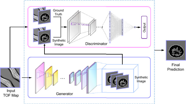
A schematic diagram of the overall structure of the DSA-GAN
Loss function
In the image-to-image USCT SOS image reconstruction task, the loss functions of the discriminator and generator are minimized as follows:
| 3 |
| 4 |
where represents the TOF information extracted from the transmission signals with random noise and serves as the input to the generator, acting as the conditional information. is the SOS image generated from the generator, i.e., , which comes from the generated sample distribution . is the ground truth SOS image, which comes from the real sample distribution . represents a random sample between and , that is, , where is a random variable that follows a uniform distribution (i.e., ). The first two terms in Eq. (3) represent the Wasserstein distance, and the last term represents the gradient constraint. is a constant weight parameter that biases the gradient of the differentiable discriminator towards 1, and denotes the gradient of the discriminator.
Furthermore, the L1 loss and perceptual loss are introduced to ensure the similarity between the generated images and the target images:
| 5 |
| 6 |
where denotes the VGG-19 feature extractor [28] and n and d represent the number of pixels and feature maps in each feature map, respectively. The term corresponds to the features of the ground truth, while represents the features of the generated SOS image.
The final loss function of the generator can be represented as:
| 7 |
where and are weight parameters that balance the contributions of perceptual loss, content loss, and adversarial loss.
Network architecture
Generator
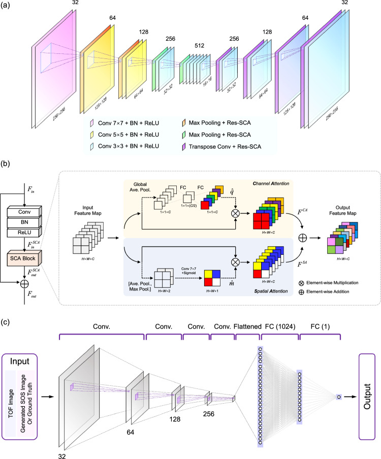
The generator of DSA-GAN employed a classical encoder-decoder structure [29], as depicted in Fig. 3a, as the input and output belong to different domains and low-level information sharing is unnecessary for this image-to-image domain transformation task. Therefore, unlike in Pix2Pix, a U-Net with skip-connection structures is not needed. The encoder converts the high-dimensional TOF map into an embedded representation, while the decoder generates the high-dimensional SOS image. In the encoder, the filter size of the convolutional layers gradually decreases. The first two layers have a size of , followed by five layers with a size of , and the remaining layers have a size of . By utilizing a larger filter size in the initial layer, the network can capture a broader range of information by covering a larger neighborhood region of the input TOF map. This is crucial since a single pixel in the reconstructed image corresponds to scattered areas in the TOF map. To maintain the sparsity of high-dimensional feature representations, the number of convolutional filters in the encoder increases, and correspondingly, the number of channels in the feature maps is doubled, with sizes of 32, 64, 128, 256, and 512. The input and output sizes of the generator are both fixed at pixels.
Fig. 3.
The architecture of the a generator, b residual spatial-channel attention module (Res-SCA), and c discriminator in DSA-GAN
Furthermore, a Residual Spatial-Channel Attention module (Res-SCA) is incorporated after each down (up) sampling, as shown in Fig. 3b. This module integrates channel attention (CA) [30] and spatial attention (SA) [31] with the conventional residual block to enhance useful features. Suppose that the input to the SCA module is denoted by , and it consists of C feature maps with each map having a size of . can be expressed as in CA, where is the c-th feature map and in SA, where denotes the feature in the (i, j) position.
CA module The global average pooling is applied to shrink the spatial dimensions of the input feature map , obtaining the channel-wise statistics . The set of these descriptors is then processed by two fully connected layers to compute scaling factors for each input channel. The first layer, which is parameterized by the weight set , performs channel downscaling by reducing the number of channels in the input signal by a factor of . The resulting low-dimensional signal is then passed through the second layer, which is parameterized by the weight set , to perform channel-upscaling and restore the original number of channels. As a result, the channel-wise rescaling weights are:
| 8 |
where and are the ReLU and sigmoid activation functions, respectively. The channel scaling factors are then applied to reweight the input channels through elementwise multiplication with the input feature map, as shown below:
| 9 |
SA module The input feature undergoes average pooling and maximum pooling along the channel dimension, resulting in two channel feature maps, and , respectively. These feature maps are then concatenated along the channel dimension, forming the concatenated feature map . Next, a convolutional filter with weight is applied to the concatenated feature map , compressing it along the channel dimension. After the convolutional layer, the sigmoid activation function is applied to obtain the weight coefficients :
| 10 |
The new feature map is then obtained by elementwise multiplication of and the input feature map :
| 11 |
Finally, the output of the CA and SA modules are added to the original input feature map using a residual skip connection, generating the final output of the Res-SCA module.
Discriminator
The discriminator in this study is based on the design principles of WGAN and Pix2Pix, as depicted in Fig. 3c. The network takes as input both the predicted SOS images from the generator (or ground truth) and the original input TOF images as conditions, which ensures that the generator produces results that are consistent with the content of the original images. However, the PatchGAN design used in Pix2Pix is not suitable for this study, as it assumes that different image regions are independent of each other, whereas in this case, there is no one-to-one correspondence between the input and output pixels. In this study, each pixel in the arrival time distribution image has physical significance in terms of its horizontal and vertical coordinates and is associated with the complete SOS image, so the discriminator needs to operate on the entire space. The convolutional layers have a filter size of and numbers of 32, 32, 64, 64, 128, 128, 256 and 256. Two fully connected layers with 1024 and 1 neurons follow these convolutional layers. A Leaky ReLU activation layer [32] follows each convolutional layer and the first fully connected layer. The odd-indexed convolutional layers have a step size of 1, while the even-indexed layers have a step size of 2 to reduce the image scale. The sigmoid function layer of the last fully connected layer of the original GAN’s discriminator is removed, and the Wasserstein distance is used to measure the difference between the generated and real images.
Implementation details
During training, the generator and discriminator were trained alternately. In each iteration, the discriminator was trained 5 times before the generator was trained once. The filter weights of each layer were initialized by random values drawn from a Gaussian distribution with zero mean and standard deviation of 0.01. The leaky ReLU layer of the discriminator used a slope of 0.2 for negative inputs. The channel reduction rate in the Res-SCA module was set to 2. The SGD optimizer was utilized with a learning rate of , and the batch size was set to 16. In the loss function, the weight parameters for the pixel loss and perceptual loss were 0.1 and 0.01, respectively. The weight parameter for the gradient penalty term was set to 10. The network was implemented in Python 3.7 using TensorFlow as the framework and was trained on a server with four NVIDIA GeForce RTX 2080Ti GPUs, each with 11 GB of memory.
The proposed method was evaluated against commonly used traditional methods starting from TOFs, including FBP [33] and the bent-ray method with Laplacian regularization (referred to as Laplacian) [7]. FBP is based on straight-ray assumptions, while Laplacian incorporates bent-ray assumptions from travel-time tomography. Additionally, a comparison was made with DSA-Net, which shares the same structure as the generator network. DSA-Net can be considered a representative of studies employing an architecture based on the U-Net structure [15–19]. The training of DSA-Net employed the SGD optimizer with a gradually decreasing learning rate ranging from to . All the compared methods utilized the best parameter settings for evaluation.
Results
Synthetic circle dataset
This dataset consists of images containing randomly generated nonoverlapping uniform disks, each with a constant density and SOS value, without considering acoustic attenuation. These disks represent neighboring soft tissues, with SOS values ranging from 1450 to 1583 m/s. They are set against a background of water with an SOS value of 1480 m/s. The images were obtained using a 256-element transducer ring array that was uniformly distributed and had a diameter of 160 mm. To emulate the errors that can occur during travel time selection, the simulated TOF map obtained using the Eikonal solver was modified with Gaussian random noise, with a standard deviation of 10 ns. The dataset consists of 60,000 pairs, with 48,000 pairs used for training and 12,000 pairs reserved for testing.
The accuracy of the reconstruction was assessed using three widely used metrics: peak signal-to-noise ratio (PSNR), structural similarity index metric (SSIM), and normalized root mean square error (nRMSE). nRMSE measures the relative error between the model’s prediction results and the true value. A smaller nRMSE indicates a smaller discrepancy between the model’s prediction results and the true values, indicating higher accuracy. It is computed as:
| 12 |
First, we investigated the effectiveness of the network design. The generator incorporates two attention modules, and an ablation study was conducted on the synthetic circle dataset. We compared the performance of the generator with and without an SA and CA module. The quantitative evaluation results are shown in Table 1. The results demonstrate that introducing either a CA or SA module can improve the reconstruction results, while combining both provides the best performance with the smallest variance. This experiment effectively confirms the effectiveness of the Res-CSA module.
Table 1.
Performance comparison of the generator with and without the integration of an SA and CA module
| SA | CA | PSNR (dB) | SSIM | nRMSE |
|---|---|---|---|---|
| No | No | |||
| Yes | No | |||
| No | Yes | |||
| Yes | Yes |
As shown in Fig. 4, for the generator, initially, the discriminator tends to classify most of the inputs as fake images. Consequently, the generator starts with a high loss value. As the training progresses and improves, the generator’s loss decreases rapidly in the early stages and eventually stabilizes. This indicates that the network has been sufficiently trained.
Fig. 4.
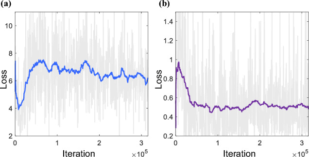
Evolution of a generator and b discriminator loss during network training iterations
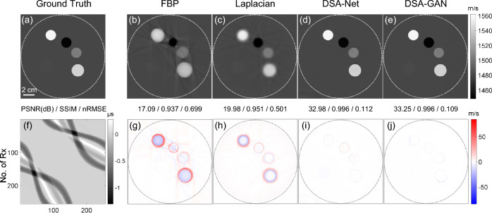
Figure 5 presents the results obtained on the synthetic circle dataset. The results generated by DSA-GAN demonstrate the lowest overall error level, with almost no deviation within the structure, except for the edges of circular structures. In contrast, the predicted results of DSA-Net not only exhibit significant errors at the edges but also show unstable bias within the structure, particularly noticeable inside the circle with the lowest SOS value. Additionally, compared to the results of DSA-Net, the structures in the images generated by DSA-GAN are clearer with lower noise.
Fig. 5.
Comparison of reconstruction results using different algorithms for a numerical phantom composed of disks. a Ground truth, b FBP, c Laplacian, d DSA-Net, e DSA-GAN, f TOF map as input, g–j show the residual images of b–e with respect to the reference ground truth, respectively
Normal breast phantom dataset
The simple numerical phantoms offer an oversimplified representation of the intricate anatomical structures present in the human female breast. To address this limitation, in this section, we generated a dataset from clinical contrast-enhanced magnetic resonance angiography breast images [34, 35]. These images encompass 3D data obtained from the breasts of three healthy women, where the breast density levels were classified into three categories: scattered areas of fibro-glandular density, heterogeneously dense, and extremely dense. Following a rigorous data cleaning process, we obtained 579, 275, and 276 coronal slices for the three breasts, respectively. To create the acoustic breast phantoms for our USCT studies, we assigned specific acoustic parameters to different tissue structures as outlined in Table 2. Ultimately, we amassed a total of 4520 images, with 3612 images allocated for training purposes and the remaining 908 images designated for testing.
Table 2.
Setting of SOS for each tissue in the numerical breast phantom dataset
| Tissue | Speed-of-sound value (m/s) | |||
|---|---|---|---|---|
| 1 | 2 | 3 | 4 | |
| Background | 1480 | 1480 | 1480 | 1480 |
| Fibro-glandular | ||||
| Fat | ||||
| Skin | ||||
| Blood vessel | ||||
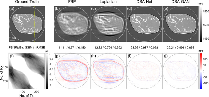
Figure 6 illustrates the results of the test data from breasts with scattered areas of fibro-glandular density. The reconstruction results of FBP can provide coarse shape information and approximate spatial localization. The Laplacian method provides relatively accurate structure information, but there are noticeable artifacts in the low SOS regions around the compressed breast. This may be due to acoustic waves prioritizing the high SOS regions, leading to advoidance of the low SOS regions during the iterative process. Both DSA-GAN and DSA-Net generate results similar to the ground truth image. The prediction results of DSA-Net show a relatively high SOS value for the glandular regions, while the errors in the image generated by DSA-GAN are distributed more uniformly and relatively low.
Fig. 6.
Comparison of reconstruction results using different algorithms for a breast phantom mimicking the scattered area of fibro-glandular density
The SOS value profiles along the yellow dashed lines in Fig. 6 are presented in Fig. 7. It is evident that the FBP reconstruction result deviates significantly from the ground truth and can only roughly reflect the trend of SOS changes. The Laplacian method provides relatively accurate SOS values in the glandular regions; however, it introduces blurring effects along the boundaries, resulting in an expanded glandular area. As a result, significant deviations in SOS values are observed in the background fat regions. The predicted result of DSA-Net closely approximates the true SOS distribution, although some fluctuations are present in the fat region, and there is an overestimation of approximately 5 m/s at the glandular location. The DSA-GAN-generated results demonstrate the best performance, with the closest approximation to the ground truth values. It exhibits deviations in SOS of approximately 2 m/s at the glandular location and an almost identical distribution of SOS in the background fat regions.
Fig. 7.
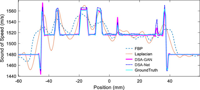
Quantitative SOS values along the yellow dashed line in Fig. 6a
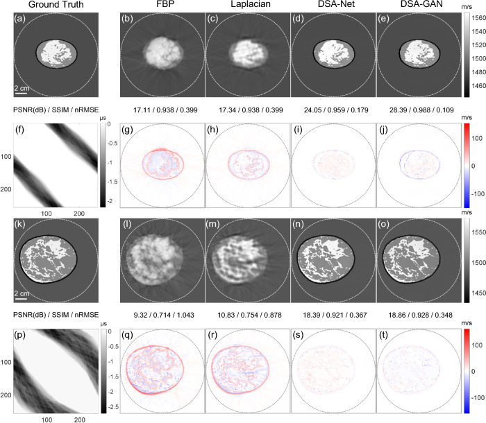
In addition, tests were also conducted on breast phantoms simulating heterogeneously dense and extremely dense tissue compositions, as depicted in Fig. 8. Despite the inherent challenges posed by denser glandular distributions in these phantoms, DSA-GAN consistently demonstrates superior performance and achieved the most accurate reconstructions among all the evaluated algorithms. However, it is worth noting that some errors are primarily concentrated along the edges, while the SOS values in the main regions exhibit high accuracy.
Fig. 8.
Comparative analysis of reconstruction results using different algorithms for breast phantoms mimicking heterogeneously dense breasts (top two rows) and extremely dense breasts (bottom two rows)
Breast cancer phantom dataset
Furthermore, we used a custom-made dataset by inserting lesions into breast slices to simulate and obtain the breast cancer phantom dataset. The breast slices were obtained from a dataset consisting of dedicated breast CT images of 150 clinical patients. Semiautomatic image classification methods as described in [36, 37] were used to classify the images into fibro-glandular, fat, skin, and air. The breast diameters in the dataset ranged from 57 mm to 138 mm, and the glandular fraction by mass ranged from 0.5% to 63.9. The breast lesions [38, 39] were obtained from 50 breast cancer models obtained by segmenting 3D patient breast tomosynthesis images, eight models obtained by segmenting whole body and breast cadaver CT images, and 80 models based on a mathematical algorithm. Finally, the breast cancer phantom dataset was created by randomly inserting tumor slices into each coronal section of the breast with their original sizes to simulate the cross-sectional distribution of breast cancer in patients. We then used the SOS settings [40] listed in Table 3. Finally, the dataset consisted of 42577 slices, of which 34002 were used for training and 8575 were used for testing.
Table 3.
Setting of SOS values for each tissue in the synthetic breast tumor phantom dataset
| Tissue | Background | Skin | Fat | Fibro- glandular |
Benign Tumor |
Malignant Tumor |
|---|---|---|---|---|---|---|
| SOS value (m/s) | 1480 |
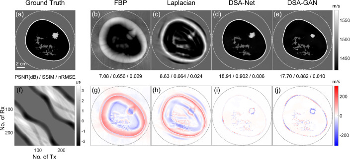
Figure 9 illustrates a performance comparison of different reconstruction algorithms on the breast tumor phantom test set. DSA-GAN achieves a significant improvement in PSNR, increasing from 7.08 dB to 17.70 dB, while DSA-Net performs even better with an increase to 18.91 dB when compared to the FBP results. The estimated tumor sizes for FBP, Laplacian, DSA-Net, and DSA-GAN are approximately , , , and , respectively, compared to the ground truth size of . These results indicate that both the DSA-GAN and DSA-Net methods are able to more accurately reconstruct the structure and size of the tumor.
Fig. 9.
Comparison of reconstruction results of different algorithms for breast phantoms mimicking breast with tumors
The average SOS value inside the tumor is 1544 m/s according to the ground truth. The results obtained using the FBP, Laplacian, DSA-Net, and DSA-GAN methods have average SOS values of approximately 1465 m/s, 1494 m/s, 1535.5 m/s, and 1541.6 m/s, respectively. These values demonstrate that the SOS value obtained by DSA-GAN is the closest to the ground truth value of 1544 m/s. Additionally, it is noteworthy that the reconstruction results of DSA-GAN exhibit clearer and more defined edges compared to the results obtained using DSA-Net.
Computational cost
The computational complexity of Laplacian and Bayesian methods primarily originates from the forward process, with ray-tracing being the most time-consuming step, resulting in a complexity expressed as . In contrast, the complexity of DSA-GAN is mainly dependent on the size of the input TOF map, which is of the order . This complexity is significantly lower compared to the complexity observed in the bent-ray methods.
Table 4 presents the reconstruction time for a image using different algorithms under the same computing environment as stated in Sect. 2.2.3. The FBP method exhibits a short reconstruction time of 0.17 s, but its reconstruction quality is poor. On the other hand, the Laplacian method achieves relatively better reconstruction quality compared to FBP, but it has a longer reconstruction time of 495.6 s, significantly higher than other methods. In contrast, both DSA-GAN and DSA-Net only require passing through the generator network, resulting in a prediction time of 0.05 s for both methods, making them the fastest among all the methods.
Table 4.
Comparison of reconstruction time for a image using different algorithms
| Algorithm | FBP | Laplacian | DSA-Net | DSA-GAN |
|---|---|---|---|---|
| Time | 0.17 s | 495.6 s | 0.05 s | 0.05 s |
Discussion and conclusions
In this paper, we introduced a novel network called DSA-GAN, which integrates the principles of conditional WGAN and Pix2Pix. DSA-GAN effectively accomplishes direct mapping from TOF data in the sensor domain to quantitative SOS images, eliminating the need for incorporating physical knowledge in the conventional inverse problem reconstruction process. Furthermore, DSA-GAN outperforms conventional approaches in terms of both speed and image quality, making it the fastest and yielding the highest quality results. This notable performance advantage holds promise for facilitating the future implementation of real-time whole breast imaging in USCT.
The WGAN with a gradient penalty offers several advantages over the original GAN, leading to improved network training and addressing the mode collapse problem. By introducing the gradient penalty, the convergence during network training is accelerated, ensuring a smoother and more stable learning process. Furthermore, mode collapse mitigation in DSA-GAN allows it to capture intricate features and variations in the TOF map, crucial for accurate SOS image reconstruction.
The proposed DSA-GAN in this paper is a purely data-driven algorithm that relies on a substantial amount of diverse datasets for training. These datasets should encompass various conditions, including different distributions, sizes, sound speed contrasts, and positions of tumors. Only with such comprehensive data can accurate reconstruction of SOS images be achieved without prior knowledge. However, acquiring such extensive data poses challenges in clinical application. To tackle this issue, one approach is to employ data augmentation techniques to generate synthetic data that can be used to train the network. Additionally, incorporating transfer learning shows promise in enhancing the algorithm’s performance. By leveraging pretrained models or knowledge from related domains, the network can benefit from previous learning experiences. By combining the constraints derived from physical models with data-driven approaches, the accuracy and generalization capability of the reconstruction results can be further improved. This integration also facilitates better comprehension and interpretation of the network outputs, making them more accessible for analysis and understanding.
Funding
This work was supported by the National Natural Science Foundation of China (Grant Nos. 62122072, 12174368, and 61705216), the National Key R & D Program of China (Grant No. 2022YFA1404400), the Anhui Provincial Science and Technology Department (Grant Nos. 202203a07020020 and 18030801138), and the Research Fund of the University of Science and Technology of China (YD2090002015).
Declarations
Conflict of interest
The authors declare that they have no conflict of interest.
Ethical approval
This article does not contain any studies with human participants or animals performed by any of the authors.
Footnotes
Publisher's Note
Springer Nature remains neutral with regard to jurisdictional claims in published maps and institutional affiliations.
References
- 1.Giaquinto AN, Sung H, Miller KD, Kramer JL, Newman LA, Minihan A, et al. Breast cancer statistics, 2022. CA Cancer J Clin. 2022;72(6):524–541. doi: 10.3322/caac.21754. [DOI] [PubMed] [Google Scholar]
- 2.Weiss A, Chavez-MacGregor M, Lichtensztajn DY, Yi M, Tadros A, Hortobagyi GN, et al. Validation study of the American Joint Committee on Cancer eighth edition prognostic stage compared with the anatomic stage in breast cancer. JAMA Oncol. 2018;4(2):203–209. [DOI] [PMC free article] [PubMed]
- 3.Boyd NF, Guo H, Martin LJ, Sun LM, Stone J, Fishell E, et al. Mammographic density and the risk and detection of breast cancer. N Engl J Med. 2007;356(3):227–236. doi: 10.1056/NEJMoa062790. [DOI] [PubMed] [Google Scholar]
- 4.O’Flynn EAM, Fromageau J, Ledger AE, Messa A, D’Aquino A, Schoemaker MJ, et al. Ultrasound tomography evaluation of breast density: a comparison with noncontrast magnetic resonance imaging. Invest Radiol. 2017;52(6):343–348. doi: 10.1097/RLI.0000000000000347. [DOI] [PMC free article] [PubMed] [Google Scholar]
- 5.Wiskin J, Malik B, Pirshafiey N, Klock J. Limited view reconstructions with transmission ultrasound tomography: clinical implications and quantitative accuracy. In: Medical imaging 2020: ultrasonic imaging and tomography. vol. 11319. Bellingham: SPIE; 2020. p. 167–174.
- 6.Andre MP, Barker C, Sekhon N, Wiskin J, Borup DT, Callahan K. Pre-clinical experience with full-wave inverse-scattering for breast imaging. In: Acoustical Imaging. vol. 29. Dordrecht: Springer; 2008. p. 73–80.
- 7.Ali R, Hsieh S, Dahl J. Open-source gauss-newton-based methods for refraction-corrected ultrasound computed tomography. In: Medical imaging 2019: ultrasonic imaging and tomography. vol. 10955. Bellingham: SPIE; 2019. p. 39–52.
- 8.Huthwaite P, Simonetti F. High-resolution imaging without iteration: a fast and robust method for breast ultrasound tomography. J Acoust Soc Am. 2011;130(3):1721–1734. doi: 10.1121/1.3613936. [DOI] [PubMed] [Google Scholar]
- 9.Lucka F, Perez-Liva M, Treeby BE, Cox BT. High resolution 3D ultrasonic breast imaging by time-domain full waveform inversion. Inverse Probl. 2022;38(2):025008. doi: 10.1088/1361-6420/ac3b64. [DOI] [Google Scholar]
- 10.Vishnevskiy V, Rau R, Goksel O. Deep variational networks with exponential weighting for learning computed tomography. In: Proceeding of MICCAI. vol. 11769. Cham: Springer; 2019. p. 310–318.
- 11.Vishnevskiy V, Sanabria SJ, Goksel O. Image reconstruction via variational network for real-time hand-held sound-speed imaging. In: Proceeding of MLMIR. vol. 11074. Cham: Springer; 2018. p. 120–128.
- 12.Bernhardt M, Vishnevskiy V, Rau R, Goksel O. Training variational networks with multidomain simulations: speed-of-sound image reconstruction. IEEE Trans Ultrason Ferroelectr Freq Control. 2020;67(12):2584–2594. doi: 10.1109/TUFFC.2020.3010186. [DOI] [PubMed] [Google Scholar]
- 13.Fan Y, Ying L. Solving traveltime tomography with deep learning. Commun Math Stat. 2023;11:3–19. doi: 10.1007/s40304-022-00329-z. [DOI] [Google Scholar]
- 14.Qu X, Ren C, Yan G, Zheng D, Tang W, Wang S, et al. Deep-learning-based ultrasound sound-speed tomography reconstruction with Tikhonov pseudo-inverse priori. Ultrasound Med Biol. 2022;48(10):2079–2094. doi: 10.1016/j.ultrasmedbio.2022.05.033. [DOI] [PMC free article] [PubMed] [Google Scholar]
- 15.Fan Y, Wang H, Gemmeke H, Hesser J. MI-Net: a deep network for non-linear ultrasound computed tomography reconstruction. In: Proceeding of IEEE International Ultrasonics Symposium. Piscataway: IEEE 2020;1–3.
- 16.Fan Y, Wang H, Gemmeke H, Hopp T, Hesser J. DDN: dual domain network architecture for non-linear ultrasound transmission tomography reconstruction. In: Medical imaging 2021: ultrasonic imaging and tomography. vol. 11602. Bellingham: SPIE 2021;40–45.
- 17.Zhao W, Wang H, Gemmeke H, van Dongen KWA, Hopp T, Hesser J. Ultrasound transmission tomography image reconstruction with a fully convolutional neural network. Phys Med Biol. 2020;65(23):235021. doi: 10.1088/1361-6560/abb5c3. [DOI] [PubMed] [Google Scholar]
- 18.Fan Y, Wang H, Gemmeke H, Hopp T, Dongen KV, Hesser J. Memory-Efficient Neural Network For Non-Linear Ultrasound Computed Tomography Reconstruction. In: Proceeding of IEEE international symposium on biology image. Piscataway: IEEE 2021;429–432.
- 19.Prasad S, Almekkawy M. DeepUCT: complex cascaded deep learning network for improved ultrasound tomography. Phys Med Biol. 2022;67(6):065008. doi: 10.1088/1361-6560/ac5296. [DOI] [PubMed] [Google Scholar]
- 20.Ronneberger O, Fischer P, Brox T. U-Net: Convolutional networks for biomedical image segmentation. In: Proceeding of MICCAI. vol. 9351. Cham: Springer 2015; 234–241.
- 21.Fan YL, Wang HJ, Gemmeke H, Hopp T, Hesser J. Model-data-driven image reconstruction with neural networks for ultrasound computed tomography breast imaging. Neurocomputing. 2022;467:10–21. doi: 10.1016/j.neucom.2021.09.035. [DOI] [Google Scholar]
- 22.Zhu B, Liu JZ, Cauley SF, Rosen BR, Rosen MS. Image reconstruction by domain-transform manifold learning. Nature. 2018;555(7697):487–492. doi: 10.1038/nature25988. [DOI] [PubMed] [Google Scholar]
- 23.Goodfellow IJ, Pouget-Abadie J, Mirza M, Xu B, Warde-Farley D, Ozair S, et al. Generative adversarial nets. In: Proceeding of NIPS. vol. 2. New York: Curran Associates 2014;2672–2680.
- 24.Arjovsky M, Chintala S, Bottou L. Wasserstein generative adversarial networks. In: Proceeding of ICML. New York: PMLR 2017;214–223.
- 25.Gulrajani I, Ahmed F, Arjovsky M, Dumoulin V, Courville A. Improved Training of Wasserstein GANs. In: Proceeding of NIPS. vol. 30. New York: Curran associates 2017;5769–5779.
- 26.Isola P, Zhu JY, Zhou TH, Efros AA. Image-to-image translation with conditional adversarial networks. In: Proceeding of CVPR. Piscataway: IEEE 2017;1125–1134.
- 27.Mirza M, Osindero S. Conditional generative adversarial nets. Preprint at https://arxiv.org/abs/1411.1784.
- 28.Simonyan K, Zisserman A. Very deep convolutional networks for large-scale image recognition. Preprint at https://arxiv.org/abs/1409.1556.
- 29.Hinton GE, Salakhutdinov RR. Reducing the dimensionality of data with neural networks. Science. 2006;313(5786):504–507. doi: 10.1126/science.1127647. [DOI] [PubMed] [Google Scholar]
- 30.Hu J, Shen L, Albanie S, Sun G, Wu E. Squeeze-and-excitation networks. IEEE Trans Pattern Anal Mach Intell. 2020;42:2011–2023. doi: 10.1109/TPAMI.2019.2913372. [DOI] [PubMed] [Google Scholar]
- 31.Roy AG, Navab N, Wachinger C. Recalibrating fully convolutional networks with spatial and channel “squeeze and excitation” blocks. IEEE Trans Med Imaging. 2019;38:540–9. [DOI] [PubMed]
- 32.Maas AL, Hannun AY, Ng AY. Rectifier nonlinearities improve neural network acoustic models. In: Proceeding of ICML. vol. 28. New York: PMLR 2013;p. 3.
- 33.Kak AC, Slaney M. Principles of computerized tomographic imaging. Philadelphia: SIAM; 2001. [Google Scholar]
- 34.Lou Y, Zhou W, Matthews T, Appleton C, Anastasio M. Generation of anatomically realistic numerical phantoms for photoacoustic and ultrasonic breast imaging. J Biomed Opt. 2017;4:041015. doi: 10.1117/1.JBO.22.4.041015. [DOI] [PMC free article] [PubMed] [Google Scholar]
- 35.Lou Y. Optical and acoustic breast phantoms. Harvard Dataverse 10.7910/DVN/NZBJOC.
- 36.Mettivier G, Sarno A, Franco Fd, Bliznakova K, Bliznakov Z, Hernandez AM, et al. The Napoli-Varna-Davis project for virtual clinical trials in X-ray breast imaging. In: Proceeding of IEEE nuclear science symposium and medicine image conference. Piscataway: IEEE 2019;1–5.
- 37.Sarno A, Mettivier G, di Franco F, Varallo A, Bliznakova K, Hernandez AM, et al. Dataset of patient-derived digital breast phantoms for in silico studies in breast computed tomography, digital breast tomosynthesis, and digital mammography. Med Phys. 2021;48(5):2682–2693. doi: 10.1002/mp.14826. [DOI] [PubMed] [Google Scholar]
- 38.Bliznakova K, Dukov N, Feradov F, Gospodinova G, Bliznakov Z, Russo P, et al. Development of breast lesions models database. Phys Med. 2019;64:293–303. doi: 10.1016/j.ejmp.2019.07.017. [DOI] [PubMed] [Google Scholar]
- 39.Dukov N, Bliznakova K, Feradov F, Ridlev I, Bosmans H, Mettivier G, et al. Models of breast lesions based on three-dimensional X-ray breast images. Phys Med. 2019;57:80–87. doi: 10.1016/j.ejmp.2018.12.012. [DOI] [PubMed] [Google Scholar]
- 40.Li C, Duric N, Littrup P, Huang L. In vivo breast sound-speed imaging with ultrasound tomography. Ultrasound Med Biol. 2009;35(10):1615–1628. doi: 10.1016/j.ultrasmedbio.2009.05.011. [DOI] [PMC free article] [PubMed] [Google Scholar]


