Getting Started with the IDG KMC Datasets and Tools

Eryk Kropiwnicki; Jessica Binder; Jeremy Yang; Jayme Holmes; Alexander Lachmann; Daniel J B Clarke; Timothy Sheils; Keith Kelleher; Vincent Metzger; Cristian G Bologa; Tudor I Oprea; Avi Ma’ayan

doi:10.1002/cpz1.355

. Author manuscript; available in PMC: 2024 Jan 15.

Published in final edited form as: Curr Protoc. 2022 Jan;2(1):e355. doi: 10.1002/cpz1.355

Getting Started with the IDG KMC Datasets and Tools

Eryk Kropiwnicki ^1,^⧪, Jessica Binder ^2,^⧪, Jeremy Yang ², Jayme Holmes ², Alexander Lachmann ¹, Daniel J B Clarke ¹, Timothy Sheils ³, Keith Kelleher ³, Vincent Metzger ², Cristian G Bologa ², Tudor I Oprea ^2,^*, Avi Ma’ayan ^1,^*

PMCID: PMC10789444 NIHMSID: NIHMS1767466 PMID: 35085427

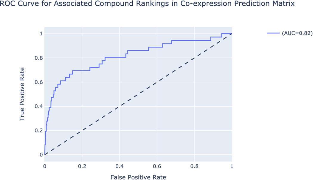
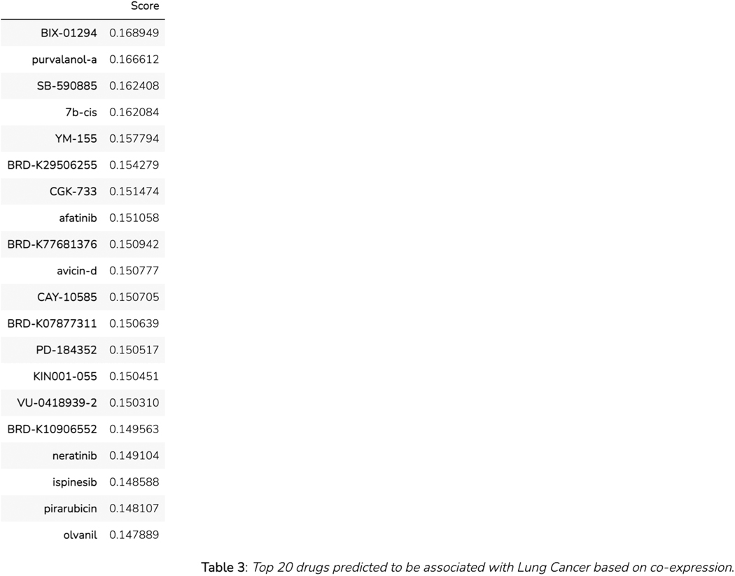
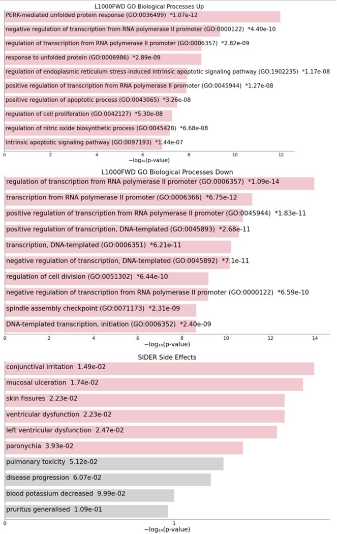
Abstract

The Illuminating the Druggable Genome (IDG) consortium is a National Institutes of Health (NIH) Common Fund program designed to enhance our knowledge of understudied proteins. More specifically, proteins unannotated within the three most commonly drug-targeted protein families: G-protein coupled receptors, ion channels, and protein kinases. Since 2014, the IDG Knowledge Management Center (IDG-KMC) has generated several open-access datasets and resources that jointly serve as a highly translational machine learning ready knowledgebase focused on human protein-coding genes and their products. The goal of the IDG-KMC is to develop comprehensive integrated knowledge for the druggable genome to illuminate the uncharacterized or poorly annotated portion of the druggable genome. The tools derived from the IDG-KMC provide either user-friendly visualizations or ways to impute the knowledge about potential targets using machine learning strategies. In the following protocols, we describe how to use each web-based tool for researchers to accelerate illumination in understudied proteins.

Basic Protocol 1: Interacting with the Pharos user interface

Basic Protocol 2: Accessing the data in Harmonizome

Basic Protocol 3: The ARCHS4 resource

Basic Protocol 4: Making predictions about gene function with PrismExp

Basic Protocol 5: Using Geneshot to illuminate knowledge about under-studied targets

Basic Protocol 6: Exploring understudied targets with TIN-X

Basic Protocol 7: Interacting with the DrugCentral user interface

Basic Protocol 8: Estimating Anti-SARS-CoV-2 activities with DrugCentral REDIAL-2020

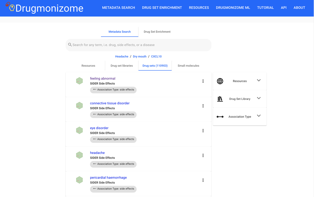
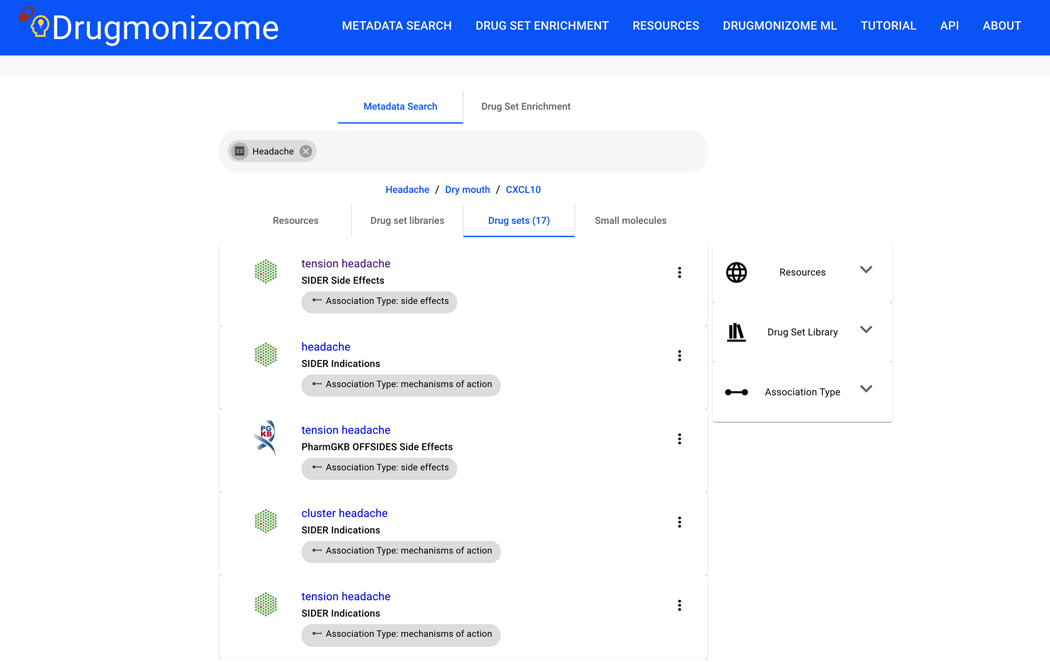
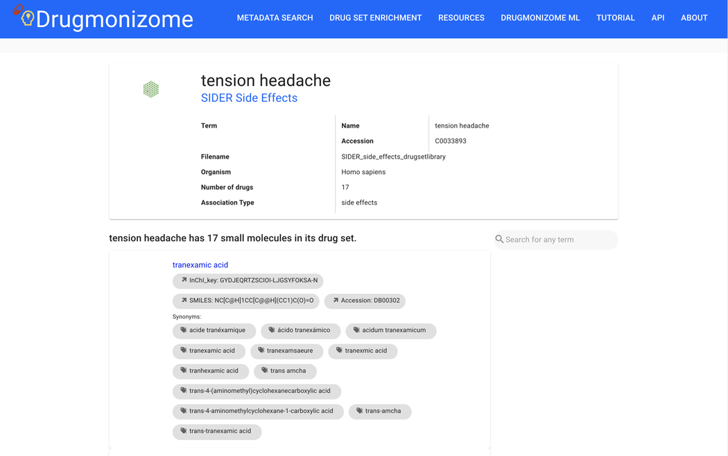
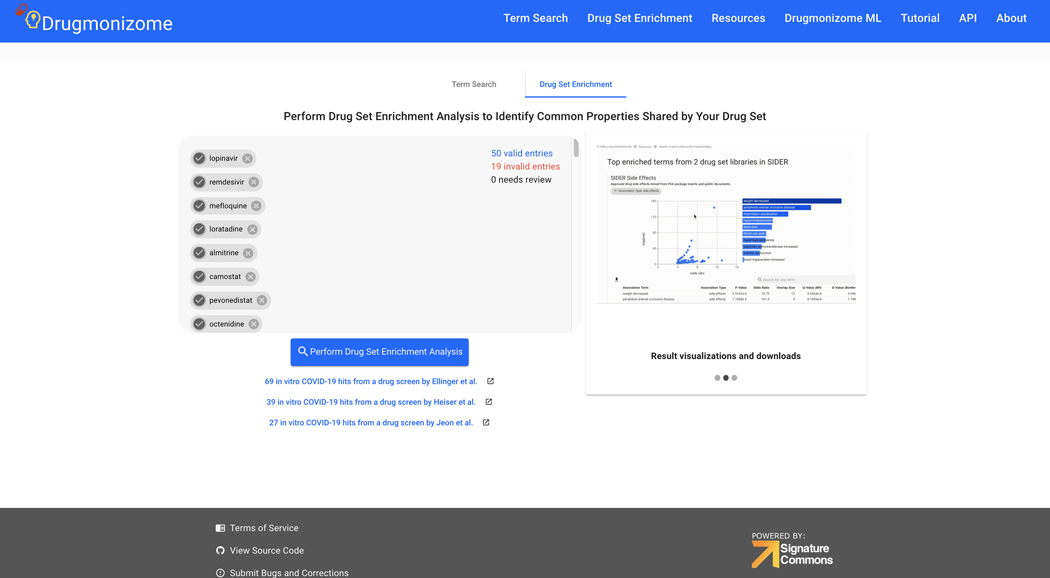
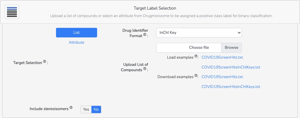
Basic Protocol 9: Drug Set Enrichment Analysis using Drugmonizome

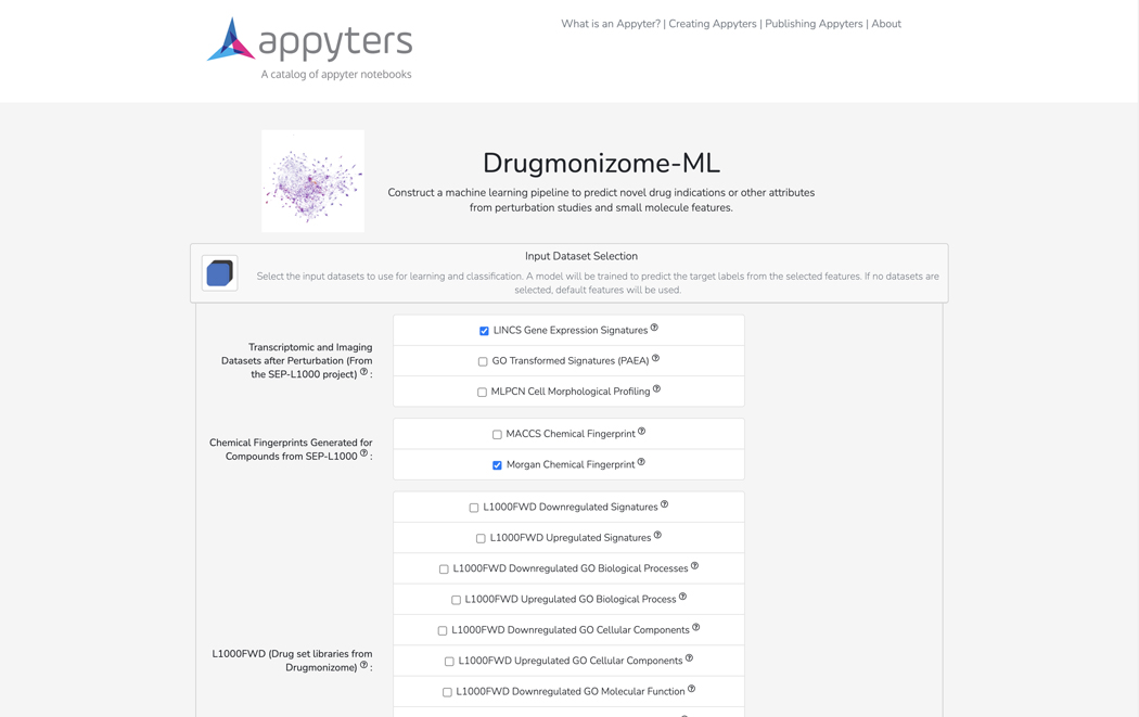
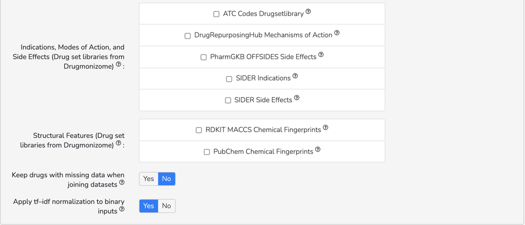
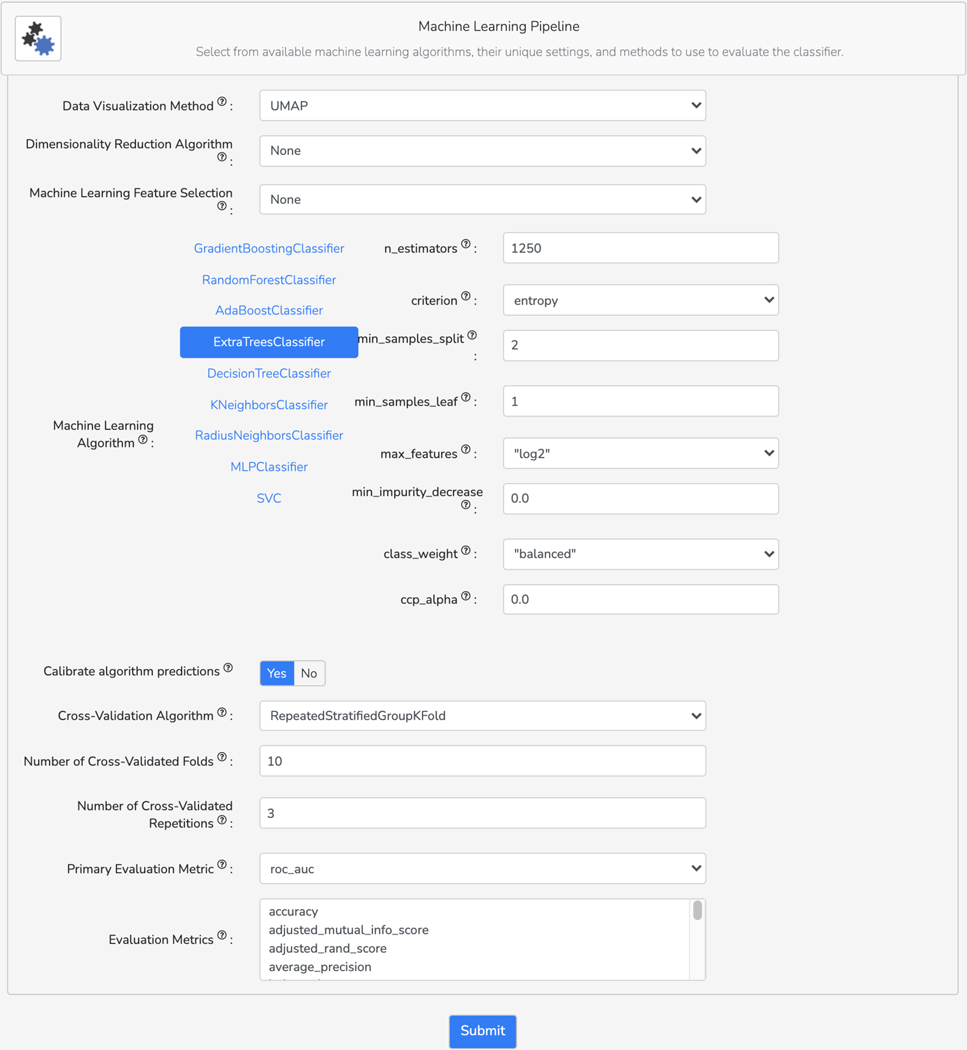
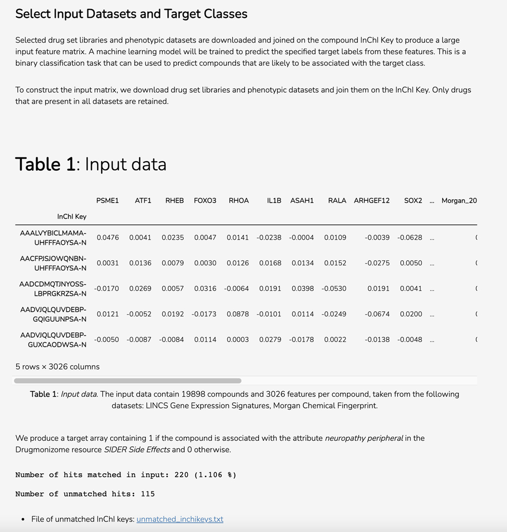
Basic Protocol 10: The Drugmonizome-ML Appyter

Basic Protocol 11: The Harmonizome-ML Appyter

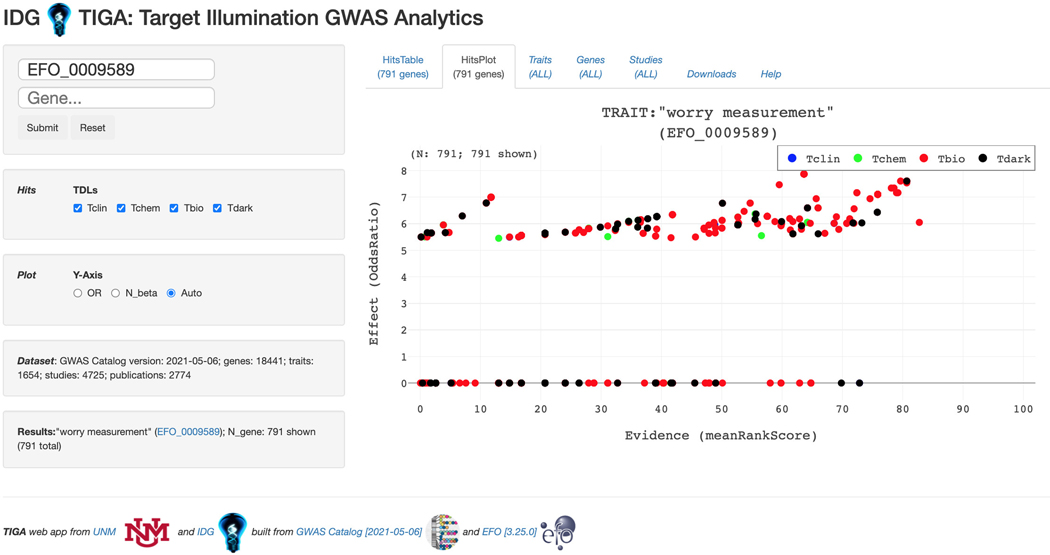
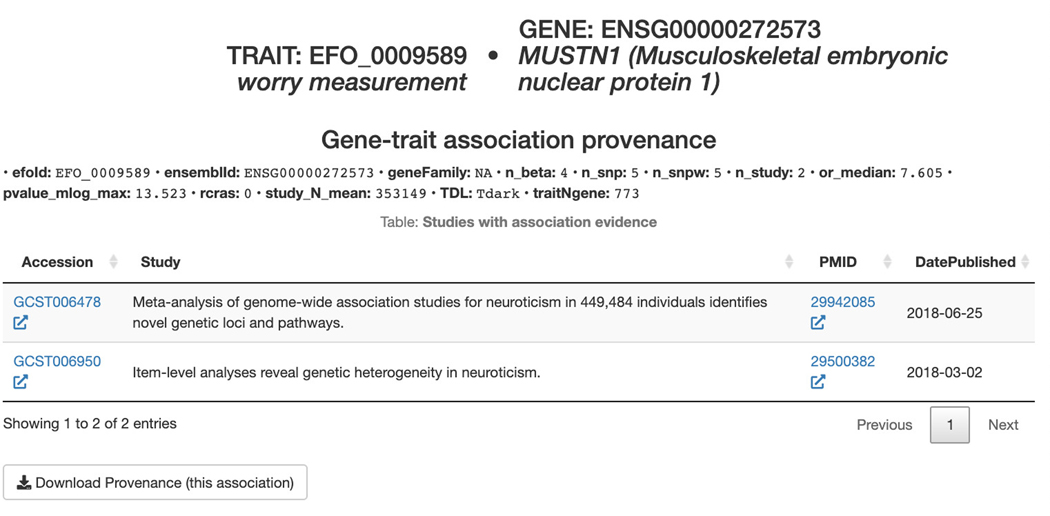
Basic Protocol 12: GWAS target illumination with TIGA

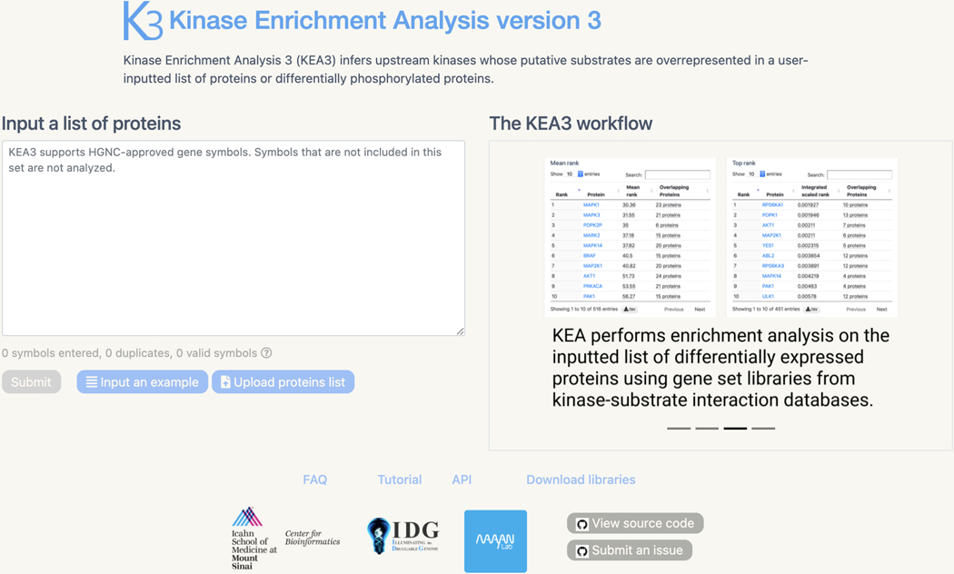
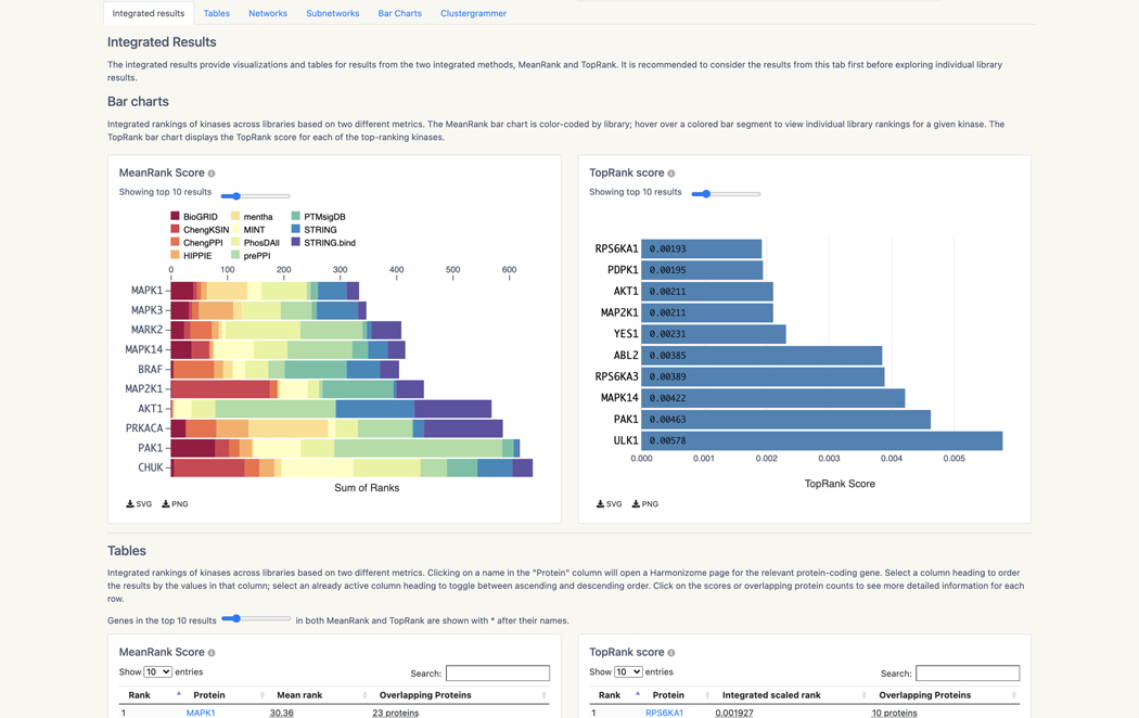
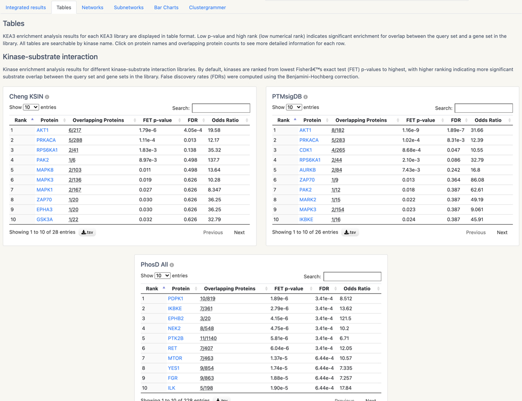
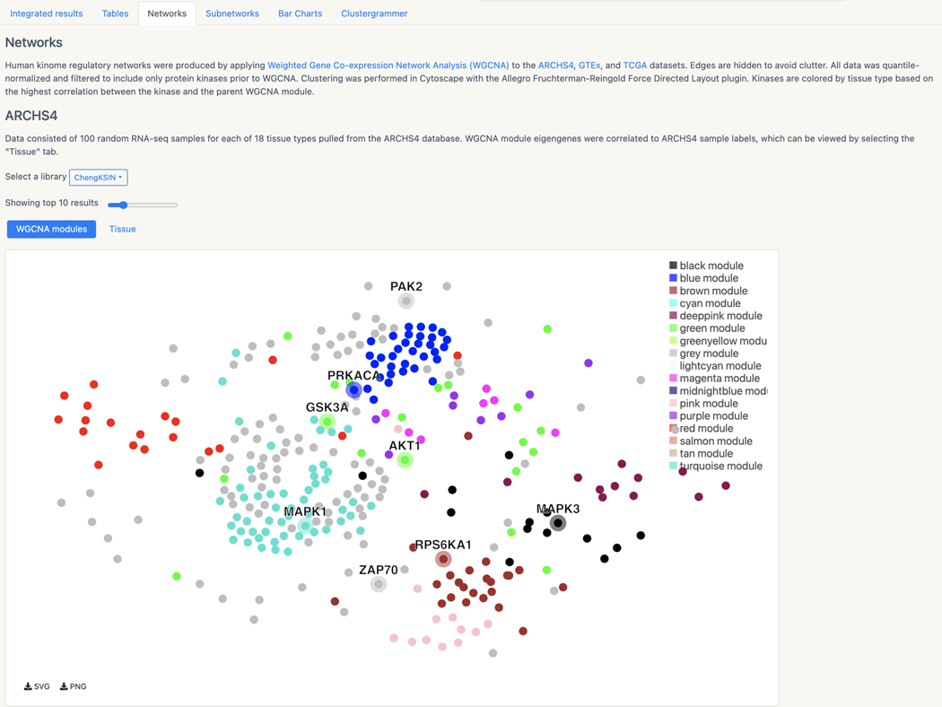
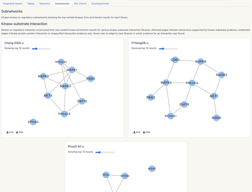
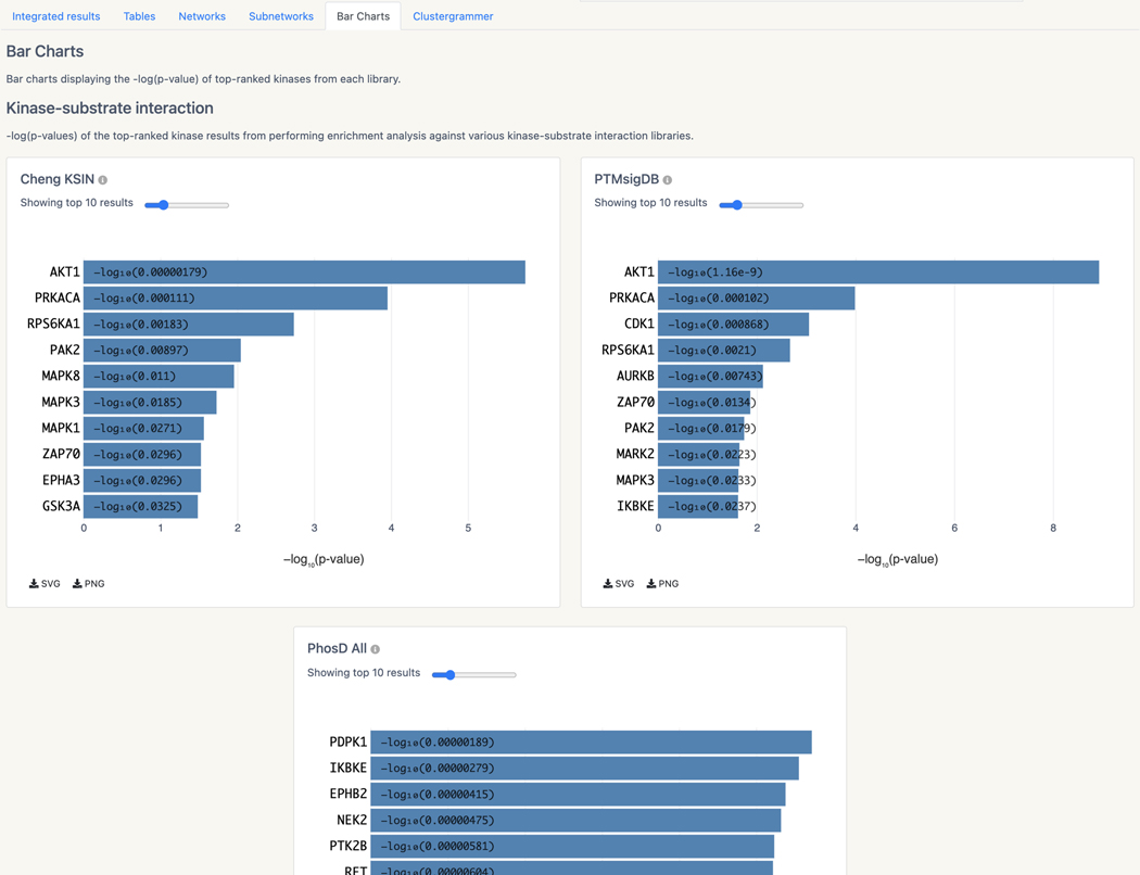
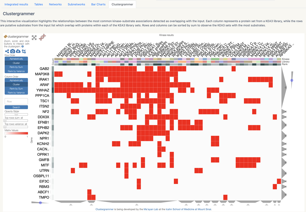
Basic Protocol 13: Prioritizing kinases for lists of proteins and phosphoproteins with KEA3

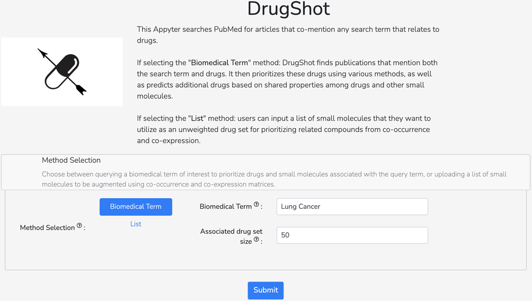
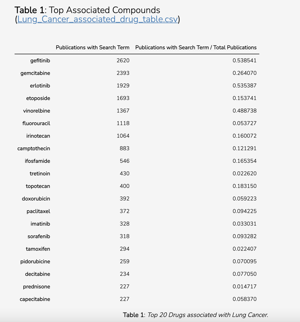
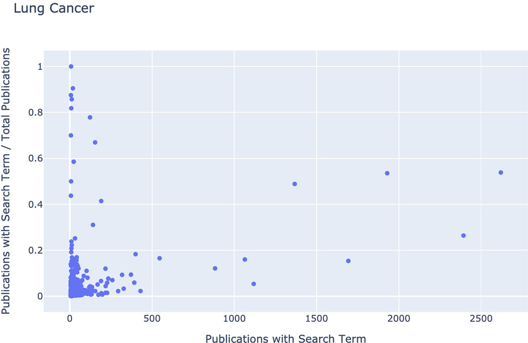
Basic Protocol 14: Converting PubMed searches to drug sets with the DrugShot Appyter

Keywords: bioinformatics, druggable genome, drug targets, disease ontology, drug discovery, data visualization, web applications

INTRODUCTION

There are approximately 25,000 protein-coding genes (Venter et al., 2001) in the human genome. Abnormal protein expression is associated with many human diseases, which makes proteins critical targets for therapeutic agents. Approximately 15% of protein-coding genes are considered part of the “druggable genome”. This means that these proteins can modulate cellular behavior when targeted by experimental small molecule compounds (Hopkins and Groom, 2002; Lipinski et al., 2001; Russ and Lampel, 2005; Johns et al., 2012). Moreover, only a few hundred targets represent the existing clinical pharmacopeia, leaving a massive swath of pharmacology that remains unexploited. Therefore, 85% of druggable proteins remain to be explored as potential therapeutic targets. Much of the druggable genome encodes three critical protein families: non-olfactory G-protein-coupled receptors (GPCRs), ion channels, and protein kinases. Critically, we currently lack crucial knowledge about the function of many proteins from these families and their roles in health and disease. A better understanding of these proteins, structurally or functionally, could shed light on new avenues of investigation for basic science and therapeutic discovery (Oprea et al., 2018).

In this article, we provide several protocols to guide users through the use of IDG tools that accomplish specific computational tasks related to illuminating the druggable genome. In Basic Protocol 1, we describe how users can query the Pharos web interface (Sheils et al., 2021) to search for data related to gene targets. Basic Protocol 2 explains how to use Harmonizome (Rouillard et al., 2016), a web application that stores gene-attribute associations from various sources that can be readily visualized and leveraged for machine learning. Basic Protocol 3 describes ARCHS4 (Lachmann et al., 2018), a web application that provides easy access to RNA-sequencing data from human and mouse experiments and also includes gene landing pages for all human genes with gene function predictions based on mRNA co-expression. Basic Protocol 4 describes PrismEXP (Lachmann et al., 2021), a machine learning Appyter (Clarke et al., 2021) that improves gene function predictions from gene co-expression correlation data by sharding the global gene-gene co-expression matrix used by ARCHS4. Basic Protocol 5 teaches the user how to use Geneshot (Lachmann et al., 2019), a web application that facilitates querying of biomedical search terms to retrieve prioritized lists of genes related to the search terms. In Basic Protocol 6 we introduce TIN-X (Cannon et al., 2017), the Target Importance and Novelty eXplorer. We demonstrate to users how to query and explore interesting disease-target associations based on novelty and importance metrics derived from natural language processing (NLP) of PubMed abstracts. Basic Protocol 7 describes DrugCentral (Avram et al., 2021), a comprehensive database of approved drugs that includes information relating to drug side effects, mode of action, indications, pharmacologic action, and other information. Basic Protocol 8 explains REDIAL-2020 (Kc et al., 2021), an ensemble machine learning platform that extends the information available in DrugCentral to predict drugs and small molecules that may have anti-SARS-CoV-2 activity. In Basic Protocol 9 we discuss Drugmonizome (Kropiwnicki et al., 2021), a web application that facilitates drug set enrichment analysis and allows users to submit a drug set of interest to retrieve enriched terms that all, or most, of the members of the input set share. Basic Protocol 10 describes Drugmonizome-ML (Kropiwnicki et al., 2021), an Appyter that extends the information available in Drugmonizome to build on-the-fly machine learning models for predicting novel drug and small molecule attributes. In a similar vein, Basic Protocol 11 discusses Harmonizome-ML, an Appyter that enables users to utilize the datasets from Harmonizome to build machine learning models that predict novel gene-attribute associations. Basic Protocol 12 includes a discussion of TIGA (Yang et al., 2021), Target Illumination GWAS Analytics, a tool that summarizes gene-trait associations derived from genome wide association studies (GWAS) with rational and intuitive evidence metrics. In Basic Protocol 13 we describe how users can submit an input list of genes or differentially phosphorylated proteins to KEA3 for kinase enrichment analysis (Kuleshov et al., 2021) to infer kinases associated with the input list. Basic Protocol 14 explains how to use DrugShot, an Appyter that allows for the querying of biomedical search terms to retrieve known and predicted lists of drugs and small molecules related to the query term.

Basic Protocol 1: Interfacing with the Pharos user interface

Pharos is the user interface to the Knowledge Management Center (KMC) for the IDG program, providing facile access to most data types collected by the KMC (Nguyen et al., 2017; Sheils et al., 2020). Given the complexity of the data surrounding any target, efficient and intuitive visualization has been a high priority for users to navigate and summarize search results and rapidly identify patterns. Underlying the interface is a GraphQL API that provides programmatic access to all KMC data, enabling the incorporation of IDG resources with other applications.

Necessary Resources

Hardware

Desktop or a laptop computer, or a mobile device, with a fast Internet connection

Software

An up-to-date web browser such as Google Chrome (https://www.google.com/chrome/), Mozilla Firefox (https://www.mozilla.org/en-US/firefox/), Apple Safari (https://www.apple.com/safari/), or Microsoft Edge (https://www.microsoft.com/en-us/edge).

Protocol steps and annotations

Search Targets

1
Navigate to Pharos (https://pharos.nih.gov).
2
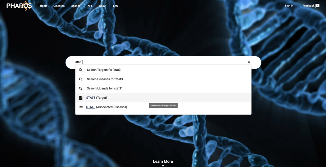
To search for a target, click on the search box on the main page or in the top left corner of subsequent pages. Enter ‘STAT3’. Note that multiple search types are available in the dropdown menu. (Figure 1)
3
It is possible to search by pathway or view a list of diseases or ligands associated with a target. Additionally, pressing enter or return will allow a text-based search, which will return a list of results featuring ‘stat3’ anywhere in the text.
4
Press ‘enter’, ‘return’ or click the magnifying glass icon to search for the ‘stat3’ text string.
5
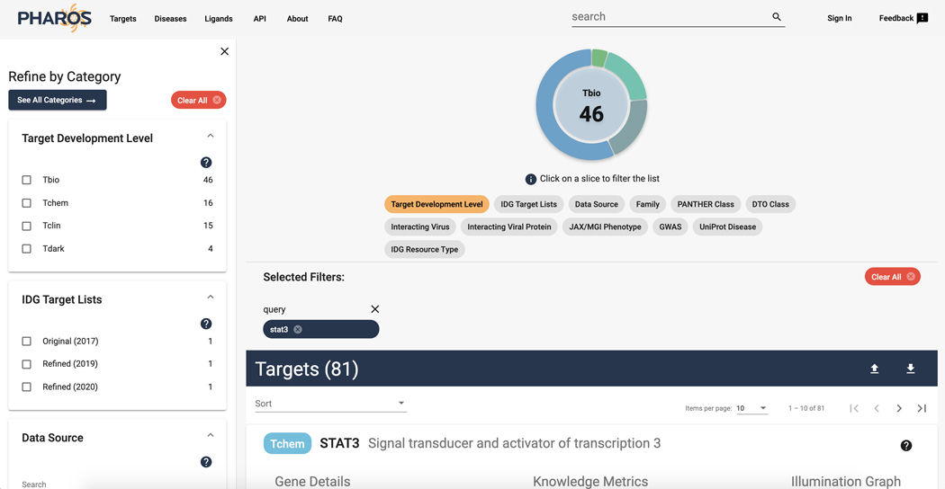
A list of 81 targets is returned, with ‘STAT3’ being at the top of the list. The rest of the targets will have the phrase ‘stat3’ somewhere within the target details. (Figure 2)
6
Click on the STAT3 card to view the target details.

Figure 1. — Typeahead search results for STAT3 scroll or arrow down to view more options.

Figure 2. — Search Targets for STAT3 search results page.

View target details

7
Follow the steps from above, or alternatively, click on the STAT3 (Target) option from the search box auto-complete. This will navigate directly to the STAT3 target details page.
8
The target details page is divided into several sections that highlight an area of knowledge about the target.
9
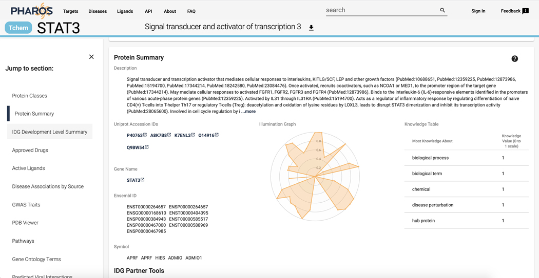
Scroll down to the “Protein Summary” section. A brief description of the target, as well as several identifiers is available. In addition, the central radar plot charts the relative knowledge of a target compared to the rest of TCRD on a 0 to 1 scale. This data is sourced from the Harmonizome, which will be discussed further (Figure 3).
10
Scroll down to the next section, “IDG Development Level Summary”. Displayed here is the current development level . Each level has the criteria listed, as well as links to the data for each property (Figure 4).
11
On the left side panel, click on “Disease Associations by Source”. This will navigate within the page to a section displaying disease associations from a variety of sources.
12
Scroll down to the “Disease Novelty (Tin-x)” section, just below Disease Associations. A scatterplot is visible that shows Tin-x data. This data is explained in Protocol 6. Briefly, it is natural language processed PubMed abstracts that chart a target’s importance to a disease, as well as the novelty of that target to the disease. A dense chart indicates a large amount of knowledge about a target and its disease associations, whereas a sparser chart would indicate that target is not frequently studied and has fewer disease associations (Figure 5).
13
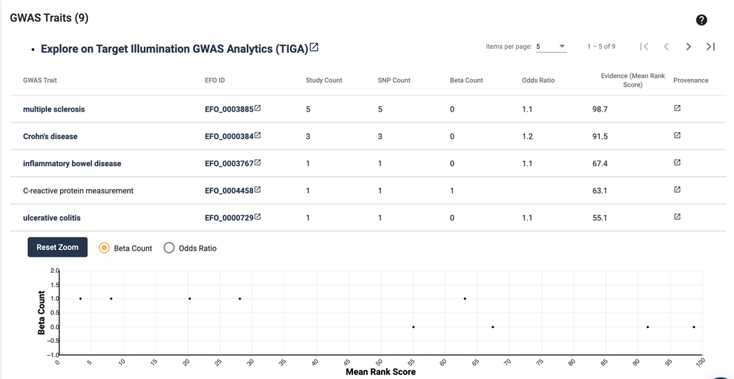
Scroll down to the next section “GWAS Traits”. Here a table of GWAS traits is displayed. This list focuses on scoring and ranking protein-coding genes associated with traits from genome-wide association studies. This allows both the discovery of traits most associated with a target, but also lesser emphasized traits (Figure 6).

Figure 3. — Target details page for STAT3, the radar chart in the center depicts data from Harmonizome.

Figure 4. — IDG development level summary section that shows the current development level, and criteria met. Links provide the ability to view either the original source, or the relevant data in Pharos.

Figure 5. — Scatterplot depicting Tin-x data for STAT3. Hovering over a data point opens up a tooltip, providing novelty and importance data for the disease.

Figure 6. — GWAS traits, and the associated TIGA scatterplot. For a more in depth exploration of this data, click “Explore on Target Illumination GWAS Analytics”.

Finding a list of Understudied targets that share disease associations with STAT3

14
From the STAT3 target details page, click on “Disease Associations by Source” on the left panel.
15
Click on the “Find Similar Targets” button, directly under the panel header (Figure 7).
16
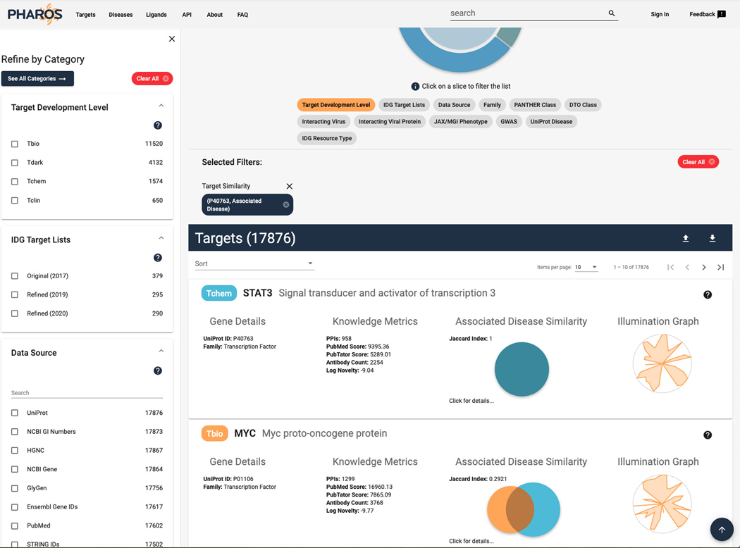
The targets list page is now shown, with a target similarity filter applied, showing 17,876 targets (Figure 8).
17
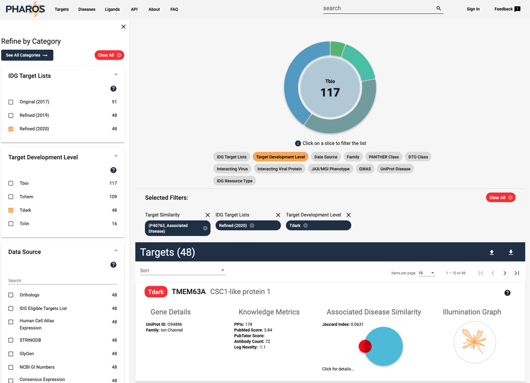
To refine this list for targets of interest to the IDG program (mentioned in Protocol 1), click on the “Refined (2020)” checkbox in the IDG Target Lists filter panel on the left side of the page. The list of targets shown is reduced to 290.
18
To find only dark targets in this list, click the “Tdark” value in the Target Development Level filter panel, returning 48 targets (Figure 9).
19
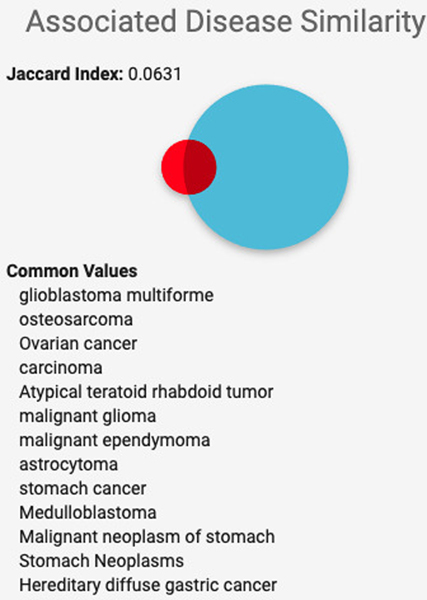
Click on the “click for details…” text on the TMEM63A target card to view a list of associated diseases that this target shares with STAT3 (Figure 10).

Figure 7. — Additional functions available within Pharos are shown within blue buttons. Users can click to browse filtered lists for targets similar to the current target, or associated diseases or ligands.

Figure 8. — List of targets that share associated diseases with STAT3. The Jaccard index is a numerical value of the ratio of overlap between the associated diseases of the target in relation to the original target (STAT3). The Venn diagram is a visual representation of the ratio with the TDL level color coded.

Figure 9. — The target list from Figure 8 filtered to display Target Development Level of Tdark, and on the Refined(2020) IDG target lists. Click on “Click for details…” to view an expanded list of the overlapping values.

Figure 10. — Expanded view of the Associated Disease Similarity section of the target card.

Download target list

20
Click on the downward facing arrow on the right side of the Targets header (Figure 11).
21
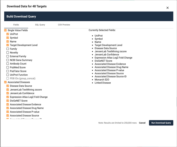
A window will pop open displaying a list of fields that can be selected (Figure 12).
22
Click on the Associated Diseases checkbox. Note that many fields are deactivated, to reduce the overall file size.
23
Click on Name and Target Development Level under the Single Value Fields heading.
24
Click the Run Download Query Button. A file download dialog will open. Depending on the complexity of the target list and the fields selected, it may take some time.
25
After the file is downloaded, this list of targets can be used as a starting point for many of the protocols listed below.

Figure 11. — Target toolbar illustrating the download button on the right side. To the left of the download button is the upload button, which allows for the uploading of custom lists, to explore in the Pharos interface.

Figure 12. — Popup window featuring the query builder which allows for the download of Pharos list data as a csv file. Subsequent tabs display the raw SQL query used to generate the data, as well as a 10 line preview.

GraphQL queries

26
Click on API on the main Pharos header.
27
A code “sandbox” is now visible, allowing testing of GraphQL queries to fetch complex data from Pharos. A distinct feature of GraphQL is the ability of the consumer to determine the exact fields returned from the query, as opposed to a SQL query, where the data returned is determined by the database developer.
28
Click the “Play” button in the top center to run a sample query. A list of Drugs associated with DRD2 is returned.
29
Click on the “Docs” tab on the right side of the page. A menu will open up that displays the queries available, the inputs required, and the responses and properties returned. Click on the “Docs” tab again to close the menu.

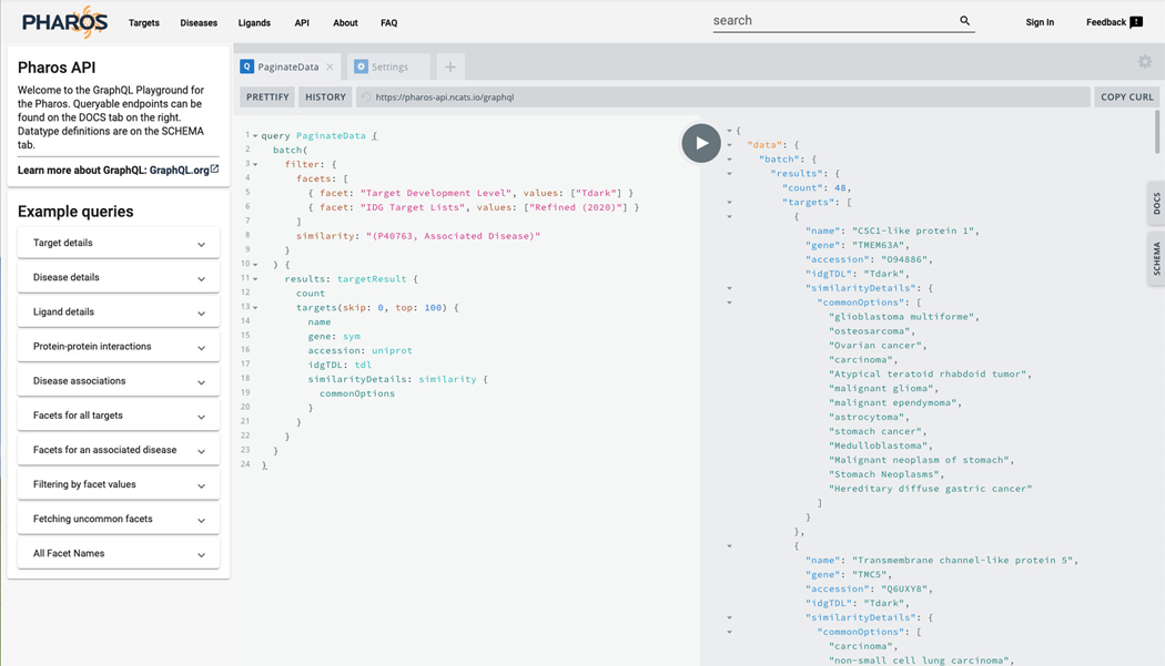
Replace the text in the left column with this query:

query PaginateData {
 batch(
  filter: {
   facets: [
    { facet: “Target Development Level”, values: [“Tdark”] }
    { facet: “IDG Target Lists”, values: [“Refined (2020)”] }
   ]
   similarity: “(P40763, Associated Disease)”
  }
 ) {
  results: targetResult {
   count
   targets(skip: 0, top: 100) {
    name
    gene: sym
    accession: uniprot
    idgTDL: tdl
    similarityDetails: similarity {
     commonOptions
     }
    }
   }
  }
 }

31
Press the play button. This query fetches all Dark targets of interest to the IDG that share associated diseases with STAT3. Returned is the target name, gene symbol, Uniprot id, IDG TDL, and shared associated diseases (Figure 13).

GraphQL sandbox interface. Examples on the left side, and documentation on the right allow for highly customizable data requests.

Entire Relational Database Download Page

32
Navigate to the TCRD website (http://juniper.health.unm.edu/tcrd/).
33
Click on the “Downloads” tab on the navigation bar at the top of the page to be redirected to a table of downloadable files; ex: MySQL dump of the full TCRD (latest.sql.gz).

Basic Protocol 2: Accessing the data in Harmonizome

The Harmonizome resource contains processed datasets detailing functional associations between genes/proteins and their attributes extracted from 66 online resources. The information from the original datasets was distilled into attribute tables that define significant associations between genes and their attributes, where attributes could be other genes, proteins, pathways, cell lines, tissues, experimental perturbations, diseases, phenotypes, drugs, or other entities depending on the dataset. The Harmonizome web application can be accessed from https://maayanlab.cloud/Harmonizome/ (Rouillard et al., 2016).

Necessary Resources

Hardware

Desktop or a laptop computer, or a mobile device, with a fast Internet connection

Software

An up-to-date web browser such as Google Chrome (https://www.google.com/chrome/), Mozilla Firefox (https://www.mozilla.org/en-US/firefox/), Apple Safari (https://www.apple.com/safari/), or Microsoft Edge (https://www.microsoft.com/en-us/edge).
Text editor or development environment of choice, such as Visual Studio (https://visualstudio.microsoft.com/vs/); most updated version of Python
(https://www.python.org/downloads/ ); Python module for Harmonizome (https://maayanlab.cloud/Harmonizome/static/harmonizomeapi.py)

Protocol steps and annotations

Metadata Search

Navigate to the Harmonizome website (https://maayanlab.cloud/Harmonizome/).
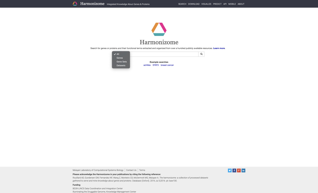
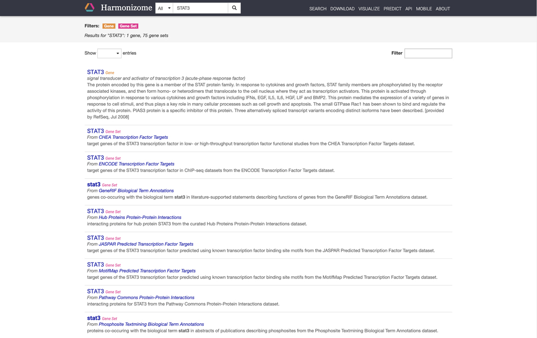
The front page features a search bar where keywords of interest can be input. Click the filter button on the left of the search bar to narrow searches to “genes”, “gene sets”, or “datasets” (Figure 14). Type “STAT3” into the search bar and click the submit button. The results page includes a single gene landing page for STAT3 and 75 gene sets with STAT3 as an attribute (Figure 15).
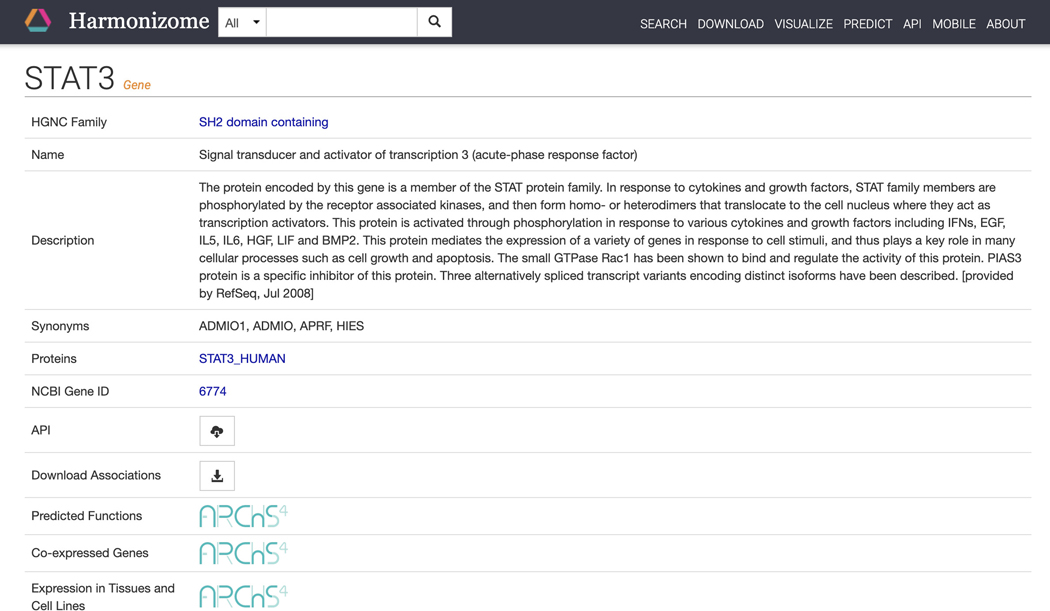
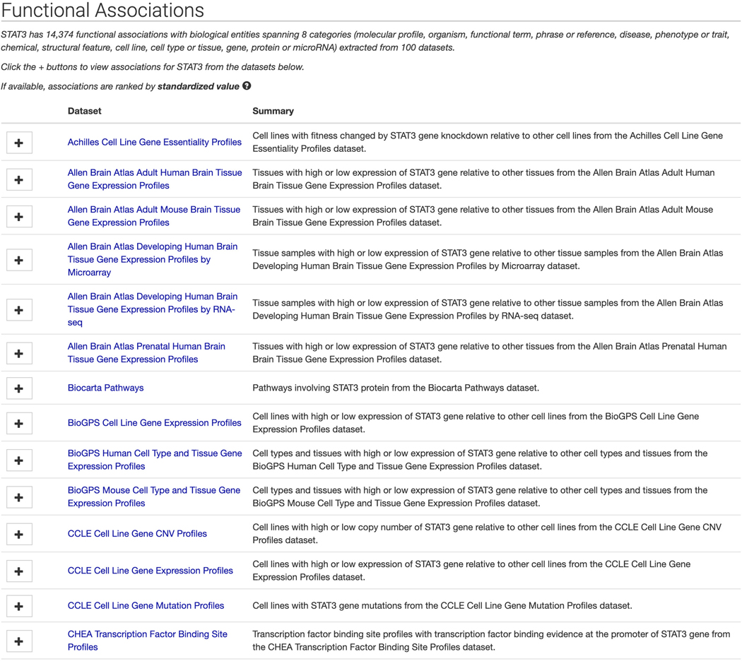
Click on the STAT3 “gene” result to be redirected to a single gene landing page (Figure 16). The page includes identifying metadata for the gene, download links for accessing functional associations between STAT3 and other attributes, and links to other gene-related information from ARCHS4 (Lachmann et al., 2018). Additionally, a list of functional associations for STAT3 from the various processed datasets included in Harmonizome is available (Figure 17). Click the “+” button to view associations for STAT3 for any of the datasets.
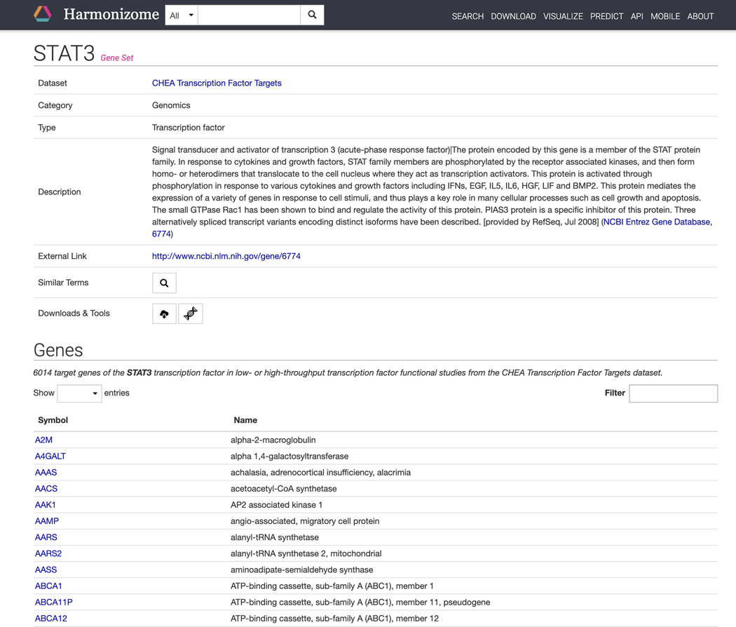
Click on any of the STAT3 “gene set” results. The gene set results page includes metadata for the STAT3 gene set, in this case the gene set includes all target genes of STAT3. All of the genes included in the gene set are found in the “Genes” section (Figure 18). Click on any of the gene symbols to be redirected to a single gene landing page.

Figure 14. — The Harmonizome homepage. The filter dropdown menu on the left selects between searching for genes, gene sets, and datasets.

Figure 15. — Search result page after querying “STAT3”. One gene page and 75 gene set pages match the query term “STAT3”.

Figure 16. — STAT3 single gene landing page that includes identifying metadata for the gene, download links for retrieving functional association data, and gene-related information from ARCHS4.

Figure 17. — Expandable lists of functional associations for STAT3 from each dataset.

Figure 18. — STAT3 gene set page from CHEA Transcription Factor Targets dataset.

Download Page

1
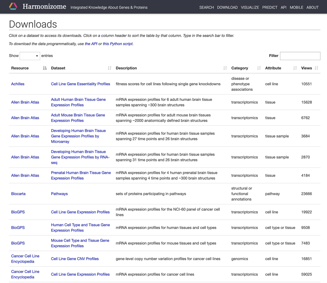
Click on the “Download” section on the navigation bar at the top of the page to be redirected to a table of all the datasets included in Harmonizome (Figure 19).
2
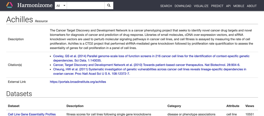
Click on “Achilles” in the resource column to be redirected to a page with identifying metadata for the resource and a list of all datasets derived from the resource (Figure 20).
3
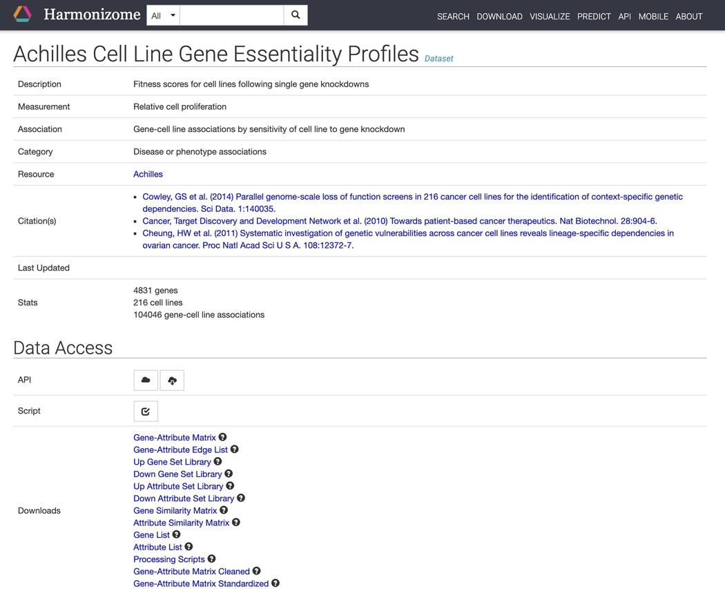
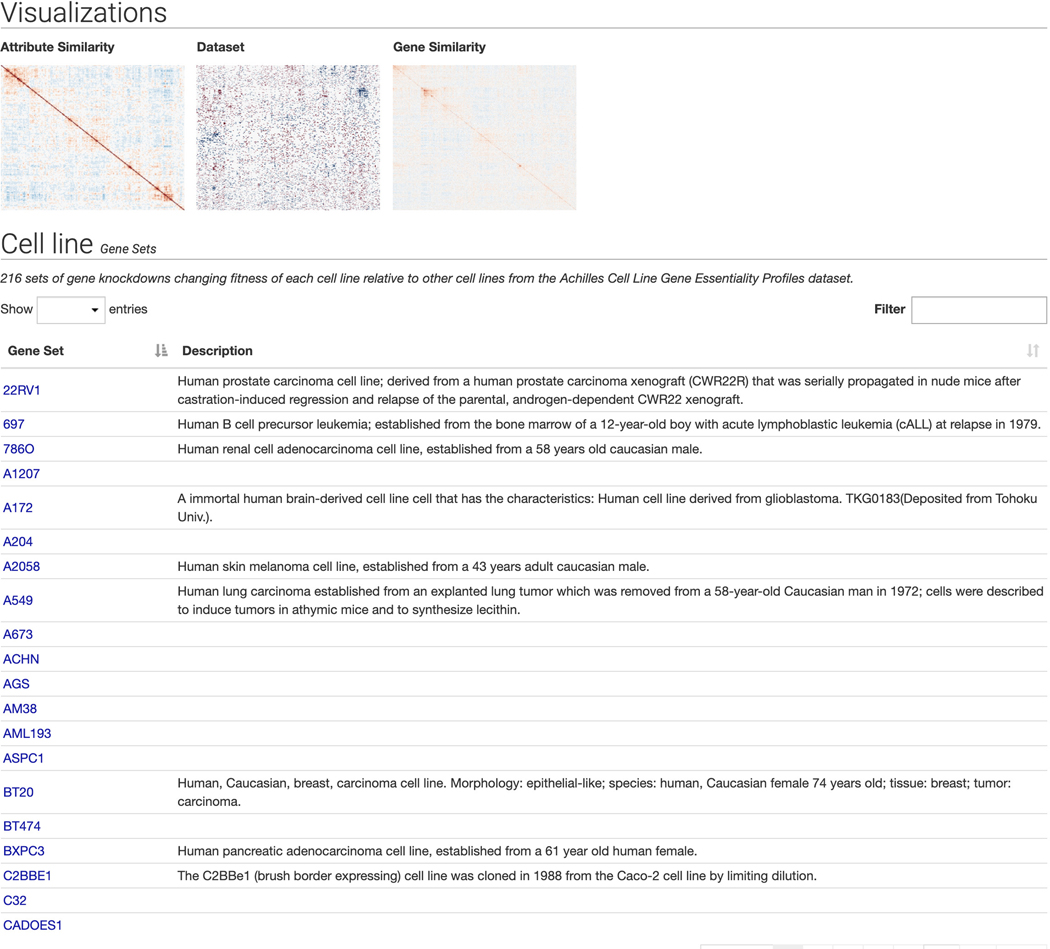
Click on “Cell Line Gene Essentiality Profiles” in the dataset column to be redirected to a page with identifying metadata for the dataset and links to downloadables contained within this dataset (Figure 21). Further down the page are links to visualizations of the dataset contents and a table of gene sets (Figure 22). Click on any of the gene set names to be redirected to a gene set specific page.

Figure 19. — Download page for datasets included in Harmonizome.

Figure 20. — Resource page for Achilles with identifying metadata for the Achilles resource.

Figure 21. — Dataset page for “Achilles Cell Line Gene Essentiality Profiles” with identifying metadata for the dataset, in addition to download links for files included in this dataset.

Figure 22. — Links to visualizations of the dataset contents and a table of gene sets. Click any of the gene sets to be redirected to a gene set specific page.

Visualize

4
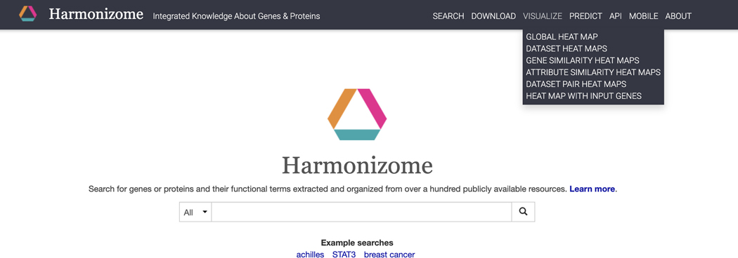
Click on the “Visualize” section on the navigation bar at the top of the page and a dropdown menu will appear (Figure 23).
5
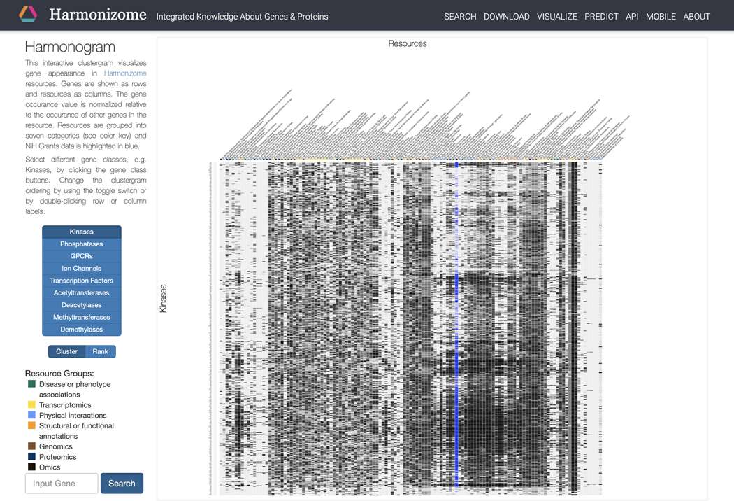
Click on “Global Heat Map” within the dropdown menu to be redirected to an interactive clustergram that visualizes the appearances of each gene in Harmonizome. Select different gene classes with the buttons on the left. Switch the ordering of the clustergram between “cluster” and “rank” by clicking the corresponding button (Figure 24).
6
Click on “Dataset Heat Maps” or “Gene Similarity Heat Maps” or “Attribute Similarity Heat Maps” within the dropdown menu to be redirected to a page with a dropdown menu of Harmonizome datasets. Open the dropdown menu and select any dataset to generate a hierarchically clustered heat map visualization of the dataset (Figure 25).
7
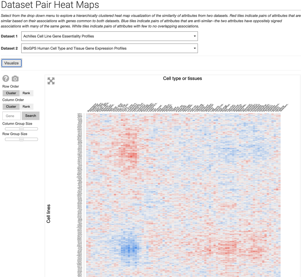
Click on “Dataset Pair Heat Maps” within the dropdown menu to be redirected to a page with a dropdown menu of Harmonizome datasets. Open the dropdown menu and select a dataset. A second dropdown menu will appear for selecting a second dataset to compare. Click visualize to generate a hierarchically clustered heat map visualization of the two datasets (Figure 26).
8
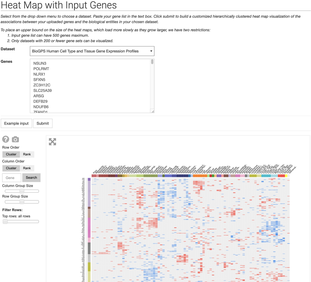
Click on “Heat Map with Input Genes” within the dropdown menu to be redirected to a page with a dropdown menu of Harmonizome datasets and a gene list text box. Click the “Example input” button to populate the fields with an example dataset and gene set. Click “Submit” to generate a hierarchically clustered heat map visualization of the associations between the uploaded genes and biological entities in the dataset (Figure 27).

Figure 23. — Dropdown menu of visualization page options.

Figure 24. — Global Heat Map visualization organized by gene families and resources. Switch between gene families using the buttons on the left. Switch between “Cluster” and “Rank” using the toggle on the left. Query a gene of interest using the search bar at the bottom left.

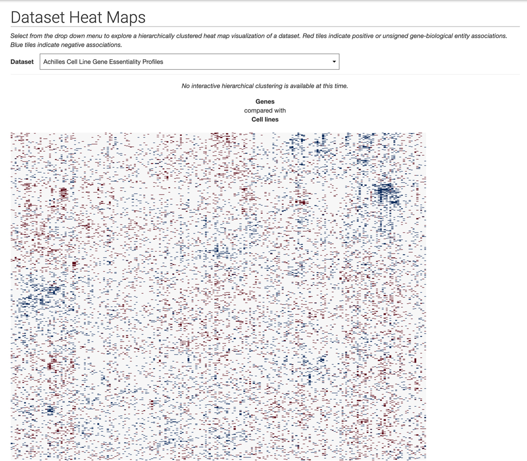
Figure 25. — Dataset Heat Maps page. Select a dataset from the dropdown menu and it will be visualized as a hierarchically clustered heat map.

Figure 26. — Dataset Pair Heat Maps page. Select two datasets to compare from the dropdown menus and a hierarchically clustered heat map will be generated.

Figure 27. — Heat Map with Input Genes page. Input a list of maximum 500 genes and select a dataset to build a hierarchically clustered heat map detailing associations between the input genes and biological entities in the dataset.

Predict

9
Click on the “Predict” section on the navigation bar at the top of the page and a dropdown menu will appear (Figure 28). Click “Intro” within the dropdown menu.
10
The intro page contains information about how machine learning studies were devised using the Harmonizome datasets. A table with four separate case studies: “Ion Channel Predictions”, “Mouse Phenotype Predictions”, “GPCR-Ligand Interaction Predictions”, “Kinase-Substrate Interaction Predictions” contains links to view and download tables of predicted associations (Figure 29).

Figure 28. — Dropdown menu of “Predict” options.

Figure 29. — Machine learning case studies page with details about the case studies were performed. Click on the corresponding buttons to view the tables for each study or download the table of predicted associations.

Using the Harmonizome API

11
These are the entity types supported by the Harmonizome API:

DATASET, GENE, GENE_SET, ATTRIBUTE, GENE_FAMILY, NAMING_AUTHORITY, PROTEIN, RESOURCE

Open a new or existing Python code file. Import the required Harmonizome API Python module at the top of the file:

from harmonizomeapi import Harmonizome, Entity

The Harmonizome object includes several methods to read, parse, and download data from the Harmonizome API. The Harmonizome object includes .get().next() and .download() methods. For example, to display the datasets available in Harmonizome run the following code block:

entity_list = Harmonizome.get(Entity.DATASET)
more = Harmonizome.next(entity_list)

In order to minimize database queries and request times, the Harmonizome API uses a technique called “cursoring” to paginate large result sets. Therefore, the first line in the above code block returns the first 100 datasets, whereas the second line continues from where the previous entity list left off and retrieves the subsequent 14 datasets that are available in Harmonizome. The Harmonizome.get()and Harmonizome.next() methods can be used for all entity types supported by the Harmonizome API.

12
To download datasets available in Harmonizome to a local directory use the Harmonizome.download() generator function. Alternatively Harmonizome.download_df() can be used to download files and load them in directly as sparse (with an added sparse=True argument) or dense Pandas DataFrames (assumed). The function takes a list of datasets and downloadables as arguments. Leaving the datasets argument empty will download all datasets by default. Leaving the what argument empty will download all downloadables for each dataset by default. In the example code below, the “gene_attribute_matrix.txt.gz” downloadable from the “CTD Gene-Chemical Interactions” dataset is downloaded, decompressed, and saved to a local directory named after the dataset if it hasn’t already been processed:

dl, = Harmonizome.download(datasets=[‘CTD Gene-Chemical Interactions’],
what=[‘gene_attribute_matrix.txt.gz’])

More information regarding the Harmonizome API is available at https://maayanlab.cloud/Harmonizome/documentation.

Basic Protocol 3: The ARCHS4 Resource

ARCHS4 (Lachmann et al., 2018) is a web resource that provides access to published RNA-seq gene and transcript level data from human and mouse experiments. FASTQ files from RNA-seq experiments deposited in the Gene Expression Omnibus (GEO) were aligned using a cloud-based infrastructure. The ARCHS4 web interface facilitates the exploration of the processed data through querying tools, interactive visualizations, and single gene landing pages that provide average expression of a specific gene across cell lines and tissues, top co-expressed genes, and predicted biological functions and protein–protein interactions for each gene based on prior knowledge combined with co-expression.

Necessary Resources

Hardware

Desktop or a laptop computer, or a mobile device, with a fast Internet connection

Software

An up-to-date web browser such as Google Chrome (https://www.google.com/chrome/), Mozilla Firefox (https://www.mozilla.org/en-US/firefox/), Apple Safari (https://www.apple.com/safari/), or Microsoft Edge (https://www.microsoft.com/en-us/edge).
Most updated version of R (https://www.r-project.org/); R Studio (https://www.rstudio.com/); rhdf5 library (https://www.bioconductor.org/packages/release/bioc/html/rhdf5.html)

Protocol steps and annotations

Metadata Search

1
Navigate to the ARCHS4 web application (https://maayanlab.cloud/archs4/).
2
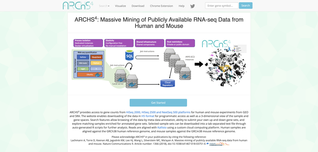
Click the “Get Started” button on the homepage to proceed to the data search and visualization page (Figure 30).
3
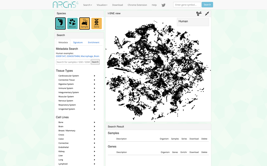
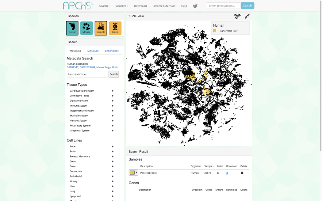
The data search and visualization page by default shows an interactive 3D t-SNE scatter plot of all the human gene expression samples found in ARCHS4 (Figure 31). The metadata search field on the left enables querying of specific terms which will be highlighted in the 3D scatter plot. Searching for the term “Pancreatic Islet” and then clicking on the search button results in the highlighting of the relevant samples. The samples that are related to the search term cluster in the scatter plot because the samples contain similar expression profiles (Figure 32).
4
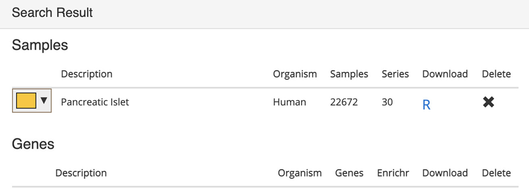
Any submitted search term will be found in its corresponding section within the “Search Result” table below the interactive t-SNE scatter plot visualization. The table contains metadata regarding the organism, number of samples, number of series, as well as a button to download an R script that can be used to retrieve the identified sample files. An X button is also available to delete the query (Figure 33).

Figure 31. — Data visualization and search page that includes a 3D interactable scatter plot of gene expression data.

Figure 32. — 3D scatter plot of human gene expression data that includes the term “Pancreatic islet”.

Figure 33. — Search results table with Pancreatic islet samples listed in their respective section with metadata and options to download an R script to process the samples or delete the query.

Signature Search

5
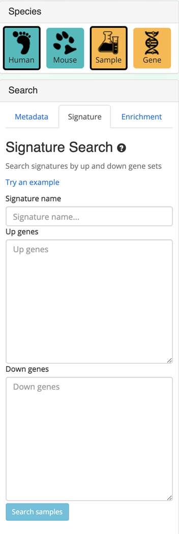
Switching to the signature search functionality can be done by clicking on the corresponding tab within the “Search” field on the left (Figure 34). The signature search uses a set of highly and lowly expressed genes from each sample to identify matching samples to the given input.
6
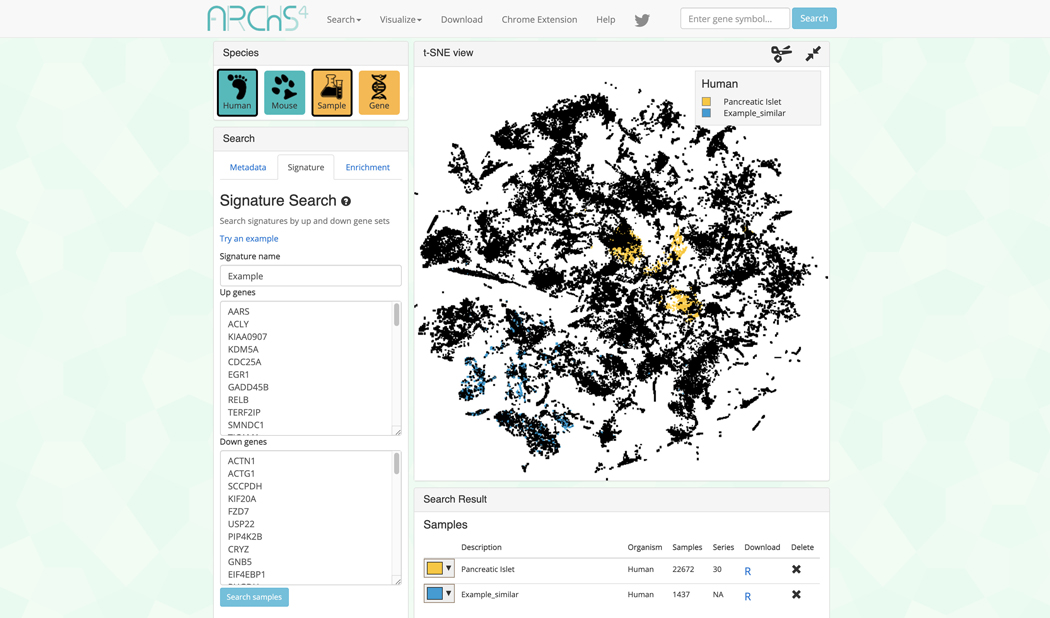
Query the example up and down gene sets by clicking “Try an example”. The corresponding samples are highlighted within the scatter plot and are added to the “Search Result” table (Figure 35). Note that the previous query of “Pancreatic Islet” is still visualized within the scatter plot and listed in the “Search Result” table.

Figure 34. — Signature search field that allows for querying of up and downregulated genes to identify samples that match the input.

Figure 35. — Example query from the signature search visualized in the 3D scatter plot. The identified samples are added to the “Search Result” table.

Enrichment Analysis

7
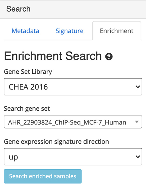
Switch to the enrichment search by clicking on the corresponding tab within the “Search” field on the left (Figure 36). The enrichment search highlights samples that are enriched in gene sets from eight gene set libraries. Select the gene set library, gene set of interest within the selected library, and a signature direction.
8
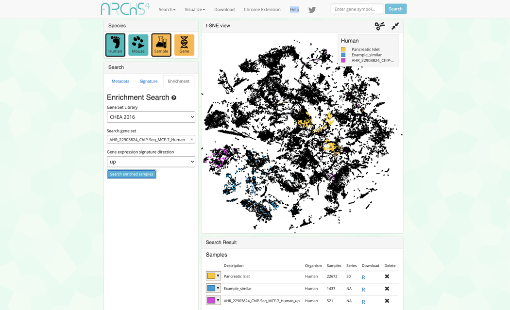
Query the example by clicking “Search enriched samples”. The corresponding samples are highlighted within the scatter plot and added to the “Search Result” table along with the previous queries (Figure 37).

Figure 36. — Enrichment search field that allows for selection gene set library, gene set within the library, and choice of upregulated or downregulated signatures.

Figure 37. — Example query from the enrichment search visualized in the 3D scatter plot. The identified samples are added to the “Search Result” table.

Gene-Centric Visualization

9
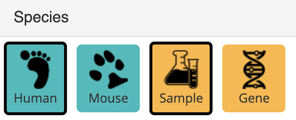
Switch to gene-centric searches by clicking on the orange button under the “Species” field in the upper left. Use this field to also switch between human and mouse samples by clicking the corresponding teal button (Figure 38).
10
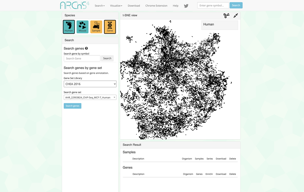
The page will now contain an interactive t-SNE scatter plot where each point represents a gene instead of a sample (Figure 39).
11
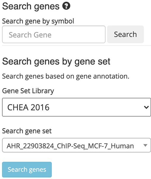
Choose a gene set library and a gene set within the “Search” field on the left (Figure 40). Query the default options by clicking “Search genes”.
12
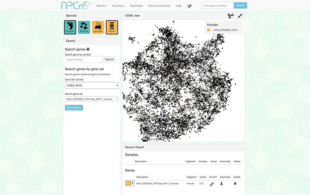
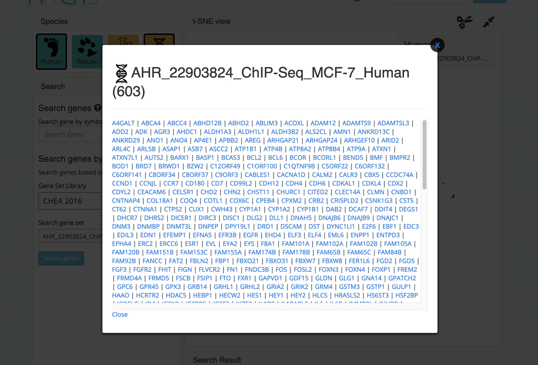
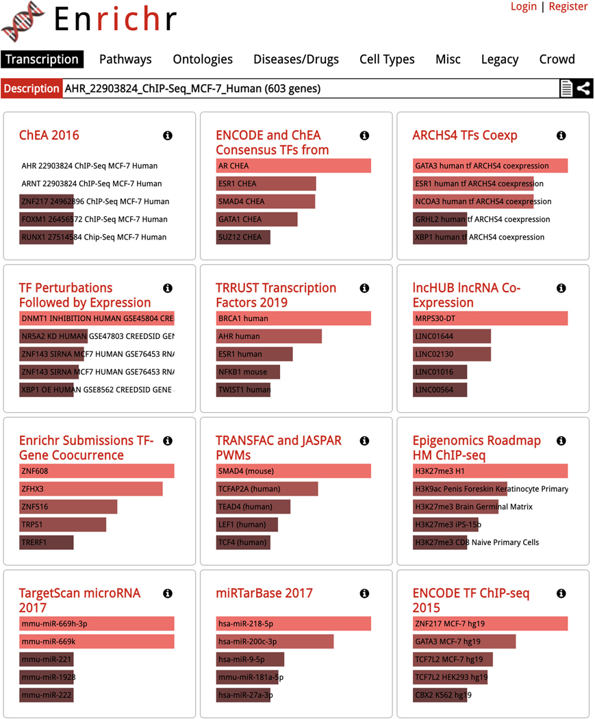
The corresponding samples are highlighted within the scatter plot and added to the “Search Result” table under the “Genes” section (Figure 41). The table includes the number of genes included in the queried gene set which can be clicked to view the gene symbols in the gene set (Figure 42). Additionally, the gene set can be submitted to Enrichr (Kuleshov et al., 2016) for gene set enrichment analysis by clicking on the Enrichr icon within the table (Figure 43).

Figure 38. — Selection buttons for switching between human and mouse samples, as well as buttons for switching between sample queries and single gene queries.

Figure 39. — Scatter plot of single genes instead of samples where the distance between genes quantifies similarity of their expression profiles across all samples in ARCHS4.

Figure 40. — Search genes by gene set” field where a gene set library and gene set within the library are selected to be queried.

Figure 41. — Genes from the selected gene set library and gene set are displayed on the scatter plot. The genes are added to their respective section in the “Search Result” table.

Figure 42. — Clicking on the number of genes in the “Search Result” table displays the genes included in the queried gene set.

Figure 43. — Clicking on the Enrichr icon in the “Search Results” table displays gene set enrichment analysis results for the genes from the queried gene set.

Gene Search

13
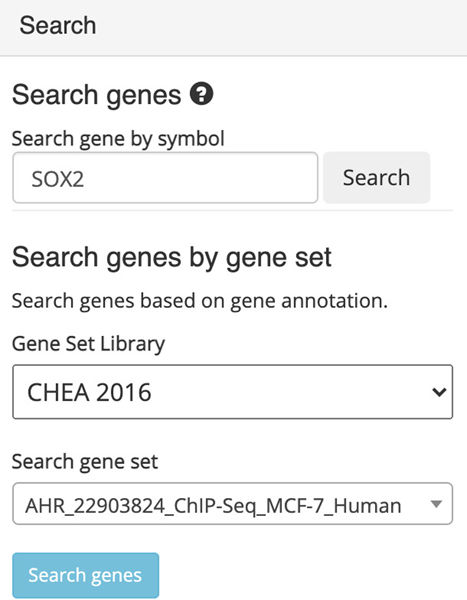
Single genes can be queried using the autocomplete field within the “Search” field on the left. Input a gene of interest, for example SOX2, and click the search button (Figure 44).
14
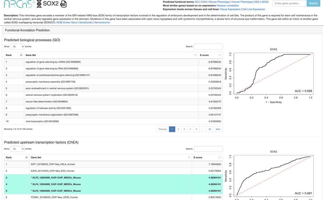
A single gene page is generated for SOX2 (Figure 45). The top of the page includes a description of the gene and links to other resources with identifying metadata for the gene. The “Functional Annotation Prediction” section contains ROC curves and tables of gene sets from six distinct gene set libraries SOX2 is predicted to be a member of based on co-expression. Known associations are marked in teal.
15
The “Most similar genes based on co-expression” section contains a table of the top 100 genes that are most similar to SOX2 based on the Pearson correlation of their expression across all ARCHS4 samples (Figure 46). The most correlated genes from the table can be submitted to Enrichr by clicking the corresponding link in the top right.
16
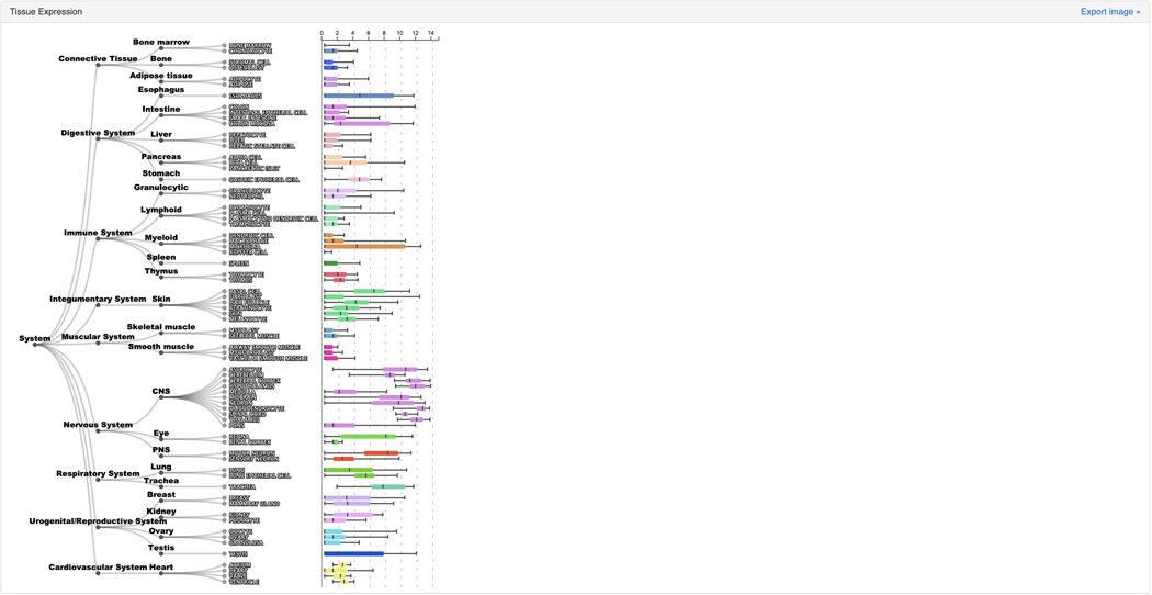
The “Tissue Expression” section contains a dendrogram of tissue types divided into organs and cell types. The average expression of SOX2 within a specific tissue or a cell type context is visualized as a collection of box plots (Figure 47).
17
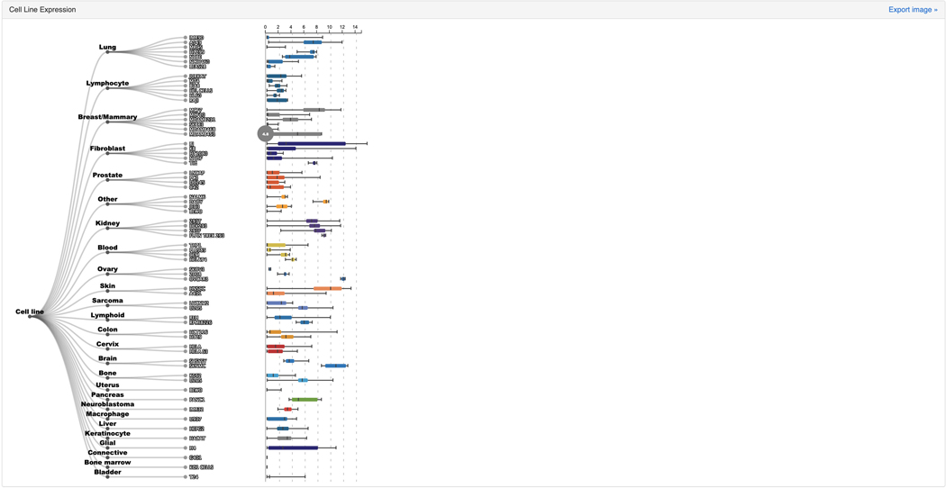
The “Cell Line Expression” section contains a dendrogram of various cell lines organized by the tissue of origin. The plot visualizes the average expression of SOX2 across the cell lines based on data from ARCHS4 (Figure 48).

Figure 44. — “Search genes” field populated with the gene symbol “SOX2”.

Figure 45. — Single gene page for SOX2 with identifying metadata at the top of the page. Additionally, tables of predicted functions from various gene set libraries are depicted along with ROC curves to quantify the ability to predict gene sets that SOX2 is a known member of from co-expression data.

Figure 46. — Table of the top 100 genes most similar to SOX2 based on co-expression. The genes can be submitted to Enrichr by clicking the “Upload to Enrichr” button.

Figure 47. — Tissue expression atlas for SOX2 that quantifies the expression of SOX2 in various tissue types.

Figure 48. — Cell line expression atlas for SOX2 that quantifies the expression of SOX2 in various cell lines.

Downloading Gene Expression Data from ARCHS4

18
As described in previous steps, after submitting a search within the data search and visualization page, the “Search Results” table includes a download link to an R script that can be used to retrieve the selected samples. Click the download icon to download the script.
19
Open R Studio and copy and paste the R script from the downloaded R file into R Studio.

Ensure that the “rhdf5” library is installed. Open the console in R Studio and input the following:

if (!requireNamespace(“BiocManager”, quietly = TRUE))
    install.packages(“BiocManager”)
BiocManager::install(“rhdf5”)

21
Now run the R script downloaded from ARCHS4 to produce an expression matrix for the selected samples that were returned from the search. The expression matrix can be used for further analysis, for example, it can be used to compute the average expression of a gene in a specific disease, cell line, or tissue contexts.

Basic Protocol 4: Making predictions about gene function with PrismExp

PrismEXP is an Appyter (Clarke et al., 2021; Lachmann et al., 2021) that employs machine learning to predict gene function using gene-gene mRNA co-expression correlations from mRNA-sequencing (RNA-seq) data sourced from ARCHS4, a database composed of human and mouse RNA-seq sample gene counts from GEO (Lachmann et al., 2018). The difference between gene function predictions made by PrismExp and the gene function prediction available from the ARCHS4 website is that the ARCHS4 data is divided first into clusters and then gene-gene correlations are computed for each cluster. 51 correlation matrices are precomputed and stored in the cloud. At runtime, the correlation data is extracted from the cloud storage and a pretrained Random Forest model is applied on the correlation features to rank the level of association of a single gene to all gene sets from a user-specified gene set library.

Necessary Resources

Hardware

Desktop or a laptop computer, or a mobile device, with a fast Internet connection

Software

An up-to-date web browser such as Google Chrome (https://www.google.com/chrome/), Mozilla Firefox (https://www.mozilla.org/en-US/firefox/), Apple Safari (https://www.apple.com/safari/), or Microsoft Edge (https://www.microsoft.com/en-us/edge).

Protocol steps and annotations

Navigating the Input Form

1
Navigate to the PrismEXP Appyter (https://appyters.maayanlab.cloud/PrismEXP/).
2
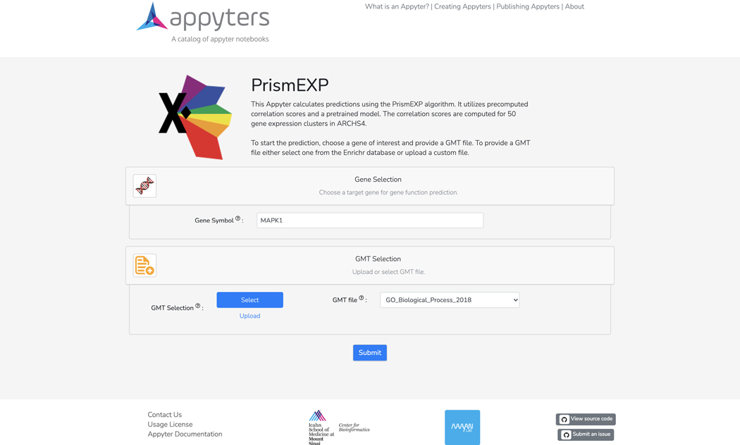
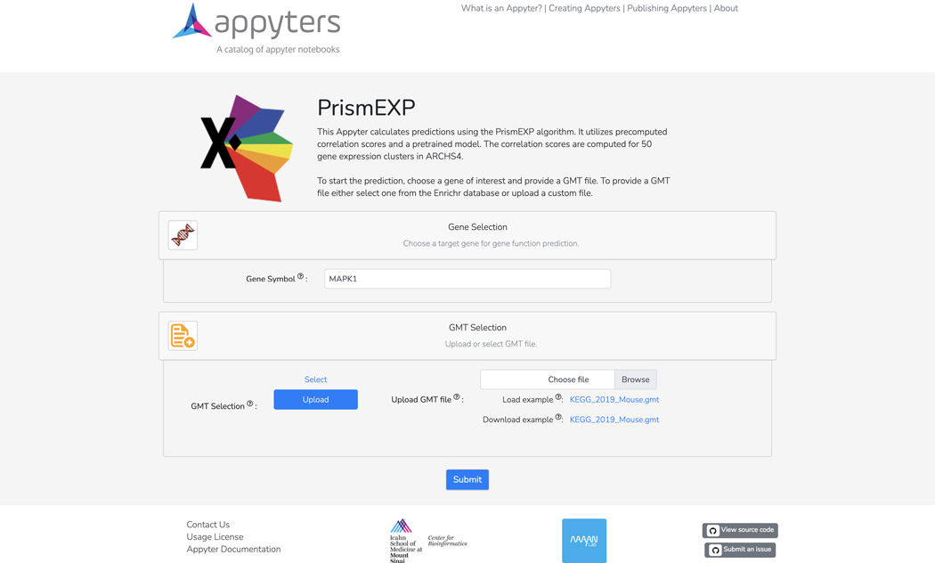
The Appyter input form includes a “Gene Selection” section with a field for inputting a gene symbol of interest for which novel functions will be predicted. Additionally, the “GMT Selection” section includes a field for selecting a GMT file from which predictions will be made (Figure 49). Click the “Upload” button within the “GMT Selection” section to upload a custom GMT file (Figure 50).
3
Click submit on the Appyter input form and a Jupyter Notebook with the input parameters will be launched in the cloud.

Figure 49. — PrismEXP Appyter input form where the user is prompted to input a gene symbol of interest and specify a gene set library (in GMT format) to make predictions from.

Figure 50. — Alternative input form option for uploading a custom GMT file.

Gene Function Predictions

4
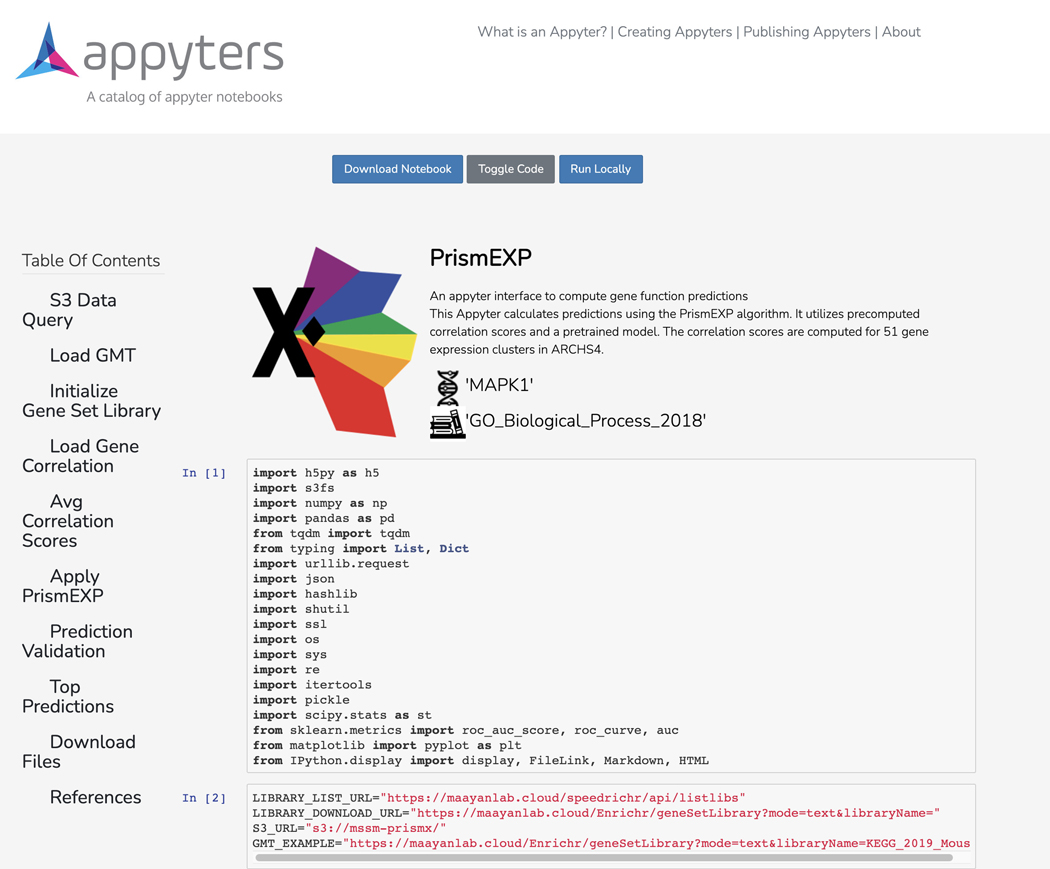
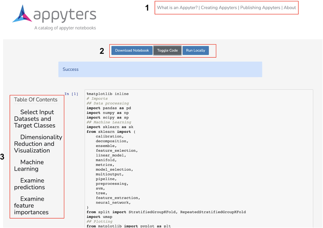
A Jupyter Notebook will begin executing in the cloud once the input form is submitted. The notebook includes an option to download the notebook, toggle displaying the code, and running the notebook locally. Additionally, a table of contents exists with clickable elements that link to specific sections within the notebook (Figure 51).
5
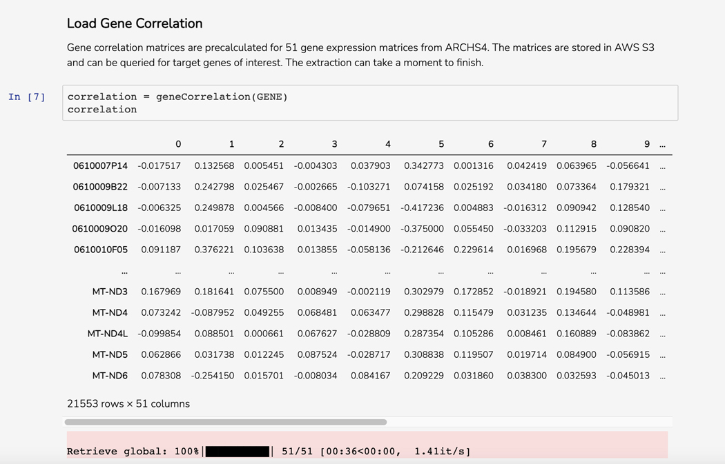
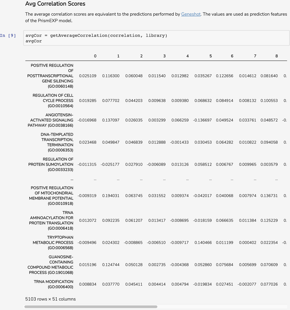
Scroll down to the “Load Gene Correlation” section. The Dataframe displays genes that correlate with your query gene in 51 pre-computed correlation matrices from ARCHS4 (Figure 52).
6
Scroll down to the “Avg Correlation Scores’’ section. This Dataframe displays computed correlation scores to each of the gene set terms from the GMT file based on co-expression values between the query gene and each of the genes included in the gene set (Figure 53).
7
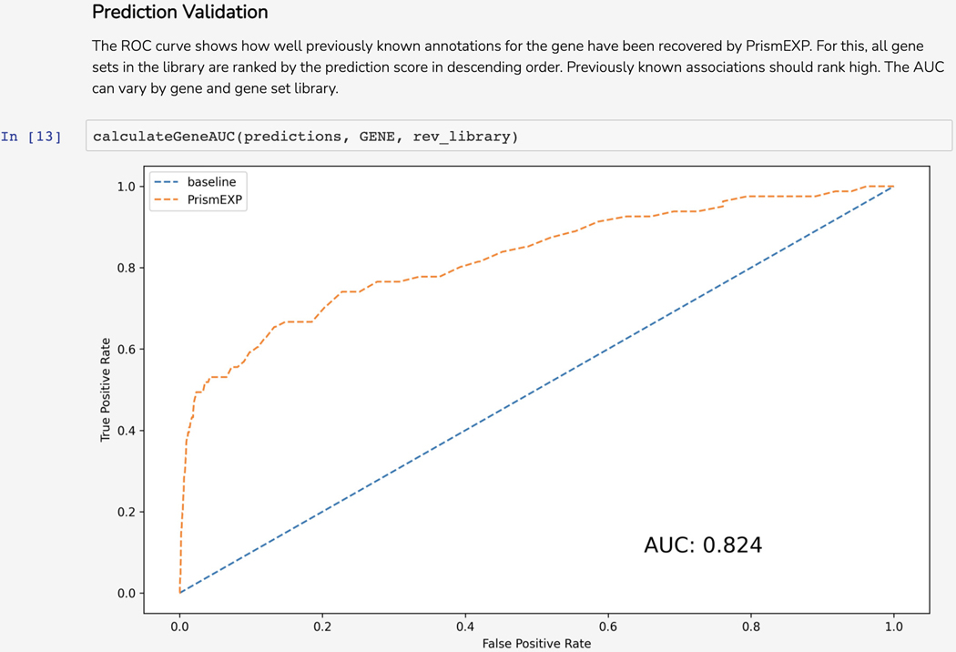
The average correlation score matrices are used as the input features for the PrismEXP model. Scroll down to the “Prediction Validation” section. The ROC curve displayed in this section characterizes how well the known annotations for this gene were recovered by the PrismEXP model (Figure 54).
8
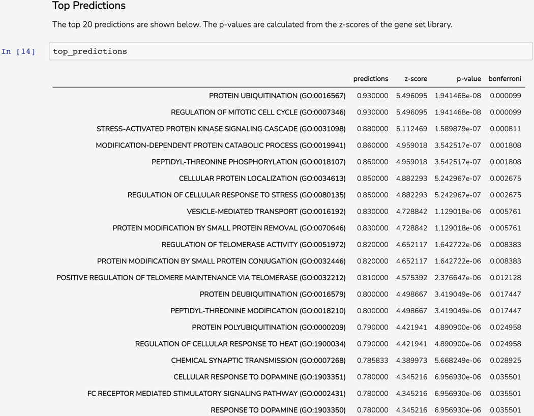
Scroll down to the “Top Predictions’’ section. The Dataframe displays the top 20 gene set terms that the query gene is predicted to be associated with. The table displays the prediction score from the model, z-score, p-value, and Bonferroni corrected p-value (Figure 55).
9
Scroll down to the “Download Files” section. Click on the appropriate link to download the prediction table or ROC curve in .pdf or .png format (Figure 56).

Figure 51. — The launched Appyter notebook with options to download the notebook, toggle the code, and instructions for running the Appyter locally. Additionally, a table of contents on the left allows for easy traversal between sections of the notebook.

Figure 52. — Dataframe of 51 correlation matrices, each displaying correlation values between the query gene and other mouse genes.

Figure 53. — Dataframe of average correlations between each gene set from the specified gene set library and the query gene from the previous 51 correlation matrices.

Figure 54. — ROC curve that quantifies the ability of the PrismEXP model to retrieve previously known associations between gene set annotations and the query gene.

Figure 55. — Table of top predicted associations for the query gene.

Figure 56. — Download links to prediction table and ROC curve image.

Basic Protocol 5: Using Geneshot to illuminate knowledge about under-studied targets

Geneshot is a search engine for querying biomedical terms to retrieve lists of genes most associated with the term from PubMed ID (PMID) co-mentions (Lachmann et al., 2019). To convert search terms to genes, Geneshot uses one of two resources: GeneRIF and AutoRIF. Both GeneRIF and AutoRIF are text files documenting gene-PubMed ID associations. These associations are used to rank genes for a query term based on the number of co-mentions. Geneshot further prioritizes other related genes based on co-occurrence and co-expression matrices with the genes associated with the term from the literature. Additionally, Geneshot includes a gene function prediction feature that prioritizes novel gene set membership for a query gene based on co-occurrence or co-expression.

Necessary Resources

Hardware

Desktop or a laptop computer, or a mobile device, with a fast Internet connection

Software

An up-to-date web browser such as Google Chrome (https://www.google.com/chrome/), Mozilla Firefox (https://www.mozilla.org/en-US/firefox/), Apple Safari (https://www.apple.com/safari/), or Microsoft Edge (https://www.microsoft.com/en-us/edge).
Text editor or development environment of choice, such as Visual Studio (https://visualstudio.microsoft.com/vs/); most updated version of Python (https://www.python.org/downloads/); Python requests library (https://requests.readthedocs.io/en/master/user/install/)

Protocol steps and annotations

PubMed Query

1
Navigate to the Geneshot homepage (https://maayanlab.cloud/geneshot/).
2
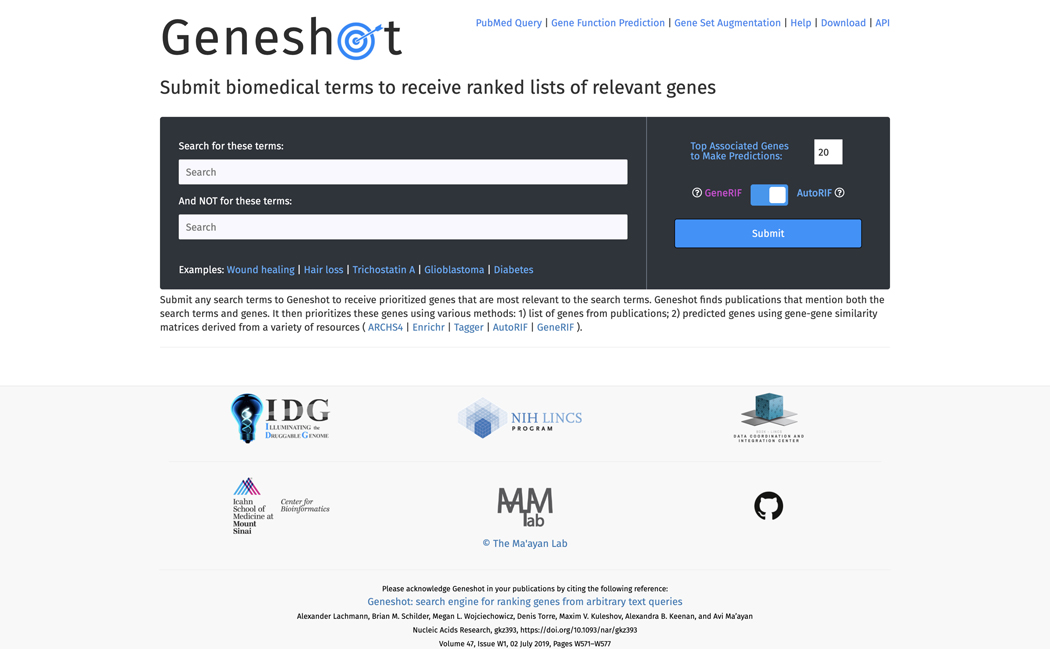
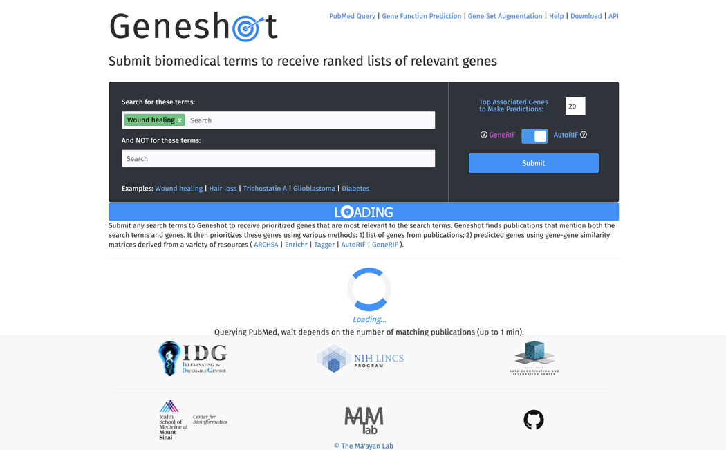
The PubMed Query page includes an input form for submitting search terms (Figure 57). The top search bar is for terms that the search should include, whereas the lower search bar is for terms that should be omitted from the search. Toggle the size of the gene set that will be used to make further predictions with the “Top Associated Genes to Make Predictions” filter. Use the toggle bar to switch between AutoRIF and GeneRIF (Maglott et al., 2011) as the underlying databases for gene-PMID associations. Click “Wound Healing” in the example section of the input form to launch a search (Figure 58).
3
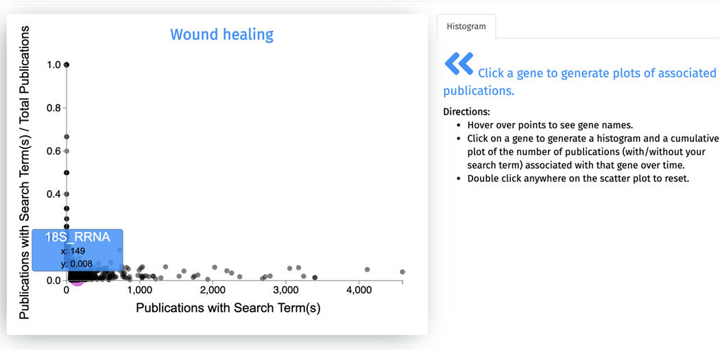
The first output from the search is a scatter plot of all genes associated with “wound healing” (Figure 59). The x-axis of the scatter plot displays the counts of Publications with Search Term, and the y-axis shows the fraction of Publications with Search Term / Total Publications. Hover over any point on this plot to display the gene name and its corresponding X and Y values.
4
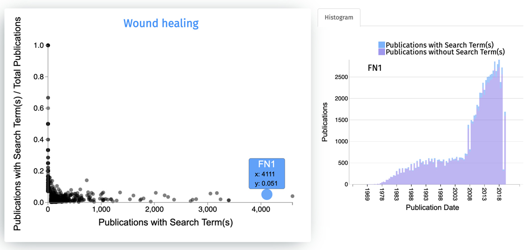
Clicking on any of the points in the scatter plot generates a histogram displaying the association of the gene with the search terms based on literature co-mentions over time (Figure 60). The number of publications for the selected gene that do not match the search term is displayed as pink bars, while the number of publications matching the search term and the gene is displayed as blue bars.
5
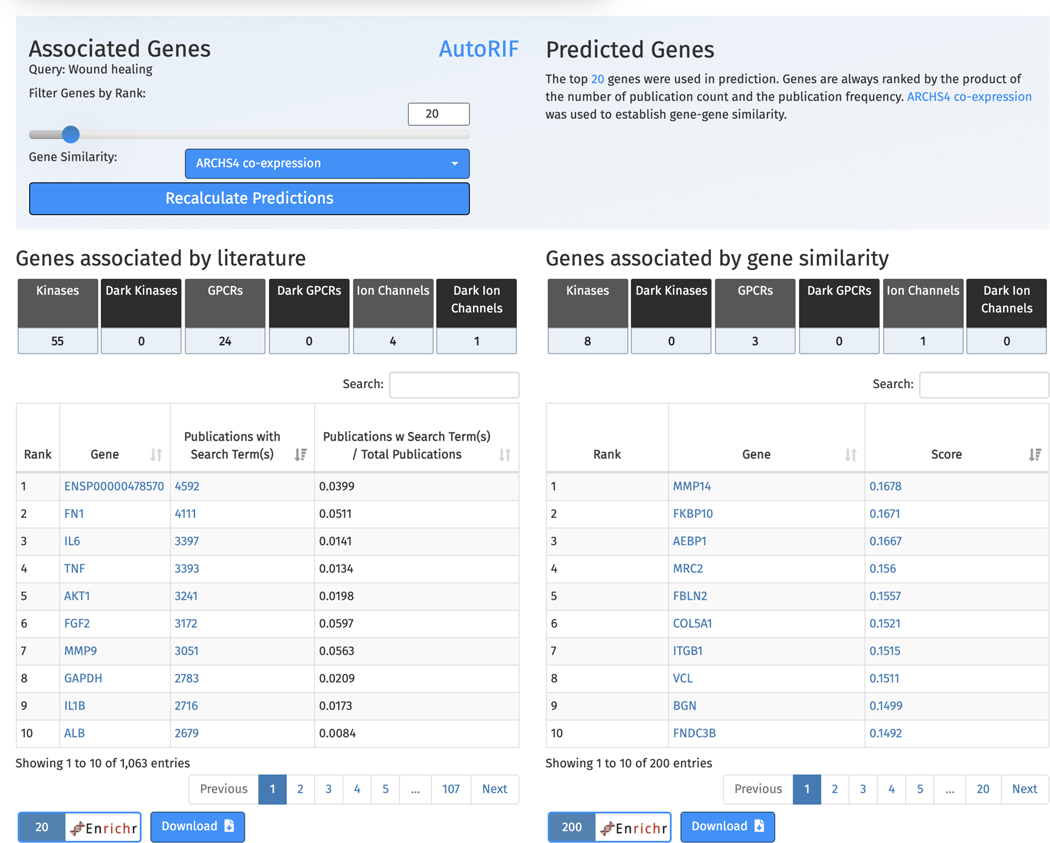
Scroll down to view the tables of associated genes and predicted genes (Figure 61). The left table includes the top genes associated with “wound healing” ranked by number of PubMed ID co-mentions. The right table shows the top 200 genes predicted to be associated with “wound healing” based on co-expression with the top 20 genes from the associated table. Each of the tables include a row of buttons that, when clicked, filter the genes from each table into a specific gene family. Additionally, the genes from each table can be submitted to Enrichr for gene set enrichment analysis, and each table itself can be downloaded.
6
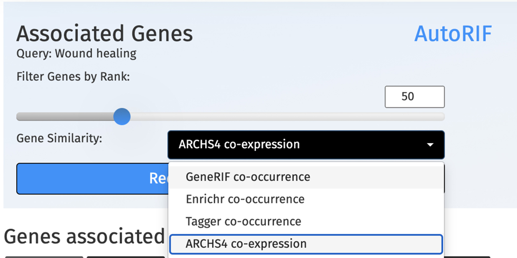
To recalculate the predictions, use the drop-down menu above the associated table to select a new gene-gene similarity matrix and increase or decrease the associated gene set size using the scroll bar. Click the “Recalculate Predictions” button to update the prediction table (Figure 62).

Figure 57. — Geneshot homepage. The search bars allow for querying terms to be included and omitted from the search. Additional options exist for toggling between GeneRIF and AutoRIF and adjusting the gene set size for making predictions.

Figure 58. — Submitted search form populated with the term “Wound healing”.

Figure 59. — Scatter plot of all genes associated with “wound healing”. Each point represents a gene and interacting with any point reveals the gene name, X-axis value, and Y-axis value.

Figure 60. — Clicking on any of the points in the scatter plot generates a histogram of associations between the gene and “wound healing” over time. The blue bars represent publications mentioning the gene and search term, whereas purple bars represent publications mentioning just the gene.

Figure 61. — Table of top genes associated with “wound healing” ranked by number of publications that mention the gene and search term (left). Table of genes predicted to be associated with “wound healing” based on co-expression with the literature derived genes (right). Both tables can be downloaded and the genes from both tables can be submitted to Enrichr for gene set enrichment analysis.

Figure 62. — The predicted gene table from the “wound healing” search can be recalculated by selecting a different gene-gene similarity matrix for predictions and changing the gene set size derived from the associated gene table.

Gene Function Predictions

7
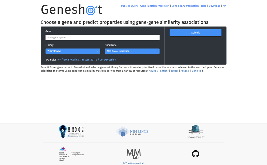
Navigate to the Gene Function Prediction page by clicking the corresponding link within the navigation bar at the top of the page. This page includes an input form for selecting a gene of interest, Enrichr gene set library from which gene functions will be sourced from, and a gene-gene similarity matrix from which predictions will be calculated (Figure 63). By using functional prediction by association, the input gene can be predicted to be a member of gene sets. Click the example to launch a query.
8
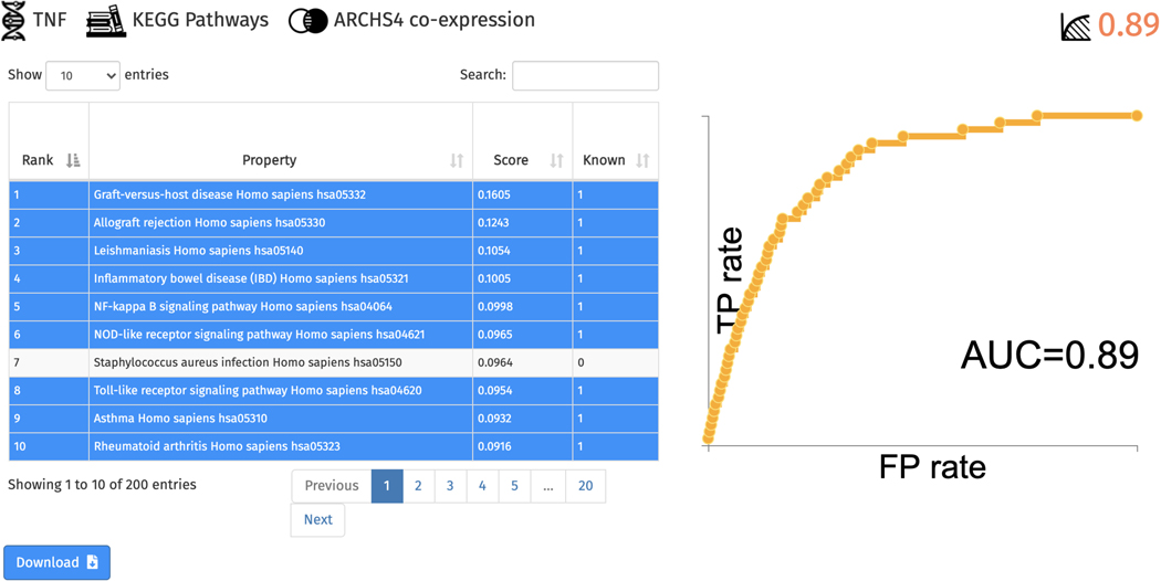
A table of the top predicted functions and ROC curve of prediction performance are generated (Figure 64). Known associations within the table are highlighted in blue, whereas previously unknown associations are not highlighted. The table is available for download.

Figure 63. — Gene function prediction page. The input form allows for the selection of a query gene, a gene set library from which gene sets with functional association terms will be retrieved, and a gene-gene similarity matrix from which predictions will be made.

Figure 64. — Table of top predicted associations for TNF from the KEGG Pathways gene set library. Known functions are highlighted in blue. The ROC curve quantifies the ability of the prediction method to retrieve functions that TNF is known to be associated with.

Gene Set Augmentation

9
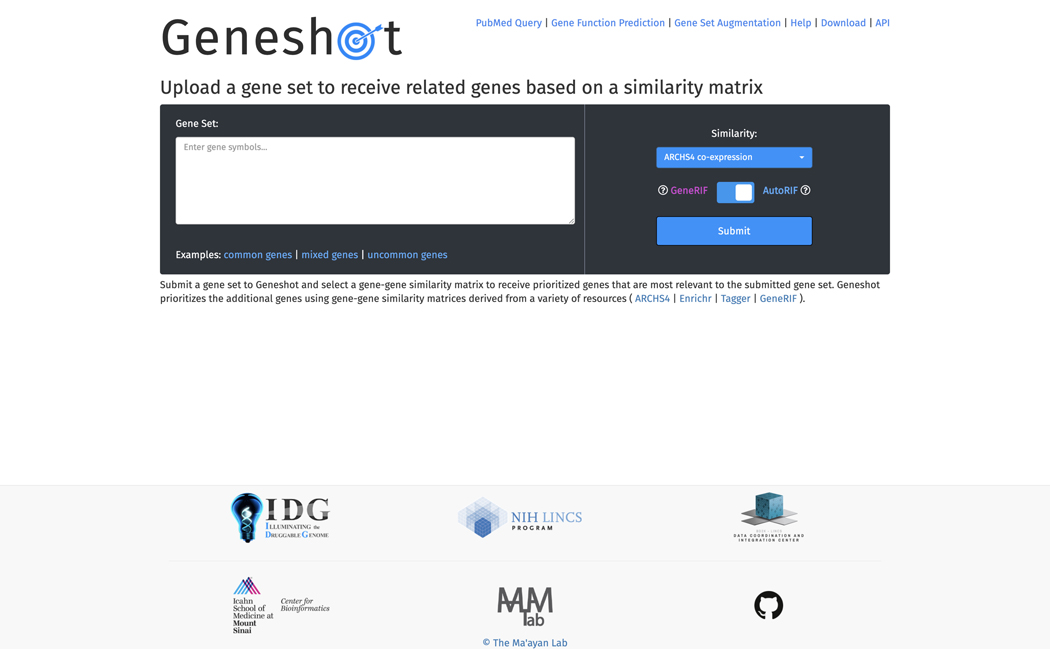
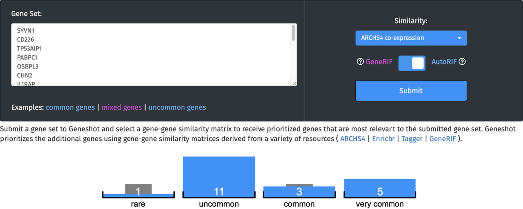
Navigate to the Gene Set Augmentation page by clicking the corresponding link within the navigation bar at the top of the page. The input form on this page includes a text box for pasting a gene set for augmentation, a drop-down menu of gene-gene similarity matrices from which predictions will be calculated, and a toggle bar for switching between GeneRIF and AutoRIF for retrieving publication counts for each gene (Figure 65).
10
Click on the “mixed genes” example to submit a query. The input genes are first sorted into quantiles based on their novelty in the literature (Figure 66).
11
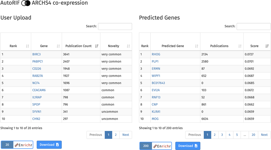
Scroll to the bottom of the page where there is a table with the submitted genes on the left, and a table of genes predicted to be associated with the input genes based on the selected gene-gene similarity matrix, in this case ARCHS4 co-expression, on the right (Figure 67). The “user upload” table ranks the genes by the amount of PubMed abstracts they are mentioned in, along with their novelty. The predicted genes table ranks genes by their similarity score with the input gene set. Genes from both tables can be submitted to Enrichr for gene set enrichment analysis and each table can be downloaded.

Figure 65. — Gene set augmentation page. The text box accepts a list of gene symbols that will be used as an unweighted gene set to predict related genes based on the selected gene-gene similarity matrix. The source of gene publication data can be changed with a toggle bar between GeneRIF and AutoRIF.

Figure 66. — The “mixed genes” example query with the quantile counts for each of the queried genes.

Figure 67. — Table of queried genes, their publication counts, and novelty (left). Table of top 200 genes predicted to be associated with the query gene set, gene publication counts, and similarity score with the query gene set (right). Each table can be downloaded and the genes from each table can be sent to Enrichr for gene set enrichment analysis.

Geneshot API Example

12
Open a new or existing Python code file. Import the JSON and requests libraries at the top of the file as follows.
```
import json
import requests
```
13
Call the requests.post method to send a POST request to the URL. The payload variable contains the parameters that are sent to the API endpoint specified in GENESHOT_URL. In this case the endpoint is /search and the parameters are rif, which specifies whether AutoRIF or GeneRIF is used as the association file, and term, which specifies the query term for the search.
```
GENESHOT_URL = ‘https://maayanlab.cloud/geneshot/api/search’
payload = {“rif”: “generif”, “term”: “hair loss”}
```
```
response = requests.post(GENESHOT_URL, json=payload)
```
```
data = json.loads(response.text)
print(data)
```
14
Use the json.loads method to view the response as a JSON object containing all genes related to the query term.

{
 “PubMedID_count”: 34412,
 “gene_count”: {
   “ABCC6P2”: [
    1,
    0.25
  ],
  “ABI3”: [
   2,
   0.125
  ],
  ...
  },
  “query_time”: 1.121943712234497,
  “return_size”: 298,
  “search_term”: “hair loss”
}

For more information on using the various Geneshot API endpoints, please refer to the API documentation (https://maayanlab.cloud/geneshot/api.html).

Basic Protocol 6: Exploring understudied targets with TIN-X

TIN-X (Target Importance and Novelty eXplorer) (Cannon et al., 2017), is an informatics workflow, REST API, and web application used to identify, visualize, and explore protein-disease associations. TIN-X is based on text mining data processed from scientific literature. The TIN-X visualizations plot information for protein-disease associations along two axes, specifically “novelty” and “importance.” Briefly, Novelty is used to estimate the scarcity of publications about a protein target, whereas Importance estimates the strength of the association between that protein and a specific disease.

Necessary Resources

Hardware

Desktop or a laptop computer, or a mobile device, with a fast Internet connection

Software

An up-to-date web browser such as Google Chrome (https://www.google.com/chrome/), Mozilla Firefox (https://www.mozilla.org/en-US/firefox/), Apple Safari (https://www.apple.com/safari/), or Microsoft Edge (https://www.microsoft.com/en-us/edge).

Protocol steps and annotations

Browse Diseases

1
Navigate to the TIN-X web app (https://www.newdrugtargets.org/).
2
The default TIN-X mode, “Browse Diseases”, (upper-left) starts with the Disease Ontology (Schriml et al., 2019), (DO). The DO hierarchy can then be navigated using the left panel (Figure 68). Given this hierarchical nature, a larger number of target-disease associations can be text-mined from biomedical literature for higher-level terms (e.g., N=13405 for “nervous system disease”), as opposed to child terms (e.g., N=9733 for “neurodegenerative disease”, N=4587 for “Synucleinopathy,” N=4587 for “Parkinson’s Disease”) or for leaf terms (e.g., N=227 for “Early Onset Parkinson’s Disease”).
3
Searching by disease name is also supported. Targets with stronger associations (higher Importance) are in the upper part of the plot, while targets with a higher number of publications (lower Novelty) are located on the left side of the plot. Points situated in the upper-right area of the plot (if any) are most likely to be of interest, as they are located at the Pareto frontier, i.e., targets for which a large number of published papers mentioning that target also mention the selected disease.
4
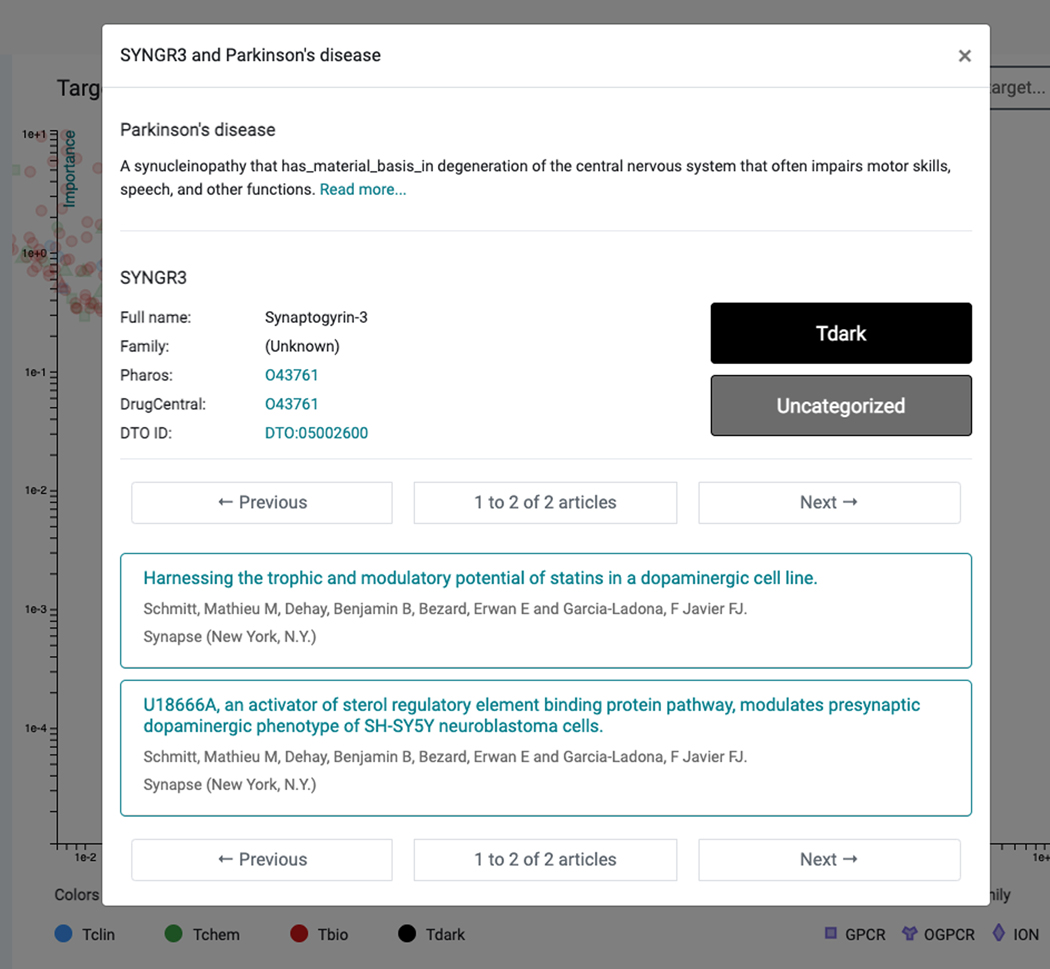
Targets are colored by Target Development Levels, and can be filtered as such (Tclin/Tchem/Tbio/Tdark). They can also be filtered by protein superfamily (e.g. kinases). Upon selecting a protein, links to both Pharos and DrugCentral are provided for that protein (Figure 69); selecting the titles allows the user to navigate through abstracts or to examine the document of interest in PubMed (additional clicks are required).
5
Once the desired level of granularity for diseases is reached, the user can examine target-disease associations, which are plotted along the Novelty-Importance axes in log-log format. To reach “Parkinson’s Disease”, one must click Disease of anatomical entity → Nervous System Disease → Neurodegenerative disease → Synucleinopathy → Parkinson’s Disease.
6
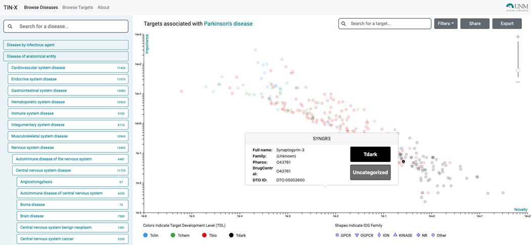
A highly-ranked gene associated with Parkinson’s Disease is “Synaptogyrin-3” (SYNGR3) and is classified as Tdark (Figure 69). While the exact function of SYNGR3 is unknown, there is recently published evidence that SYNGR3 encodes for a synaptic vesicle protein that interacts with a dopamine transporter(Egaña et al., 2009). The most novel association (lowest Importance) is for “Tripartite motif-containing protein 10” (TRIM10), which is supported by one genome-wide association study (Witoelar et al., 2017) focused on the overlap between Parkinson’s Disease and autoimmune diseases.
7
Both the “Browse Diseases” and the “Browse Targets” exploratory modes support an interactive way to manipulate the number of points displayed on the scatter plot. To change the number of plotted points, simply go to the top right side of the panel, where a vertical bar is placed between a “+” and a “-” sign. Sliding this bar up or down increases or decreases the number of visible points within the plot. By default, 300 or fewer points are plotted. Thresholds are defined by non-dominated solution (NDS) ranking, a.k.a. Pareto frontier, meaning that all hidden points are inferior to those visible in one or both variables.

Figure 68. — The TIN-X “Browse Disease” view (left side) with Parkinson’s Disease selected. Targets associated with Parkinson’s Disease (right side) are plotted on a log scale of Importance vs Novelty, with each data point colored according to its Target Development Level (TDL).

Figure 69. — Clicking a target point within the Parkinson’s Disease example, “Synaptogyrin-3” (SYNGR3) displays details including the full name and family of the target, Target Development Level (TDL), links to Pharos and DrugCentral, and, importantly, links to the associated two research articles (bottom).

Browse Targets

8
From the upper left menu, “Browse Targets” can be selected. The Drug Target Ontology (Lin et al., 2017) hierarchy becomes visible, and can be navigated from the left panel (Figure 70). For each protein, Diseases are plotted with log–log Importance–Novelty axes and color-coded according to the top hierarchical Disease Ontology term (e.g., diseases of anatomical entity, diseases of metabolism, etc.).
9
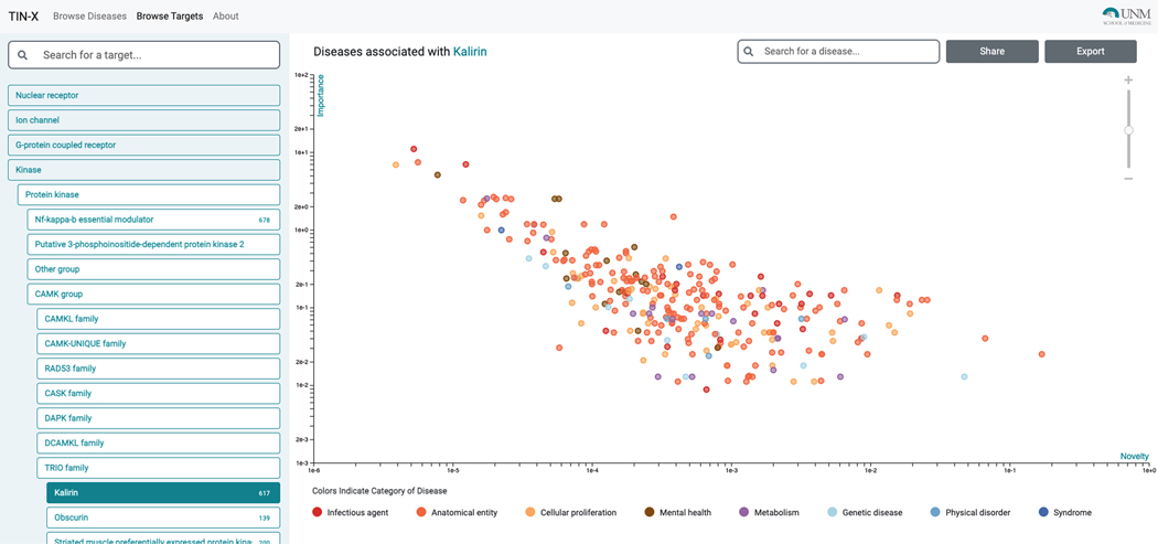
Searching by target name is supported. Diseases with stronger associations (higher Importance) are in the upper part of the plot, while diseases with a higher number of publications (lower Novelty) are on the left side of the plot. Diseases that are likely of most interest are plotted in the upper-right area of the plot (Figure 71).
10
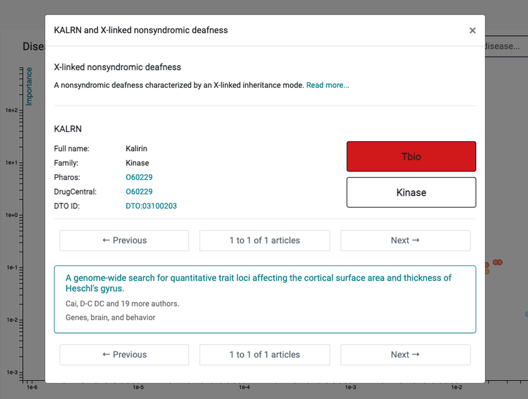
The plot, however, remains target-centric. Upon clicking on a point, the disease name and protein name are displayed, with appropriate links to Pharos and DrugCentral (Figure 72).
11
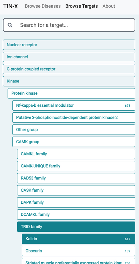
When selecting a target family (e.g., kinase), the user can drill down to the desired level of granularity, before examining disease associations for a specific protein. Starting from Kinase, for example, the user must click Protein kinase → CAMK group → TRIO family → Kalirin, before diseases associated with Kalirin (KALRN) are displayed (Figure 70).
12
The top disease (highest Importance, lowest Novelty) associated with KALRN is “disease by infectious agent”, followed by “psychotic disorder”. We recommend repeated scrolling before identifying a leaf term corresponding to the Disease Ontology. For example, next to “psychotic disorder” is “schizophrenia” (a child term); this association is supported by 26 publications, including Miller et al. (Miller et al., 2017). The most novel association (lowest Importance) is for “X-linked nonsyndromic deafness” (Figure 72), supported by Cai et al. (Cai et al., 2014). This association is genuine, as the gene name (KALRN) is mentioned in the abstract, in relation to the rs333332 SNP.

Figure 70. — Starting with the superfamily Kinase, the user can further refine the selection to Protein kinase → CAMK group → TRIO family → Kalirin by using the left navigation pane within Browse Targets.

Figure 71. — Within “Browse Targets”, diseases associated with Kalirin (KALRN) are plotted with log–log Importance–Novelty axes, and are colored according to the top hierarchical Disease Ontology term.

Figure 72. — For the example target Kalirin (KALRN), the most novel association (lowest Importance) is for “X-linked nonsyndromic deafness”. This detailed view includes the full name and family of the target, links to Pharos and DrugCentral, and in this case, the one article responsible for this association between KALRN and X-linked nonsyndromic deafness.

Sharing and downloading data

13
Whether in “Browse Diseases” or “Browse Targets” mode, the user can share data in two ways. First, for any given plot, the specific URL (universal resource locator) for that visualization can be copied and shared with third-party users. This can be done by clicking on the “Share” button. Second, the data can be exported (in comma-separated value format), and thus archived or post-processed with third-party software. Exported data includes Novelty and Importance scores, in addition to Disease names and identifiers in the “Browse Targets” mode, as well as Target names and identifiers in the “Browse Diseases” mode, respectively.

Basic Protocol 7: Interacting with the DrugCentral user interface

DrugCentral is an online compendium (Ursu et al., 2017) centered on “active pharmaceutical ingredients” and their link to “pharmaceutical products”. DrugCentral distills relevant information from “pharmaceutical product” (or formulation) package inserts; while these are frequently referred to as “drugs” by patients and medical practitioners, herein we reserve the term “drugs” for “active pharmaceutical ingredients”. All data, including downloads, related to DrugCentral can be accessed at its designated web portal (https://drugcentral.org/). DrugCentral provides information on active ingredients, chemical entities, pharmaceutical products, drug mode of action, medical uses (indications, contra-indications and off-label uses), pharmacologic action, as well as adverse events (Ursu et al., 2019). As of 2021, DrugCentral (Avram et al., 2021) separately stores adverse events for women and men, and provides regulatory information extracted from the FDA Orange Book. DrugCentral is current (as of the date of the release) with regulatory approvals from the United States (US FDA), the European Union (EMA), Japan (PDMA) and, more recently, some drugs approved in China and Russia. Limited information on drugs that have been discontinued or withdrawn is available, particularly for drugs approved outside the US when package inserts and relevant information are not in English.

Necessary Resources

Hardware

Desktop or a laptop computer, or a mobile device, with a 100 Mbps or higher (fast) Internet connection.

Software

An up-to-date web browser such as Google Chrome (https://www.google.com/chrome/), Mozilla Firefox (https://www.mozilla.org/en-US/firefox/), Apple Safari (https://www.apple.com/safari/), or Microsoft Edge (https://www.microsoft.com/en-us/edge).

Protocol steps and annotations

Queries Supported by DrugCentral

Navigate to the DrugCentral portal (https://drugcentral.org/).
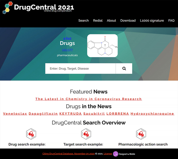
The main DrugCentral search bar supports three types of queries: drug, target and disease. Each of these will filter and prioritize results according to a 4-level ranking system ordered from highest to lowest, as follows:
- a
  query term matching drug name or synonyms mechanism of action target, or drug indication (see below).
- b
  query term matching disease term in drug contraindications or off-label uses, targets listed in drug bioactivity profiles (not MoA targets), or pharmacologic action descriptions.
- c
  query term matching the short drug description text.
- d
  query term matching full text in the FDA drug labels processed from DailyMed (Figure 73).
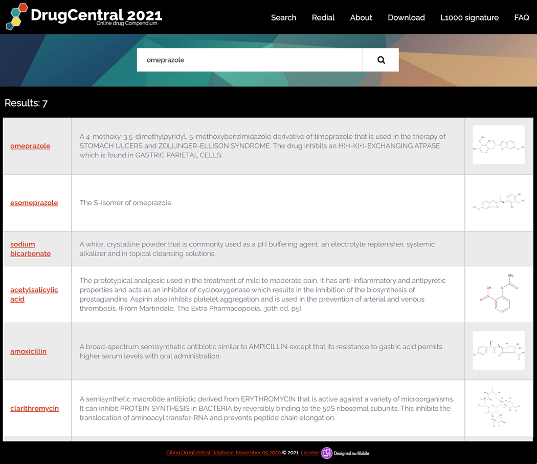
For example, drug query results are sorted to display active ingredients first (e.g., omeprazole), followed by related ingredients (e.g., esomeprazole) and by other active ingredients that are co-formulated with the queried substance into pharmaceutical products. A query by brand name (e.g., prilosec) includes other antacids such as sodium bicarbonate, antibiotics such as amoxicillin and clarithromycin (co-prescribed with omeprazole to treat stomach ulcers caused by Helicobacter pylori) as well as acetyl-salicylic acid, which is combined with omeprazole for the prevention of stroke. (Figure 74)
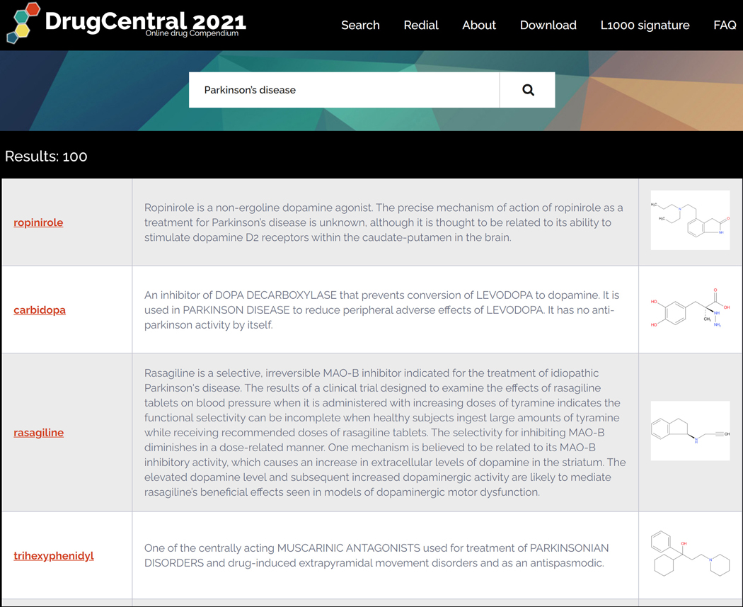
Disease names are mappable to multiple terminologies such as Disease Ontology, MeSH, SNOMED-CT and MedDRA. Disease term queries first retrieve indications, followed by off-label and contra-indications, then other sections (e.g., side effects) that contain medical / disease terms. For example, the query “Parkinson’s disease” (PD) first lists drugs indicated for PD (e.g., ropinirole), followed by drugs indicated in complications of PD (e.g., fludrocortisone is indicated for the PD-associated orthostatic hypotension), then by drugs that list PD as side-effect (e.g., dimenhydrinate) (Figure 75).
Target name queries support input as text (e.g., “muscarinic m1”), gene symbol (CHRM1) or UniProt (P11229) and SwissProt (ACM1_HUMAN) identifiers. It is recommended to use the exact target names adopted by UniProt, though gene/protein identifiers are preferred.

Figure 73. — DrugCentral homepage. DrugCentral search bar supports three types of queries: drug, target and disease.

Figure 74. — DrugCentral search results for “Omeprazole” first lists drugs indicated for “Omeprazole” (e.g., sodium bicarbonate) followed by drugs indicated in complications.

Figure 75. — Drugcentral query result for “Parkinson’s disease” (PD) first lists drugs indicated for PD (e.g., ropinirole), followed by drugs indicated in complications of PD (e.g., fludrocortisone is indicated for the PD-associated orthostatic hypotension), then by drugs that list PD as side-effect (e.g., dimenhydrinate).

Queries Supported by DrugCentral: Redial

5
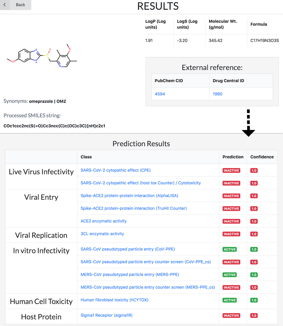
Given its basic science focus, the machine-learning based REDIAL-2020 platform (Kc et al., 2021), which is also part of DrugCentral, supports queries by drug name (e.g., omeprazole), by PubChem compound identifier (e.g., 4594) or by chemical structure in the SMILES (Weininger, 1988) format (e.g., COc1ccc2nc(S(=O)Cc3ncc(C)c(OC)c3C)[nH]c2c1). Regardless of format, all input queries for REDIAL-2020 are converted to SMILES format in order to predict anti-viral properties (Figure 76). See also Protocol nr 8.

Figure 76. — DrugCentral Redial query result for Omeprazole. All input queries for REDIAL-2020 are converted to SMILES format in order to predict anti-viral properties.

Queries Supported by DrugCentral: L1000

6
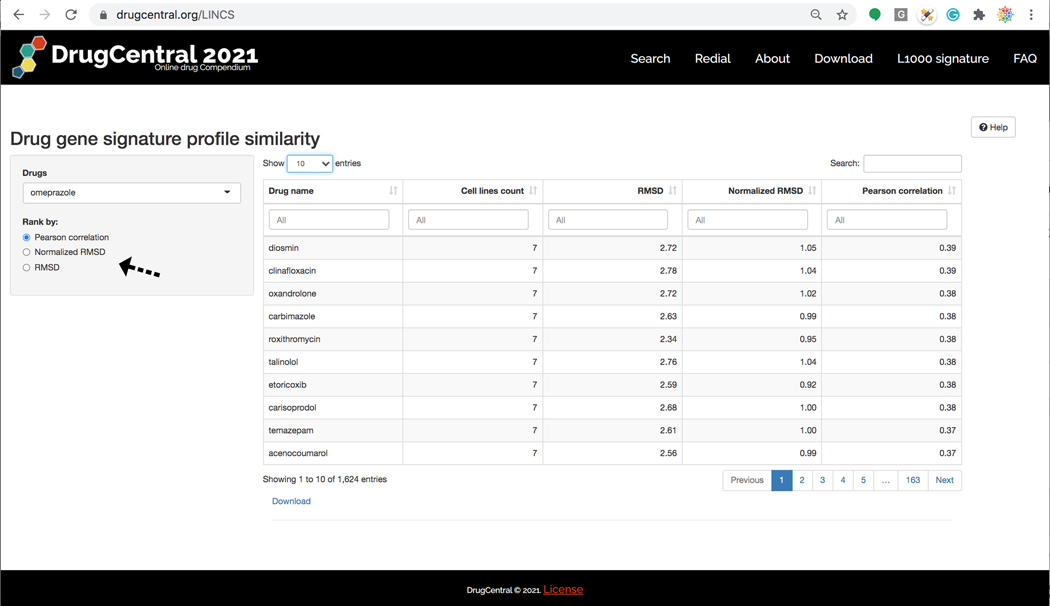
The other search interface available in DrugCentral, implemented in R-Shiny https://shiny.rstudio.com/) supports browsing and searching for drug names for which gene perturbation profiles were recorded across one more of the 81 cell lines collected during the LINCS (Library of Integrated Cellular Signatures) project. Based on the L1000 perturbation profiles for 1613 drugs, the L1000 DrugCentral app allows users to query (via drug names) which drugs have the most similar gene perturbation profiles, ranked by cell lines (Figure 77).

Figure 77. — The L1000 search input home page. The L1000 DrugCentral app allows users to query (via drug names) which drugs have the most similar gene perturbation profiles, ranked by cell lines.

DrugCentral Drugcards: A step-by-step content guide

7
At its core, DrugCentral is a drug-centric resource. Thus, all queries are likely to provide information that is displayed in the form of “drug cards”. Data elements identified when searching a drug by name would be thus retrieved in a similar manner when searching by target or by disease, as both queries result in lists of drug cards.
8
Each drug card can be directly accessed (linked out) by observing the following (specific) format:

https://drugcentral.org/drugcard/<DrugcentralStruct.ID>

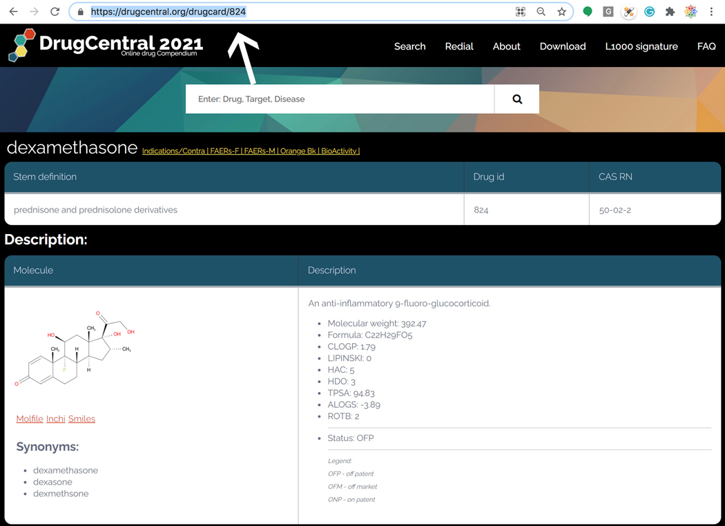
where “DrugcentralStruct.ID” is the DrugCentral structure ID number. For example, DrugcentralStruct.ID=824 resolves to dexamethasone. This manner of mining drug cards is not intended for casual users. Rather, this format is intended for programmatic access to DrugCentral content (Figure 78).
9
What follows is a “section by section” guide to drug card content, shown by section title. These are not intended as comprehensive explanations, but rather as brief illustrations of the diverse content available through DrugCentral.
10
“Stem definition” displays International Nonproprietary Names (INN), which are associated with “pharmacologically related groups”; that section also displays Chemical Abstract Services (CAS) registry numbers, in addition to DrugCentral IDs.
11
“Description” depicts the two-dimensional chemical structure (as well as three separate chemical structure file formats), a number of synonyms and computed chemical descriptors such as Lipinski’s “rule of 5”. (Lipinski et al., 2001) The intellectual property / regulatory status of the drug (if available) is also shown under “Status”, with one of 3 options: OFP - off patent; OFM - off market; and ONP - on patent, respectively (Avram et al., 2020).
12
“Drug dosage” provides a sample (typically, the “maximum dose strength”) of the dosages available for oral / non-oral formulations of the drug.
13
“ADMET Properties” - Absorption, Distribution, Metabolism, Excretion and Toxicity - provides experimental ADMET values, when available. These properties are half-life, systemic clearance, volume of distribution at steady state and fraction unbound, all intravenous pharmacokinetic parameters (Lombardo et al., 2018); the fraction excreted unchanged in urine (extent of metabolism), water solubility and their composite parameter BDDCS, Biopharmaceutical Drug Disposition Classification System, as discussed elsewhere (Benet et al., 2011); and MRTD, the Maximum Recommended Therapeutic Daily Dose (Contrera et al., 2004).
14
“Approvals” shows the date of approval by regulatory agencies (if available).
15
“FDA adverse event reporting system (Female)”, followed by “FDA Adverse Event Reporting System (Male)” lists adverse events, separated by sex, in the decreasing order of the likelihood ratio (Huang et al., 2011).
16
“Pharmacologic action” highlights the drug annotations corresponding to (sometimes multiple) ATC (Anatomical, Therapeutic and Chemical) classification system codes - ATC codes are available at (WHOCC); chemical ontology information from ChEBI(EBI Web Team); FDA terminology; and MeSH (Medical Subject Headings) terms(MeSH Browser).
17
“Drug use” lists indications, off-label use and contra-indications, mapped to SNOMED-CT (Bhattacharyya, 2016) and DOID (Disease ontology - institute for genome sciences @ university of Maryland), where available. Drug indications and contra-indications are mined from package inserts (drug labels), whereas off-label uses are from literature.
18
“Acid dissociation constants calculated using MoKa v3.0.0” shows calculated acid/base dissociation constants, as calculated with the MoKa software (Milletti et al., 2010).
19
“Orange Book patent data (new drug applications)” and “Orange Book exclusivity data (new drug applications)” complement DrugCentral information on marketed pharmaceutical formulations by adding FDA Orange Book(Orange book: Approved drug products with therapeutic equivalence evaluations) for patents, as well as exclusivity data, for new drug applications.
20
“Bioactivity Summary” distils information from multiple bioactivity databases, e.g., ChEMBL (Mendez et al., 2019) and the IUPHAR Guide to Pharmacology (Armstrong et al., 2019), in addition to scientific literature and information from drug labels. Numeric information is converted to the negative log molar of the effective drug concentration at measurement. Mechanism-of-action drug targets (Santos et al., 2017) are marked separately.
21
The “External reference” section contains drug identifiers used by other on-line resources. This section includes identifiers used in medical practice, such as the Veterans Health Administration (e.g., VHA unique identifier, VUID), the National Drug File reference terminology (NDFRT, (National drug file - reference terminology source information, 2016) and RxNorm (RxNorm, 2004), as well as identifiers used by PubChem, ChEBI, DrugBank, etc.
22
Last but not least, the “Pharmaceutical products” section provides direct links to DailyMed (DailyMed, 2015), while incorporating simple meta-data descriptors such as “category” (e.g., prescription vs. over-the-counter), number of ingredients, administration route, etc. This section also includes a clickable container that captures the full text (no images) of the FDA approved package insert.

DrugCentral Accession “DrugcentralStruct.ID” for cross referencing DrugCentral drug cards.

DrugCentral Target Cards: A step-by-step content guide

23
In Addition to DrugCentral’s Drugcards, a set of Target Cards can be directly accessed by observing the following (URL) syntax: https://drugcentral.org/target/<UniprotAccession.ID>
24
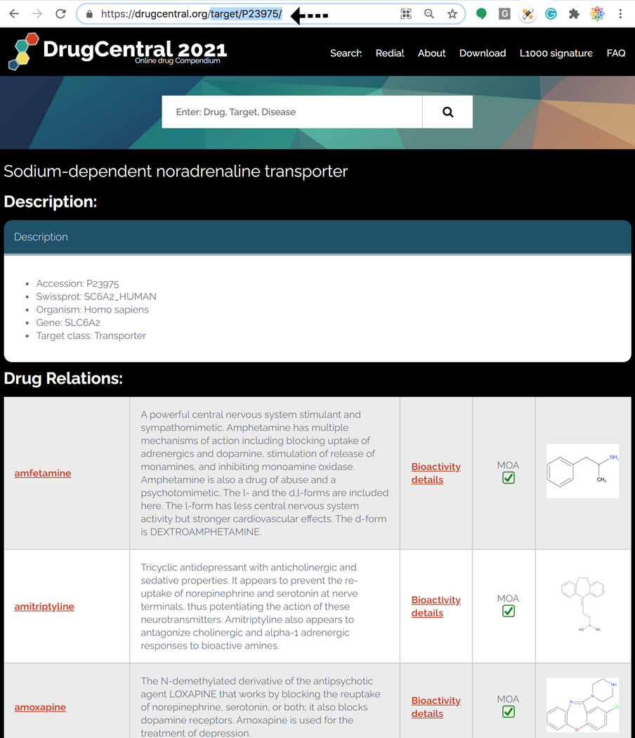
For example, https://drugcentral.org/target/P23975/ resolves to Sodium-dependent noradrenaline transporter. This method of mining Target Cards is not intended for casual users. Rather, this format is intended for programmatic access to machine readable Target metadata (Figure 79).
25
What follows is a “section by section” guide to Target card content and target metadata.
26
“Description” depicts the Accession ,Swissprot, Organism, Gene & Target class followed by Drug relations where the Drugs Bioactivity mechanism-of-actions are identified and marked.
27
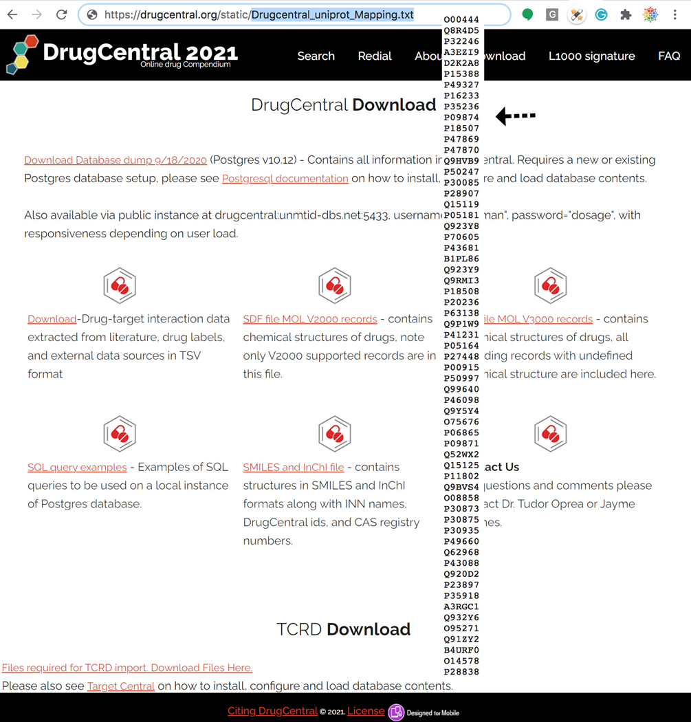
To retrieve all cross-referenced Drug Central Targetcards cards mapped to Uniprot Accession Ids use the following (machine readable) URL syntax (Figure 80): https://drugcentral.org/static/Drugcentral_uniprot_Mapping.txt

Figure 79. — DrugCentral’s Target Card. Target card depicts Accession, Swissprot, Organism, Gene & Target class followed by Drug relations where the Drugs Bioactivity mechanism-of-actions are marked.

Figure 80. — Uniprot Accession IDs used for crossrefrencing and machine querying DrugCentral Targetcards. **https://drugcentral.org/static/Drugcentral_uniprot_Mapping.txt**

Additional information

28
The “Download Database dump 9/18/2020 (Postgres v10.12)” option contains all the information stored in DrugCentral. It requires a new or existing Postgres database setup. Users are directed to consult the Postgresql documentation on how to install, configure and load database contents. This is also available via public instance at drugcentral:unmtid-dbs.net: 5433, username=“drugman”, password=“dosage”, with responsiveness depending on user load.

Example queries to extract subsets of data from DrugCentral. Requires a local instance of DrugCentral loaded into a PostgreSQL database. To load the DrugCentral database dump assuming PostgreSQL is up and running and the user has admin privileges, run in PostgreSQL.

#create database drugcentral and then run using the OS shell
$gunzip -c drugcentral.dump.06212018.sql.gz | psql drugcentral
#Example 1: Select Off-patent drugs that bind to “Mast/stem cell growth factor #receptor Kit” as mode-of-action target” in DrugCentral’s Postgres Db.
-select
 distinct(structures.name) as drug_name
  from
 structures
  join act_table_full on structures.id = act_table_full.struct_id
  Where
   structures.status =‘OFP’ and
 act_table_full.moa = 1 and
 act_table_full.target_name = ‘Mast/stem cell growth factor receptor Kit’
#Example 2: Select drugs indicated for seasonal allergic rhinitis that have #the lowest LLR for somnolence in males.
 -select
 distinct(structures.name) as drug_name,
   faers_male.*
   from
   structures
   join struct2atc on structures.id = struct2atc.struct_id
   join atc on struct2atc.atc_code = atc.code
   join faers_male on structures.id=faers_male.struct_id
 Where
  atc.l2_name = ‘ANTIHISTAMINES FOR SYSTEMIC USE’ and
  faers_male.meddra_name = ‘Somnolence’ and
  faers_male.llr <= 2*faers_male.llr_threshold
  order by
  faers_male.llr asc

30
To download additional example SQL queries for extracting subsets of data from DrugCentral use the following URL: https://unmtid-shinyapps.net/download/example_query.sql

Basic Protocol 8: Estimating Anti-SARS-CoV-2 activities with DrugCentral REDIAL-2020

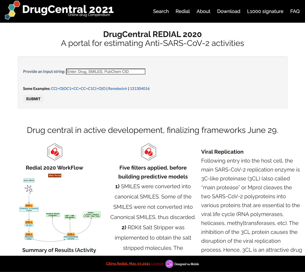
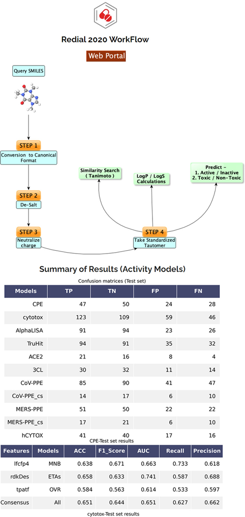
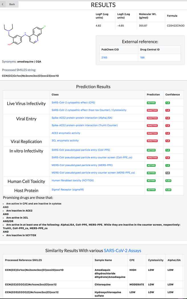
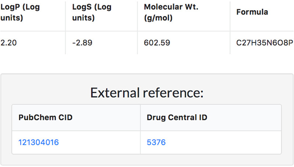
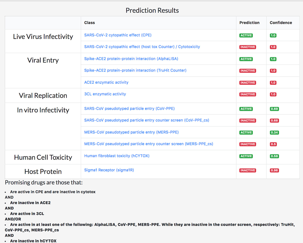
There is currently an urgent need to find effective drugs for treating coronavirus disease 2019 (COVID-19). DrugCentral REDIAL-2020 (Kc et al., 2020), is a suite of machine learning models that forecast activities for live viral infectivity, viral entry, and viral replication specifically for severe acute respiratory syndrome coronavirus 2 (SARS-CoV-2), in vitro infectivity, and human cell toxicity. This application serves the scientific community when prioritizing compounds for in vitro screening and may ultimately accelerate identifying novel drug candidates for COVID-19 treatment. REDIAL-2020 consists of eleven independently trained machine learning models using high throughput screening data from the NCATS COVID19 portal (https://opendata.ncats.nih.gov/covid19/index.html) and includes a similarity search module that queries the underlying experimental dataset for similar compounds. These models were developed using experimental data generated by the following assays: the SARS-CoV-2 cytopathic effect (CPE) assay and its host cell cytotoxicity counterscreen, the Spike–ACE2 protein–protein interaction (AlphaLISA) assay and its TruHit counterscreen, the angiotensin-converting enzyme 2 (ACE2) enzymatic activity assay, the 3C-like (3CL) proteinase enzymatic activity assay, the SARS-CoV pseudotyped particle entry (CoV-PPE) assay and its counterscreen (CoV-PPE_cs), the Middle-East respiratory syndrome coronavirus (MERS-CoV) pseudotyped particle entry assay (MERS-PPE) and its counterscreen (MERS-PPE_cs), and the human fibroblast toxicity (hCYTOX) assay (Figure 81).

Figure 81. — Redial Home page with Search SMILES, drug names and PubChem CIDs enabled.

Necessary Resources

Hardware

Desktop or a laptop computer, or a mobile device, with a 100 Mbps or higher (fast) Internet connection.

Software

An up-to-date web browser such as Google Chrome (https://www.google.com/chrome/), Mozilla Firefox (https://www.mozilla.org/en-US/firefox/), Apple Safari (https://www.apple.com/safari/), or Microsoft Edge (https://www.microsoft.com/en-us/edge)

Protocol steps and annotations

Redial: A step-by-step content guide

1
By accessing REDIAL-2020 (http://drugcentral.org/Redial) from any web browser, including mobile devices, the submission page is displayed.
2
The web server accepts SMILES, drug names or PubChem CIDs as input. Regardless of input, the protocol converts drug names (from DrugCentral) or PubChem CIDs into SMILES.
3
The user interface provides a summary of the models, such as model type, which descriptor categories were used for training and the evaluation scores. The user interface depicts the processes of cleaning the chemical structures (encoded as SMILES) before training the machine learning models (Figure 82).
4
As an example, amodiaquine has been shown to have promising anti-SARS-CoV-2 behaviour in several papers (Bocci et al., 2020; Si et al., 2021), but its mechanism of action has not been well established yet. When given as an input to Redial, the webapp opens a new window with the predicted activities.
5
The prediction results table shows that amodiaquine is predicted to be active in cytopathic effect experiments while there are no clues on its mechanism (inactive in AlphaLISA, ACE2, 3CL assays) (Figure 83).
6
REDIAL-2020 links directly to DrugCentral for approved drugs and to PubChem for chemicals (where available), enabling easy access to further information on the query molecule (Figure 84).
7
Using REDIAL-2020 estimates, promising anti-SARS-CoV-2 compounds would ideally be active in the CPE assay while inactive in cytotox and in hCYTOX.

Figure 82. — Redial interface provides a summary of the models, such as model type, which descriptor categories were used for training and the evaluation scores. The user interface further depicts the processes of cleaning the chemical structures (encoded as SMILES) before training the machine learning models.

Figure 83. — Redial prediction results table with example search term “amodiaquine”. Amodiaquine is predicted to be active in cytopathic effect experiments while there are no clues on its mechanism (inactive in AlphaLISA, ACE2, and 3CL assays).

Figure 84. — REDIAL links directly to DrugCentral for approved drugs and to PubChem for chemicals (where available), enabling easy access to further information on the query molecule.

Queries Supported by Redial

8
Input queries such as drug name and PubChem CID are converted to SMILES before processing. Each SMILES string input is subject to four different steps, namely, converting the SMILES into canonical SMILES, removing salts (if present), neutralizing formal charges (except permanent ones) and standardizing tautomers. REDIAL-2020 predicts input compound activity across all eleven assays: CPE, cytotox, AlphaLISA, TruHit, ACE2, 3CL, CoV-PPE, CoV-PPE_cs, MERS-PPE, MERS-PPE_cs and hCYTOX (Figure 85).

Figure 85. — REDIAL-2020 results page predicting compound activity across all eleven assays: CPE, cytotox, AlphaLISA, TruHit, ACE2, 3CL, CoV-PPE, CoV-PPE_cs, MERS-PPE, MERS-PPE_cs, and hCYTOX.

Additional information

All of the codes and the trained models are available from: https://doi.org/10.5281/zenodo.4606720
The source code and specific models are available through Github at: (https://github.com/sirimullalab/redial-2020), or via Docker Hub (https://hub.docker.com/r/sirimullalab/redial-2020) for users preferring a containerized version. All the pre-ML processing and “data cleaning” scripts are here: https://github.com/sirimullalab/redial-2020/tree/master/data-cleaning
All workflows and procedures were performed using the KNIME platform 10. The NCATS data associated with the aforementioned assays were downloaded from the COVID-19 portal. https://opendata.ncats.nih.gov/covid19/assays

Basic Protocol 9: Drug Set Enrichment Analysis using Drugmonizome

Drugmonizome (Kropiwnicki et al., 2021) serves processed data extracted from drug and small molecule databases available from a variety of online repositories and data portals. The processed data is provided in the form of drug set libraries which serve as the underlying database for drug set enrichment analysis. Drugmonizome enables users to submit lists of drugs and small molecules as the input query. These drug sets are compared against various drug set libraries that contain known associations between drugs and their attributes, for example, side effects, indications, targets, pathways, induced gene expression signatures, and other attributes. Additionally, Drugmonizome provides options for querying metadata associated with drug sets to find relevant drugs, small molecules, and drug sets for a given free text query.

Necessary Resources

Hardware

Desktop or a laptop computer, or a mobile device, with a fast Internet connection

Software

An up-to-date web browser such as Google Chrome (https://www.google.com/chrome/), Mozilla Firefox (https://www.mozilla.org/en-US/firefox/), Apple Safari (https://www.apple.com/safari/), or Microsoft Edge (https://www.microsoft.com/en-us/edge).

Protocol steps and annotations

Metadata Search

Navigate to the Drugmonizome homepage (https://maayanlab.cloud/drugmonizome/). The metadata search is displayed by default. Using the search bar, query terms of interest to identify resources, drug set libraries, drug sets, and small molecules contained in Drugmonizome. Example terms are suggested for each type of metadata search (Figure 86).
Alternate between resource, drug set library, drug set, and small molecule metadata searches by clicking the corresponding tab. When performing metadata searches for drug sets, use the filter table to query terms within specific resources, drug set libraries, and association types.
Upon submitting a term of interest using the search bar, a list of results that match the term is displayed (Figure 87).
Clicking on any term displays a page with identifying metadata for the resource, drug set library, drug set, or small molecule. When perusing drug set metadata, a search bar exists for querying specific small molecules of interest within the set (Figure 88).

Figure 86. — Drugmonizome metadata search page with drug set search enabled.

Figure 87. — Drugmonizome metadata search page with example term “Headache” queried using the search bar.

Figure 88. — Drug set page that includes identifying metadata for the drug set and the small molecules included in the drug set. The search bar can be used to query specific drugs or small molecules of interest.

Drug Set Enrichment

1
Navigate to the drug set enrichment page by clicking the corresponding tab on the website header. The drug set enrichment page includes a search box where a list of drugs and small molecules can be pasted. The page also includes several example drug sets that are pasted into the box when clicked (Figure 89). As an example, click the “69 in vitro COVID-19 hits from a drug screen by Ellinger et al.” link to populate the search box with a small molecule set.

Note: Drug and small molecule entities can be queried by name, DrugBank IDs, Broad Institute Accession Numbers (BRD-IDs), SMILES strings, and InChIKeys.
2
Click the “Perform Drug Set Enrichment Analysis” button and a results page of all resources with enriched terms is returned. Each of the resources with enriched drug set libraries are represented as an icon with the number of enriched terms for each resource (Figure 90).
3
Click on any of the resource icons to be redirected to a page with the top enrichment results for each drug set library represented by a toggleable bar graph or scatter plot. The drug set library enrichment results can be expanded by clicking the corresponding button (Figure 91).
4
The expanded page includes the scatter plot, bar graph, and table view of the top enriched terms. The table representation displays the top enriched terms and their p-values, odds ratio, and corrected q-values. Terms of interest can be queried using the search bar above the table. The table is also available for download as a .TSV file (Figure 92).

Figure 89. — Drug set enrichment page with the “Ellinger et al.” example drug set pasted into the search box.

Figure 90. — Enrichment results page after submitting the “Ellinger et al.” example drug set. Each resource is represented by an icon and the number of enriched drug sets from each resource are displayed above the icon.

Figure 91. — After clicking on the SIDER resource, the top enriched terms from both drug set libraries from SIDER are displayed side by side. Bar charts and scatter plots visualize the top enriched terms. The view for a particular library can be expanded by clicking the “expand” button.

Figure 92. — Expanded view for the SIDER Side Effects drug set library. This view includes the bar chart of top enriched terms, scatter plot of top enriched terms, and table of top enriched terms with each of their p-values, odds ratios, overlap sizes, and corrected q-values.

Resources Pages

5
Navigate to the resources page by clicking the corresponding tab on the website navigation bar (Figure 93).
6
Each of the drug data resources used to create drug set libraries is catalogued on this page. Click on the DrugBank resource card to view metadata specific to DrugBank, as well as drug set libraries curated from DrugBank (Figure 94).
7
Click on the “DrugBank Small Molecule Targets” library to be redirected to a page with identifying metadata for the drug set library. The metadata for the drug set library includes download links for the .DMT files in drug name or InChIKey format (Figure 95). Additionally, each of the drug sets included in this library are listed below. Clicking on any drug set name redirects to a page with metadata specific to the drug set, as well as the set of associated small molecules.

Figure 93. — The resource page listing all drug data resources included in Drugmonizome.

Figure 94. — Expanded view of the DrugBank resource with identifying metadata and drug set libraries curated from DrugBank.

Figure 95. — Expanded view of the DrugBank Small Molecule Targets drug set library with metadata that include download links for the DMT file in drug name and InChIKey formats. All drug sets included in the library are listed below and each drug set can be expanded to view drug set specific metadata and the list of small molecules included in the drug set.

Basic Protocol 10: The Drugmonizome-ML Appyter

A wealth of data from a multitude of sources is readily available for thousands of bioactive small molecules in Drugmonizome (Kropiwnicki et al., 2021). The information in Drugmonizome can be harnessed to develop machine learning models that utilize such data to predict the properties of small molecules that are poorly annotated. The Drugmonizome database draws upon a variety of publicly available resources to label each small molecule by its associations with pathways, protein targets, induced gene expression profiles, chemical features, and other attributes. Drugmonizome-ML is an Appyter (Clarke et al., 2021) that executes a machine learning pipeline as a Jupyter notebook using the data curated for creating Drugmonizome. Drugmonizome-ML can be used to make predictions for indications and other attributes such as drug targets or side effects for poorly annotated pre-clinical bioactive small molecules.

Necessary Resources

Hardware

Desktop or a laptop computer, or a mobile device, with a fast Internet connection

Software

An up-to-date web browser such as Google Chrome (https://www.google.com/chrome/), Mozilla Firefox (https://www.mozilla.org/en-US/firefox/), Apple Safari (https://www.apple.com/safari/), or Microsoft Edge (https://www.microsoft.com/en-us/edge).

Protocol steps and annotations

Input Dataset Selection

1
Navigate to the Drugmonizome-ML Appyter (https://appyters.maayanlab.cloud/Drugmonizome_ML/). The input form is divided into three sections: input dataset selection, target label selection, and machine learning pipeline.
2
Select datasets from Drugmonizome and SEP-L1000 (Kropiwnicki et al., 2021; Wang et al., 2016) to populate the feature matrix that will be used for learning and classification. Each of the datasets’ contents are described using tooltips (Figure 96). For the demonstration, select the “LINCS Gene Expression Signatures” from the “Transcriptomic and Imaging Datasets” subfield and “Morgan Fingerprints” from the “Chemical Fingerprints Generated for Compounds from SEP-L1000” subfield.
3
Additional options for pre-processing the feature matrix are available. If selecting features from various data sources, it is likely that not all compounds will be included across all feature sets, therefore a toggleable option decides whether drugs with missing data are retained or dropped from the feature matrix. Additionally, because some of the available feature sets are binary association matrices, there is the option to apply TF-IDF normalization to account for frequency of common and rare features among the small molecules (Figure 97). In general, the default settings for these options are recommended.

Figure 96. — Input dataset selection section of the Drugmonizome-ML Appyter. Each input dataset is annotated with tooltips.

Figure 97. — Toggleable options for deciding whether to retain or drop drugs with missing data and TF-IDF normalization.

Target Label Selection

4
In this section, select the positive class label for a binary classification problem. There is the option to select an attribute from any of the Drugmonizome drug set libraries in an autocomplete field where relevant drug-set labels from Drugmonizome are offered as potential class labels (Figure 98). Type any characters into the autocomplete field and matching drug-set labels will be displayed. For the demonstration, type “neuropathy peripheral (from SIDER Side Effects)” into the autocomplete field.
5
Alternatively, upload a newline separated .txt file of compounds to be used as positive examples of a class to predict by selecting the “List” option in the “Target Label Selection” section. Example .txt files are available for download to understand the structure of the file (Figure 99). Choose the drug identifier format (drug name or InChI key) that small molecules within the text file are described by. InChI Keys are the recommended format.
6
The “Include stereoisomers” option decides whether to match compounds from the feature matrix to the target vector using the first 14 characters of the InChIKey (which encodes chemical connectivity) thus including stereoisomers of a particular small molecule, or whether to consider only one form of a molecule and match by the whole InChIKey.

Figure 98. — Target label selection with “Attribute” selected. The autocomplete field can be populated with search terms that match to drug-set labels in Drugmonizome which will be used as the positive class to predict.

Figure 99. — Target label selection with “List” selected. Newline separated .txt files can be uploaded with small molecules that are part of a positive class to predict. The drug identifier format drop-down menu allows specification of how small molecules are catalogued within the uploaded file (names or InChI key).

Machine Learning Pipeline

7
In this section, select data visualization options, machine learning classifiers, machine learning hyperparameters, and methods to evaluate the classifier (Figure 100).
8
Select your preferred data visualization method from the drop-down menu under the “Data Visualization Method” field. The default and recommended method is UMAP.
9
If applicable, select a dimensionality reduction algorithm from the drop-down menu under the “Dimensionality Reduction Algorithm” field.
10
If applicable, select a feature selection method from the drop-down menu under the “Machine Learning Feature Selection” field.
11
The “Machine Learning Algorithm” section includes 9 distinct classifiers that can be chosen by clicking on the corresponding classifier name. Furthermore, each classifier has hyperparameter fields that can be modified. For example, select the “Extra Trees classifier”. Input “1250” in the “n_estimators” field. Select “entropy” in the “criterion” drop-down menu. Select “log2” in the “max_features” drop-down menu. All other hyperparameters can be kept as default.
12
Select whether to calibrate algorithm predictions by selecting the appropriate choice in the “Calibrate algorithm predictions” field. This setting will calibrate the predictions output by the chosen model, eliminating model-imparted bias. It is recommended to keep this setting as default.
13
Select a cross-validation method from the drop-down menu under the “Cross-Validation Algorithm” field. The recommended option is Repeated Stratified Group K-Fold because this cross-validation method will maintain class ratios across train and validation splits. Furthermore, choose the number of cross-validation folds and cross-validation repetitions in the subsequent fields. For the demonstration, input “10” into the “Number of Cross-Validation Folds” field and “3” into the “Number of Cross-Validated Repetitions” field.
14
Choose the primary evaluation metric for assessing the performance of the model from the drop-down menu under the “Primary Evaluation Metric” field. The default and recommended metric is “roc_auc”.
15
Choose any additional evaluation metrics from the drop-down menu under the “Evaluation Metrics” field and these metrics will also be reported for the trained model.
16
Click “Submit” at the bottom of the input form.

Figure 100. — Machine learning pipeline section with methods for data visualization, machine learning classifier selection, hyperparameter settings, and metrics to evaluate the classifier.

Navigating the Drugmonizome-ML Appyter Notebook

17
A Jupyter Notebook will begin executing in the cloud once the input form is submitted. The notebook includes an option to download the notebook, toggle displaying the code, and run the notebook locally. Additionally, a table of contents exists with clickable elements that link to specific sections within the notebook (Figure 101).
18
Scroll down to the “Select Input Datasets and Target Classes” section or click on the corresponding section from the table of contents. The feature matrix that was generated based on the selected features from the input form is displayed. The feature matrix is composed of 19,898 compounds and 3026 features from LINCS Gene Expression Profiles and TF-IDF normalized Morgan Fingerprints (Figure 102).
19
Additionally, information is displayed about how the target array is constructed, how many compounds from the target array are included in the feature matrix, and how many compounds were discarded because they were not included in the feature matrix. Unmatched compounds are available for download.
20
Navigate to the “Dimensionality Reduction and Visualization” section to view the input feature space using the dimensionality reduction and visualization methods that were selected in the input form. Positive class labels are labeled within the visualization to demonstrate how the class of interest is clustered in the feature space (Figure 103).
21
Navigate to the “Machine Learning” section to view the trained classifier and evaluations of the classifier’s performance. The receiver operating characteristic curve (Figure 104), precision-recall curve (Figure 105), and confusion matrix (Figure 106) are displayed. Click the hyperlinks in the figure headers to download the figures.
22
Navigate to the “Examine Predictions” section to view the predictions made by the model in addition to the distributions of mean probability estimates and t-statistics. Figures displaying the distribution of mean cross-validation predictions (Figure 107), distribution of t-statistics (Figure 108), a UMAP visualization of the feature space with overlaid predictions (Figure 109), and a filterable table of the top predicted compounds (Figure 110) are displayed. Click the hyperlinks in the figure and table headers to download the corresponding figure or table.
23
Navigate to the “Feature Importance” section to view the most important features from the input feature matrix that were used to make predictions. A table of the most important features used by the model to make predictions (Figure 111), as well as a figure depicting the distributions of average and cumulative sum of feature importance (Figure 112) are displayed. Click the hyperlinks in the figure and table headers to download the corresponding figure or table.

Figure 101. — (1) To learn more about Appyters, click any of the header tabs to navigate to information pages. (2) Clickable options to download the Jupyter Notebook, toggle code when viewing the notebook, as well as the option to run the notebook locally. (3) Table of contents with clickable elements that link to a specific section within the notebook.

Figure 102. — Input dataset visualized in Dataframe format. The number of matched compounds in the target vector is displayed, along with a downloadable .txt file of unmatched compounds.

Figure 103. — Dimensionality Reduction and Visualization Section with input feature space visualized using UMAP.

Figure 104. — Receiver Operating Characteristic (ROC) curves of classifier performance after cross-validation splits.

Figure 105. — Precision-recall (PR) curves of classifier performance after cross-validation splits.

Figure 106. — Confusion matrix for cross-validation predictions from the trained classifier.

Figure 107. — Mean probability distribution for classifier predictions including compounds with known positive labels, unknown class labels, and a simulated null distribution.

Figure 108. — T-statistic distribution for classifier predictions including compounds with known positive labels, unknown class labels, and a simulated null distribution.

Figure 109. — UMAP dimensionality reduction of the input feature space with predicted compounds overlayed. The color of each point corresponds to the mean predicted probability, whereas the size of the point corresponds to the significance of the probability.

Figure 110. — Table of the top predicted compounds ranked by prediction probability.

Figure 112. — Feature importance graphs with distribution scores for each feature and a cumulative distribution score across all features.

Basic Protocol 11: The Harmonizome-ML Appyter

Harmonizome (Rouillard et al., 2016) is a collection of processed datasets that abstract knowledge about genes and proteins. Using the processed data from Harmonizome, Harmonizome-ML enables interactive imputation of knowledge about the function and other properties of genes and proteins using machine learning. Combined with a user-friendly interface of an Appyter (Clarke et al., 2021) – a web-based software application enabling users to execute bioinformatics workflows without coding – the Harmonizome-ML Appyter can be used to build and evaluate machine learning pipelines with Harmonizome data in an accessible way. The Harmonizome-ML Appyter asks users to select or upload attributes for learning as well as specify a target vector to predict. Users also need to select from various machine learning algorithms and performance evaluation methods. Once these options are selected, the workflow is executed, and the results are presented as a Jupyter Notebook that is shareable and downloadable.

Necessary Resources

Hardware

Desktop or a laptop computer, or a mobile device, with a fast Internet connection

Software

An up-to-date web browser such as Google Chrome (https://www.google.com/chrome/), Mozilla Firefox (https://www.mozilla.org/en-US/firefox/), Apple Safari (https://www.apple.com/safari/), or Microsoft Edge (https://www.microsoft.com/en-us/edge).

Protocol steps and annotations

Navigating the input page

1
Navigate to the Harmonizome-ML Appyter (https://appyters.maayanlab.cloud/#/harmonizome_ml). The input form is divided into two sections: “attribute and prediction class dataset selection” and “settings”.
2
In the “Attribute and Prediction Class Selection” section, select attributes by clicking on the check box to the left of an attribute of choice; a blue check mark indicates that an attribute has been selected. Users may opt to upload a custom attribute dataset using the “Browse” button as well. Target selection can be from Harmonizome or customized; click on the text for the target selection desired and customize the class in the text box below (Figure 113).
3
The “Settings” section includes settings for various algorithms (dimensionality reduction, manifold projection, ML feature selection, cross validation, ML algorithm, hyperparameter search type, evaluation metrics) that can be customized. Simply click on the drop-down menu below an algorithm to view and update the options. For example, clicking on the drop-down menu for “Dimensionality Reduction Algorithm” displays the following options: PCA, truncated SVD, incremental PCA, ICA, and Sparse PCA. Click on the desired algorithm to use it for dimensionality reduction (Figure 114).
4
Once all selections have been made, click on the “Submit” button at the bottom of the page to run the analyses and generate the notebook.

Figure 113. — Attribute and Prediction Class Dataset Selection” section of the input form. Two datasets are selected to be used as features in the classifier algorithm. Hovering over tool tips displays information about each dataset. There is also an option to upload custom attribute datasets. The Target Selection subsection allows for selection of a class for the classifier to predict.

Figure 114. — Settings section including a variety of scikit-learn options for building the classifier as well as options for visualizing and evaluating classifier performance and predictions.

Navigating the notebook

5
Each notebook generated by the Harmonizome-ML Appyter includes explanations followed by code, data, and figures (both static and interactive). To download the notebook, toggle notebook code, or run the notebook locally, select the appropriate button at the top of the page. The notebook is divided into three sections (which can be accessed through the table of contents on the left side of the page): Inputs, Dimensionality Reduction, and Machine Learning (Figure 115).
6
Navigate to the “Inputs” section to view the feature matrix Dataframe generated from the datasets selected in the input form (Figure 116). Note that some Dataframes contain additional columns that can be explored by scrolling left to right. The first two Dataframes are individual datasets, whereas the final Dataframe displays the concatenated feature matrix that will be used for classification.
7
Scroll down to view the target array created from the dataset containing the class label to be predicted. Genes that are known to be associated with the class label are annotated with a 1, whereas genes not known to be associated with the class label are annotated with a 0 (Figure 117).
8
Navigate to the “Dimensionality Reduction” section. The process of dimensionality reduction involves transforming data from high-dimensional spaces to low-dimensional spaces without losing too much information. The input features are reduced using PCA and visualized in a 3D scatter plot (Figure 118). The reduced features are also projected onto a manifold with T-SNE (Figure 119).
9
Navigate to the “Machine Learning” section which features the machine learning pipeline assembled from the input form submission. A model is generated and trained via the customized pipeline and then used to predict genes that are strongly correlated with the target attribute. General explanations for the model’s performance are provided with ROC curves and a prediction matrix (Figure 120).
10
The prediction results are provided at the end of the pipeline and can be downloaded as a tab-separated (.tsv) file by clicking on “results.tsv” at the end of the notebook (Figure 121).

Figure 115. — Options to download the appyter notebook, toggle the code, and run the notebook locally. A table of contents on the left allows for navigating the various sections of the notebook.

Figure 116. — The input feature datasets visualized as Dataframes. The first and second Dataframes describe the “CCLE Cell Lines Gene Expression Profiles” and “ENCODE Transcription Factors Targets” datasets, respectively. The final Dataframe represents the concatenated feature matrix composed of the previous two datasets.

Figure 117. — Target array created from the “DISEASES Text-mining Gene-Disease Association Evidence Scores” dataset which contains the class label “cancer DOID:162”. Genes in the target array associated with the class label are marked with a 1, whereas genes that are not known to be associated with the class label are marked with a 0.

Figure 118. — 3D scatter plot of PCA reduced input features with genes associated with the target label are colored yellow.

Figure 119. — T-SNE visualization of the PCA reduced features.

Figure 120. — Receiver operating characteristic (ROC) curves and prediction matrix displaying model performance across cross-validation splits.

Figure 121. — Table of top genes predicted to be associated with the class label. The results table is available for download by clicking the “results.tsv” link.

Basic Protocol 12: GWAS target illumination with TIGA

Target Illumination GWAS Analytics (TIGA) (Yang et al., 2021) is a web application that facilitates drug target illumination by scoring and ranking protein-coding genes associated with traits from genome-wide association studies (GWAS). Similarly, TIGA can score and rank traits with the same gene-trait association metrics. Rather than a comprehensive analysis of GWAS for all biological implications and insights, this focused application provides a rational method by which GWAS findings can be aggregated and filtered for applicable, actionable intelligence, with evidence usable by drug discovery scientists to enrich prioritization of target hypotheses. TIGA derives its GWAS summary and metadata solely from the NHGRI-EBI GWAS Catalog and study-associated publications. Thus, TIGA traits are identified by Experimental Factor Ontology (EFO) terms.

Necessary Resources

Hardware

Desktop or a laptop computer, or a mobile device, with a fast Internet connection

Software

An up-to-date web browser such as Google Chrome (https://www.google.com/chrome/), Mozilla Firefox (https://www.mozilla.org/en-US/firefox/), Apple Safari (https://www.apple.com/safari/), or Microsoft Edge (https://www.microsoft.com/en-us/edge).

Protocol steps and annotations

Navigating the input page

1
Navigate to the TIGA web app: (https://unmtid-shinyapps.net/shiny/tiga/)

Trait to gene search

2
A trait query may be specified by browsing and selecting from the Traits (ALL) tab, or via the Trait query field.
3
To find genes associated with the EFO term “worry measurement” (EFO_0009589), begin typing “worry” in the Trait query field, and autosuggest will assist in selecting the trait, (Figure 122).
4
TIGA results will be displayed via the HitsTable tab and HitsPlot tab (Figure 123).
5
The HitsTable is ranked by meanRankScore as a measure of the strength and confidence of the inferred gene-trait association.
6
The HitsPlot displays hits with meanRankScore on the horizontal axis, and Effect on the vertical axis, either measured by odds ratio (OR) or N_beta (count of beta values).
7
Hits are annotated, either in the table as columns or as hover-tooltips, with several identifiers, measures, and variables, derived from the aggregated GWAS, or annotated from IDG. Target Development Levels (TDLs) are also color coded for ease of use, facilitating identification of well-known targets (Tclin) and understudied targets (Tdark).
8
From the HitsTable, for a specific gene, the magnifying-glass icon links to the TIGA provenance for the corresponding gene-trait association. The provenance displays studies and publications supporting the association, with GWAS Catalog and PubMed link-outs, respectively (Figure 124).

Figure 122. — TIGA gene plot for trait “worry measurement” (EFO_0009589).

Figure 123. — TIGA gene hitlist for trait “worry measurement” (EFO_0009589).

Figure 124. — TIGA provenance for trait “worry measurement” (EFO_0009589) associated gene Musculoskeletal embryonic nuclear protein 1 (MUSTN1), with two studies and associated publications, with GWAS Catalog and PubMed link-outs, respectively.

Gene to trait search

9
In Gene query mode, TIGA behaves much the same as in Trait query mode, but with traits as hits. Data which pertain to gene-trait associations will be the same, such as provenance, regardless of query mode.
10
TIGA genes are, as in the Catalog, identified by Ensembl Gene IDs. The Gene query field will autosuggest based on gene symbols. Thus, by typing “RAS”, autosuggest will assist in selecting “RASA2”, “Ras GTPase-activating protein 2.”
11
As in Gene query mode, results will be via HitsTable and HitsPlot tabs.

Basic Protocol 13: Prioritizing kinases for lists of proteins and phosphoproteins using KEA3

Kinase Enrichment Analysis 3 (KEA3) (Kuleshov et al., 2021) is a web-based server application that infers overrepresented upstream kinases whose putative substrates are present in a user-inputted list of differentially-phosphorylated proteins. To infer upstream kinases, KEA3 uses a collection of kinase-substrate libraries created from processing data from several online databases. Kinase enrichment analysis results are provided for each kinase-substrate library, as well as two integrated approaches to integrate all libraries: MeanRank and TopRank. The gene sets from the kinase-substrate libraries are compared to the user-inputted protein list, and the Fisher’s Exact Test is used to compute the significance of the overlap to prioritize kinases. The resulting ranked lists of kinases, as well as visualizations of the significant kinases as networks, are returned to the users as interactive and downloadable figures.

Necessary Resources

Hardware

Desktop or a laptop computer, or a mobile device, with a fast Internet connection

Software

An up-to-date web browser such as Google Chrome (https://www.google.com/chrome/), Mozilla Firefox (https://www.mozilla.org/en-US/firefox/), Apple Safari (https://www.apple.com/safari/), or Microsoft Edge (https://www.microsoft.com/en-us/edge).

Note that there is a tutorial on navigating KEA3 results (https://maayanlab.cloud/kea3/templates/tutorial.jsp) from which some of the steps in this protocol have been paraphrased.

Protocol steps and anootations

Submitting a gene set to KEA3

1
Navigate to the KEA3 homepage (https://maayanlab.cloud/kea3/).
2
Gene/protein sets may be submitted to KEA3 in two ways: by uploading the set as a plain text file or by pasting a list, one gene/protein name per line, into a text box. When submitting genes/proteins using the text box, a checklist below the text box denotes duplicates and confirms valid gene symbols in the input. Once uploaded or inputted, click on the “Submit” button to begin the analysis (Figure 125).

Figure 125. — KEA3 homepage with gene input box. HGNC gene symbols can be pasted into the text box or a newline separated .txt file containing the input gene list can be uploaded.

Note that only HGNC-approved gene symbols will be accepted.

Navigating KEA3 results

3
Scroll down to view the “Integrated results” tab which includes bar charts, tables, subnetwork visualizations, and a clustergrammer visualization of integrated results across all KEA3 libraries using the MeanRank and TopRank methods (Figure 126). The MeanRank method calculates the average rank, whereas the TopRank method calculates the best scaled rank of each kinase across all libraries containing the kinase. The tables can be downloaded in TSV format and visualizations can be downloaded in SVG and PNG format. Use the slider above each visualization to change the number of top results that are displayed.
4
The Tables tab displays interactive tables of ranked kinases for each individual KEA3 library (Figure 127). The tables are organized into kinase-kinase substrate interaction libraries, protein-protein interaction libraries, and libraries with all associations. Each table displays the top 10 ranked kinases using the Fisher’s Exact Test p-value. Click on any of the table headers to re-sort the table. Clicking on any of the kinase names will redirect you to a single gene landing page in Harmonizome. Access the complete list of kinases by downloading any table in TSV format using the download icon.
5
The Networks tab displays global kinase co-regulatory networks generated by applying Weighted Gene Co-expression Network Analysis (WGCNA) (Langfelder and Horvath, 2008) to ARCHS4 (Lachmann et al., 2018), GTEx (Aguet et al., 2020), and TCGA (Tomczak et al., 2015) data in order to visualize the top-ranked kinases in the context of the larger human phosphorylation network; the top-ranked kinases are highlighted in the network (Figure 128). To choose the top-ranked kinases from a specific library, navigate to the “Select a library” drop-down menu and click on the desired library. Download each network as an SVG or PNG file by selecting the corresponding download button.
6
The Subnetworks tab displays kinase co-regulatory network visualizations which have been dynamically generated from the top-ranked kinases in each library (Figure 129). An edge between two kinases indicates an interaction supported by library evidence from either a kinase-substrate interaction library (directed edge) or protein-protein interaction library (undirected edge). Hover over an edge to display the library evidence supporting the interaction. Download each network as an SVG or PNG by clicking the desired file type in the bottom left corner of the graph.
7
The Bar Charts tab provides bar charts showing the -log(p-value) of the top-ranked kinases for each individual library (Figure 130). The bar charts are organized into kinase-kinase substrate interaction libraries, protein-protein interaction libraries, and libraries with all associations. Use the slider above each figure to change the number of top kinases within the figure. Download any given chart as an SVG or PNG by selecting the desired file type in the bottom left-hand corner of the chart.
8
The Clustergrammer tab uses the Clustergrammer (Fernandez et al., 2017) application to provide an interactive clustergram of overlapping substrate targets between the input and the top library results (Figure 131). Share, take a snapshot, download, or crop the clustergram matrix using the icons in the menu bar on the left side of the clustergram. Customize row order and column order by selecting one of the options (alphabetically, cluster, rank by sum, rank by variance) under “Row Order” and “Column Order”, respectively. Search for rows using the text search box. Adjust the dendrogram groups, which show clusters at different hierarchical levels and are represented by grey triangles and trapezoids along the bottom and right axes, using the grey triangular sliders on the right and bottom-left sides of the clustergram.

Figure 126. — Snippet of the integrated results tab showing the top enriched kinases using the MeanRank and TopRank methods through a variety of tables and visualizations.

Figure 127. — Tables tab showing the top enriched kinase results from the kinase-subtrate interaction libraries. Each table can be re-sorted by clicking the table headers for each table. Specific terms of interest can be queried in any of the search bars within each table.

Figure 128. — Networks tab displaying human kinome regulatory networks that were produced by applying Weighted Gene Co-expression Network Analysis (WGCNA) to ARCHS4, GTEx, and TCGA datasets. Kinases are colored by tissue type based on the highest correlation between the kinase and parent WGCNA module.

Figure 129. — Subnetworks tab displaying the kinase-kinase co-regulatory networks showing the top-ranked kinases from enrichment results for kinase-substrate interaction libraries.

Figure 130. — Bar charts tab displaying the -log(p-value) of top-ranked kinases from the kinase-substrate interaction libraries.

Figure 131. — This interactive visualization highlights the relationships between the most common kinase-subtrate associations detected as overlapping with the input. Each column represents a protein set from a KEA3 library, while the rows are putative substrates from the input list which overlap with proteins within each of the KEA3 library sets. Rows and columns can be sorted by sum to observe the KEA3 sets with the most substrates.

Note: A tour of Clustergrammer that explains its features in more depth can be found here: http://maayanlab.github.io/clustergrammer/scrolling_tour. More details on interacting with the clustergram can be found in the Clustergrammer documentation: https://clustergrammer.readthedocs.io/interacting_with_viz.html).

Open a new or existing Python code file. Import the JSON and requests libraries at the top of the file.
```
import json
import requests
```
Call the requests.post method to send a POST request to the URL. The payload variable contains the parameters that are sent to the API endpoint specified in KEA3_URL. In this case the endpoint is /enrich and the parameters are query_name, which specifies the name of the query, and gene_set, which specifies the query gene list to be enriched.
```
KEA3_URL = ‘https://maayanlab.cloud/kea3/api/enrich/’
payload = {“query_name”:”myQuery”, “gene_set”:[“FOXM1”,”SMAD9”,”MYC”,”SMAD3”,”STAT1”,”STAT3”]}
response = requests.post(KEA3_URL, json=payload)
data = json.loads(response.text)
print(data)
```
Use the json.loads method to view the response as a JSON object containing the top enrichment results from various libraries.

{
‘Integrated--meanRank’:
 [{‘Query Name’: ‘myQuery’,
  ‘Rank’: ‘1’,
  ‘TF’: ‘CDK4’,
  ‘Score’: ‘37.73’,
  ‘Library’:
‘STRING.bind,20;ChengPPI,2;PhosDAll,39;BioGRID,4;HIPPIE,13;ChengKSIN,29;STRING,107;MINT,59;mentha,2;prePPI,137;PTMsigDB,3’,
  ‘Overlapping_Genes’: ‘SMAD3,STAT1,MYC,STAT3,SMAD9,FOXM1’},
  {‘Query Name’: ‘myQuery’,
  ‘Rank’: ‘2’,
  ‘TF’: ‘PDGFRA’,
  ‘Score’: ‘48.38’,
  ‘Library’: ‘STRING.bind,11;ChengPPI,7;PhosDAll,59;BioGRID,110;HIPPIE,2;STRING,61;mentha,8;prePPI,129’,
  ‘Overlapping_Genes’: ‘SMAD3,STAT1,MYC,STAT3,SMAD9,FOXM1’},
...
}

Note: More detailed instructions, as well as examples from the command line and in R, can be found at the following link: https://maayanlab.cloud/kea3/templates/api.jsp.

Basic Protocol 14: Converting PubMed searches to drug sets with the DrugShot Appyter

PubMed contains millions of publications that co-mention drugs with other biomedical terms such as genes or diseases. DrugShot is an Appyter (Clarke et al., 2021) that enables users to enter any biomedical search term into an input form to receive ranked lists of drugs and small molecules based on their relevance to the search term. DrugShot then deploys a Jupyter Notebook in the cloud to display ranked lists of drugs. To achieve this, DrugShot cross-references returned PubMed IDs with DrugRIF, a curated resource of drug-PMID associations, to produce an associated compound list where each compound is ranked according to the total co-mentions with the search term from shared PubMed IDs. Additionally, lists of compounds predicted to be associated with the search term are generated based on drug-drug co-occurrence in the literature, and drug-drug co-expression correlations computed from L1000 drug-induced gene expression profiles. Through its search functionality and abstraction of drug sets from different sources, DrugShot facilitates hypothesis generation by suggesting small molecules related to any searched biomedical term.

Necessary Resources

Hardware

Desktop or a laptop computer, or a mobile device, with a fast Internet connection

Software

An up-to-date web browser such as Google Chrome (https://www.google.com/chrome/), Mozilla Firefox (https://www.mozilla.org/en-US/firefox/), Apple Safari (https://www.apple.com/safari/), or Microsoft Edge (https://www.microsoft.com/en-us/edge).

Protocol steps and annotations

Query Biomedical Term

1
Navigate to the DrugShot Appyter (https://appyters.maayanlab.cloud/DrugShot/). The Appyter input form includes options to query a biomedical term to retrieve a prioritized list of small molecules that is augmented using drug-drug similarity matrices, or to submit a list of small molecules to be augmented using drug-drug similarity matrices.
2
Input a biomedical term into the “Biomedical Term” field. The default string used for this demonstration is “Lung Cancer”. Input an integer ranging from 20 to 200 in the “Associated Drug Set Size” field; this value is used to determine the size of the unweighted drug set that is used to predict related compounds. The larger the value selected, the broader the resulting predictions will be (Figure 132).
3
Click submit on the Appyter input form and a Jupyter Notebook with the input parameters will be launched in the cloud.
4
The first output element of the notebook is a table of “Top Associated Compounds” (Figure 133). This table provides the top-ranked drug and compound names associated with the query term (Index Column), the count of PubMed publications associating each drug with the search term (Column 1), and the fraction of the publications associating the drug and search term divided by the total number of publications related to the drug regardless of search term (Column 2). Click on the hyperlinked filename below the table title to download a .CSV file listing all the associated compounds. This file also includes a Score column containing values that are the product of the first two columns.
5
The second output component of this notebook is a scatter plot (Figure 134) of the values from the table of “Top Associated Compounds”. The X axis displays the integer counts of Publications with Search Term, and the Y axis shows the fraction of Publications with Search Term / Total Publications. Hover over any point on this plot to display the compound’s name and its corresponding X and Y values.
6
An unweighted drug set is created through ranking small molecules from the association table by the product of the total associated publications and their normalized fraction.

Figure 132. — Biomedical Term input form with “Lung Cancer” input in the Biomedical Term field. The associated drug set size is 50, therefore the unweighted drug set will include 50 small molecules.

Figure 133. — Table of Top 20 Associated Compounds. This table provides the top-ranked drug and compound names associated with the query term (Column 1); the count of PubMed publications associating each drug with the search term (Column 2); and the fraction of the count from Column 2, divided by the total number of publications related to that drug (Column 3).

Figure 134. — Scatter Plot of Drug Frequency in Literature. The X axis displays the integer counts of Publications with Search Term, and the Y axis shows the fraction of Publications with Search Term / Total Publications. Hovering over any point on this plot displays the compound’s name and its corresponding X and Y values.

Querying a list of small molecules

7
Alternatively, submit a newline separated .txt file of small molecule names using the input form, thereby omitting steps 2–6. The submitted small molecules will be used as the unweighted drug set that will be used in subsequent steps (Figure 135).

Figure 135. — List input form where newline separated .txt files of small molecule names are uploaded for drug set augmentation.

Literature co-mentions predictions

8
A receiver operating characteristic (ROC) curve that describes the ranking of associated compounds in the DrugRIF literature co-mentions matrix is output (Figure 136). This plot shows the True Positive Rate on the Y axis and the False Positive Rate on the x-axis. The predicted compounds are computed using average co-mention counts of PubMed IDs between the unweighted drug set, and other drugs and small molecules within DrugRIF. The area under the curve (AUC) is shown to the right of the plot and hovering over any point on the curve displays the associated X and Y values.
9
The literature co-mentions prediction matrix is seeded with the unweighted drug set and the top predicted compounds are ranked by their average co-mentions with the small molecules in the unweighted drug set. The “average co-mentions” values are provided in a table that displays the top 20 predicted compounds (Figure 137). Click on the hyperlinked filename below the Table 2 header to download the table as a .CSV file.
10
The top 50 co-occurrence predicted compounds are queried using the DrugEnrichr API for drug set enrichment analysis. The top 10 enriched terms from the downregulated and upregulated GO Biological Processes drug set libraries and the SIDER drug set library are displayed as bar plots (Figure 138). Click the link below the bar plots to be directed to the DrugEnrichr enrichment results page (Figure 139).

Figure 136. — Receiver operating characteristic curve for rankings of unweighted drug set in co-occurrence matrix. The area under the curve (AUC) is shown to the right of the plot, and hovering over any point on the curve displays the associated X and Y values.

Figure 137. — Table of top 20 predicted compounds predicted from DrugRIF co-occurrence. Click on the hyperlinked filename below the table header to download a .CSV file listing the complete ranked set of predicted compounds and their associated similarity scores.

Figure 138. — Bar plots of top 10 enriched terms across three separate drug set libraries after drug set enrichment analysis of the top 50 co-occurrence predicted drugs using the DrugEnrichr API. Colored bars correspond to terms with significant p-values (<0.05). An asterisk (*) next to a p-value indicates the term also has a significant adjusted p-value (<0.05).

Figure 139. — DrugEnrichr link to drug enrichment analysis results from querying the top 50 co-occurrence predicted compounds.

Signature similarity predictions

11
A receiver operating characteristic (ROC) curve that describes the ranking of associated compounds in the L1000 signature similarity matrix is output (Figure 140). This plot shows the True Positive Rate on the Y axis and the False Positive Rate on the x-axis. The predicted compounds are computed using average cosine similarity of drug-induced gene expression signatures between the unweighted drug set, and other drugs and small molecules within the co-expression prediction matrix. The area under the curve (AUC) is shown to the right of the plot and hovering over any point on the curve displays the associated X and Y values.
12
The signature similarity prediction matrix is seeded with the unweighted drug set and the top predicted compounds are ranked by their average cosine similarity to the small molecules in the unweighted drug set. The “average cosine similarity” values are provided in a table that displays the top 20 predicted compounds (Figure 141). Click on the hyperlinked filename below the table header to download the table as a .CSV file.
13
The top 50 signature similarity predicted compounds are queried using the DrugEnrichr API for drug set enrichment analysis. The top 10 enriched terms from the downregulated and upregulated GO Biological Processes drug set libraries and the SIDER drug set library are displayed as bar plots (Figure 142) Click the link to be directed to the DrugEnrichr enrichment results page (Figure 143).

Figure 140. — Receiver operating characteristic curve for rankings of unweighted drug set in co-expression matrix. The area under the curve (AUC) is shown to the right of the plot, and hovering over any point on the curve displays the associated X and Y values.

Figure 141. — Table of top 20 predicted compounds predicted from L1000 co-expression. Click on the hyperlinked filename below the table header to download a .CSV file listing the complete ranked set of predicted compounds and their associated similarity scores.

Figure 142. — Bar plots of top 10 enriched terms across three separate drug set libraries after drug set enrichment analysis of the top 50 co-expression predicted drugs using the DrugEnrichr API. Colored bars correspond to terms with significant p-values (<0.05). An asterisk (*) next to a p-value indicates the term also has a significant adjusted p-value (<0.05).

Figure 143. — DrugEnrichr link to drug enrichment analysis results from querying the top 50 co-expression predicted compounds.

COMMENTARY

Background Information

The IDG consortium has generated several different resources that are available to the research community. These resources include experimental data, tools, and reagents from the Data and Resource Generating Centers (DRGCs) covering the IDG highlighted protein families. These proteins are investigated by compound library screening (in vitro and in silico), antibody development, function and activation state profiling, and mouse expression profiling. Moreover, illuminating the druggable GPCR-ome is achieved by a two-pronged approach of experimental screening of drugs followed by computational screening against modeled structures of the GPCR to produce optimized lead compounds. This work has led to the discovery of several novel compounds, for example, the small molecule “ogerin” binds to GPR68 (Huang et al., 2015). Much of the success of identifying such novel GPCR binding compounds is due to development of a novel screening assay, PRESTO-Tango (Kroeze et al., 2015), which enables simultaneous investigation of every non-olfactory G protein-coupled receptor in the human genome. Additionally, the DRGCs recently gained insight into new potential therapeutics to help treat circadian rhythm disorders via the melatonin receptors MT1 and MT2 (Stein et al., 2020). The DRGCs also illuminate ion channels by utilizing CRISPR technology to map expression profiles, assess channel activities, develop antibodies, and generate new mouse lines. This work recently elucidated TMEM16C and its involvement in thermoregulation and protection from febrile seizures in rodent pups (Wang et al., 2021). Furthermore, discovering the function of the understudied druggable kinome includes using Multiplex Inhibitor Beads (MIB) / Mass Spectrometry (MS) to identify kinase activation status in response to perturbagens. This approach is applied to model cell lines and patient-derived xenografts. These data, along with other data collection efforts, are incorporated into the Dark Kinase Knowledgebase (DKK) that provides gene-by-gene and network-level information on the dark kinome and its interaction with other signal transduction regulatory networks (Berginski et al., 2021). For example, recently, the kinase CDC42BPA/MRCKα has been identified as a potential target for brain, ovarian, and skin cancers (East and Asquith, 2021). Moreover, the Kinase Chemogenomic Set (KCGS) is the most highly annotated set of selective kinase inhibitors available to researchers for use in cell-based screens. Recently, the NIH IDG initiative nominated 162 dark kinases to develop chemical and biological tools to seed research on these understudied proteins. Currently, KCGS contains data of 37 inhibitors from the IDG dark kinases, which may be helpful and improve initial chemical tools to study these kinases (Wells et al., 2021).

Congruently, the IDG Knowledge Management Center (IDG-KMC) develops bioinformatics tools and other digital assets, enabling users to query and visualize the data produced by the DRGCs and other sources. The IDG-KMC gathers knowledge covering the entire human genome and expanding to model systems, including GWAS studies, expression data, compound binding, and patent information via ChEMBL (Mendez et al., 2019). Furthermore, the IDG-KMC incorporates associated information related to human protein-coding genes, diseases, mouse phenotypes, small molecules and approved drugs (perturbagens) that modulate these proteins/genes and diseases. Utilizing these collected and annotated databases generates opportunities for machine learning ready platforms. For example, using these tools (i.e., combining data on genes, proteins, and RNA molecules from fourteen databases and publications), the IDG-KMC developed a machine learning algorithm that prioritizes targets for human genes associated with 17 unique types of pain and identified thirteen potential IDG family drug targets for migraine drug development and four for rheumatoid arthritis (Jeon et al., 2021). Here we provide a collection of step-by-step get-started protocols to gain initial access to the resources created by the IDG-KMC. We hope that these protocols will facilitate experimental and computational biologists to further engage with the unique opportunities offered by the IDG program toward accelerating drug and target discovery.

Critical Parameters:

There are several libraries and data sources that IDG-KMC web applications rely on. PubMed (https://pubmed.ncbi.nlm.nih.gov/) and DrugCentral (Avram et al., 2021) play an important role in several of the protocols. PubMed and DrugCentral are used by IDG-KMC web applications as both sources of data and also as external references which users can reach from within some IDG-KMC web applications.

The Target Central Resource Database (TCRD) is the central resource behind the Illuminating the Druggable Genome Knowledge Management Center (IDG-KMC) (Sheils et al., 2021). TCRD contains information about human targets and emphasizes four families of targets central to the NIH IDG initiative: GPCRs (note that olfactory GPCRs are treated as a separate family), kinases, and ion channels. A unique aim of the KMC is to classify the development/druggability level of targets via Target Development Level (TDLs). TDLs are currently categorized into four development/druggability levels: Tclin, Tchem, Tbio, and Tdark. Tclin targets have activities in DrugCentral with a known mechanism of action. Tchem targets have activities in ChEMBL (Mendez et al., 2019), Guide to Pharmacology (Armstrong et al., 2019), or DrugCentral that satisfy the activity thresholds, but no approved drugs. Tbio targets do not have known drug or small molecule activities that satisfy the activity thresholds and satisfy one or more of the following criteria: target is above the cutoff criteria for Tdark, the target is annotated with a Gene Ontology Molecular Function or Biological Process (The Gene Ontology Consortium, 2019) leaf term(s) with an Experimental Evidence code. Tdark targets have limited information or knowledge about them. Moreover, TDark currently includes ∼31% of the human proteins that were manually curated at the primary sequence level in UniProt, but do not meet any of the Tclin, Tchem or Tbio criteria.

Each of the datasets in Harmonizome are compiled from various resources that contain information regarding gene-attribute associations. Gene-attribute associations can range from chemical perturbations that induce differential expression in select genes (Subramanian et al., 2017) to specific genes differentially expressed in cell lines (Cowley et al., 2014; Barretina et al., 2012). The evidence for these associations depends on the resource and can be from text mining, high-throughput -omics data, and other methods.

The ARCHS4 resource, and by extension the PrismEXP Appyter, depend on FASTQ files generated from RNA-seq experiments deposited in the Gene Expression Omnibus (GEO) (Edgar et al., 2002).

Geneshot relies on knowledge about under-studied targets from GeneRIF (Osborne et al., 2007) and AutoRIF (Lachmann et al., 2019), association files that catalog gene-PubMed ID co-mentions. AutoRIF is larger and more comprehensive than GeneRIF, but potentially less accurate due to its automated creation. Furthermore, Geneshot generates predictions from gene-gene similarity matrices compiled from AutoRIF, GeneRIF, ARCHS4, Enrichr (Kuleshov et al., 2016), and Tagger (Pletscher-Frankild and Jensen, 2019).

For TIN-X, Drug Target Ontology (Lin et al., 2017) is used to establish associations between drug targets and disease states. TIN-X allows the user to browse diseases based on TDL, IDG Family, as well as user-supplied search terms for drug targets associated with the disease being considered.

Drugmonizome depends upon drug-attribute associations compiled from various resources. These drug-attribute associations are stored as drug set libraries, collections of drug sets that describe relationships between biomedical terms and sets of drugs. The drug set libraries are categorized into distinct categories that include: drug targets and associated genes; side effects, adverse events and phenotypes; gene ontology (GO) and pathway terms; chemical structure and sub-structure motifs; and modes of action.

Several of the protocols (namely Protocols 4, 10, 11, and 15) mention Appyters. Appyters turn Jupyter Notebooks into functional standalone web applications for bioinformatics workflows (Clarke et al., 2021). Each Appyter presents a unique workflow tied to an input form that can be modified by the user. Once the user submits the input form options, a Jupyter Notebook is executed in the cloud and populated with the selected options. These notebooks contain various analyses and publication ready figures that can be shared and downloaded by the research community.

GWAS target illumination depends upon GWAS summary and metadata from the NHGRI-EBI GWAS Catalog with study-associated publications.

TIGA traits are identified by Experimental Factor Ontology (EFO) terms.

The prioritization of kinases for lists of proteins and phosphoproteins with KEA3 makes use of individual libraries generated from kinase-substrate interactions and protein-protein interactions, plus two integrated libraries, MeanRank and TopRank.

When converting PubMed searches to drug sets with the DrugShot Appyter, DrugRIF is used as a background database of drug-PMID associations. Furthermore, drug-drug similarity matrices generated from pairwise drug co-mentions from DrugRIF and pairwise cosine similarity of drug-induced gene expression profiles from SEP-L1000 (Wang et al., 2016) are used to predict novel drug-term associations.

Acknowledgements

This work was partially supported by NIH grants U24CA224260, U54HL127624, U24CA224370, U24TR002278, U01CA239108 and OT2OD030546.

Footnotes

Conflict of Interest Statement

The authors declare no conflict of interest.

Data Availability Statement

Data sharing is not applicable to this article as no new data were created or analyzed in this study.

Literature Cited

Aguet F, Anand S, Ardlie KG, Gabriel S, Getz GA, Graubert A, Hadley K, Handsaker RE, Huang KH, Kashin S, et al. 2020. The GTEx Consortium atlas of genetic regulatory effects across human tissues. Science. Available at: https://science.sciencemag.org/content/369/6509/1318.abstract [Accessed September 15, 2021]. [DOI] [PMC free article] [PubMed] [Google Scholar]
Armstrong JF, Faccenda E, Harding SD, Pawson AJ, Southan C, Sharman JL, Campo B, Cavanagh DR, Alexander SPH, Davenport AP, et al. 2019. The IUPHAR/BPS Guide to PHARMACOLOGY in 2020: extending immunopharmacology content and introducing the IUPHAR/MMV Guide to MALARIA PHARMACOLOGY. Nucleic Acids Research. Available at: 10.1093/nar/gkz951. [DOI] [PMC free article] [PubMed] [Google Scholar]
Avram S, Bologa CG, Holmes J, Bocci G, Wilson TB, Nguyen D-T, Curpan R, Halip L, Bora A, Yang JJ, et al. 2021. DrugCentral 2021 supports drug discovery and repositioning. Nucleic Acids Research 49:D1160–D1169. Available at: 10.1093/nar/gkaa997. [DOI] [PMC free article] [PubMed] [Google Scholar]
Avram S, Curpan R, Halip L, Bora A, and Oprea TI 2020. Off-Patent Drug Repositioning. Journal of chemical information and modeling 60:5746–5753. [DOI] [PubMed] [Google Scholar]
Barretina J, Caponigro G, Stransky N, Venkatesan K, Margolin AA, Kim S, Wilson CJ, Lehár J, Kryukov GV, Sonkin D, et al. 2012. The Cancer Cell Line Encyclopedia enables predictive modelling of anticancer drug sensitivity. Nature 483:603–607. [DOI] [PMC free article] [PubMed] [Google Scholar]
Benet LZ, Broccatelli F, and Oprea TI 2011. BDDCS applied to over 900 drugs. The AAPS journal 13:519–547. [DOI] [PMC free article] [PubMed] [Google Scholar]
Berginski ME, Moret N, Liu C, Goldfarb D, Sorger PK, and Gomez SM 2021. The Dark Kinase Knowledgebase: an online compendium of knowledge and experimental results of understudied kinases. Nucleic acids research 49:D529–D535. [DOI] [PMC free article] [PubMed] [Google Scholar]
Bhattacharyya SB 2016. Overview of SNOMED CT. In Introduction to SNOMED CT pp. 1–2. Springer; Singapore, Singapore. [Google Scholar]
Bocci G, Bradfute SB, Ye C, Garcia MJ, Parvathareddy J, Reichard W, Surendranathan S, Bansal S, Bologa CG, Perkins DJ, et al. 2020. Virtual and In Vitro Antiviral Screening Revive Therapeutic Drugs for COVID-19. ACS pharmacology & translational science 3:1278–1292. [DOI] [PMC free article] [PubMed] [Google Scholar]
Cai D-C, Fonteijn H, Guadalupe T, Zwiers M, Wittfeld K, Teumer A, Hoogman M, Arias-Vásquez A, Yang Y, Buitelaar J, et al. 2014. A genome-wide search for quantitative trait loci affecting the cortical surface area and thickness of Heschl’s gyrus. Genes, Brain and Behavior 13:675–685. Available at: 10.1111/gbb.12157. [DOI] [PubMed] [Google Scholar]
Cannon DC, Yang JJ, Mathias SL, Ursu O, Mani S, Waller A, Schürer SC, Jensen LJ, Sklar LA, Bologa CG, et al. 2017. TIN-X: target importance and novelty explorer. Bioinformatics 33:2601–2603. [DOI] [PMC free article] [PubMed] [Google Scholar]
Clarke DJB, Jeon M, Stein DJ, Moiseyev N, Kropiwnicki E, Dai C, Xie Z, Wojciechowicz ML, Litz S, Hom J, et al. 2021. Appyters: Turning Jupyter Notebooks into data-driven web apps. Patterns (New York, N.Y.) 2:100213. [DOI] [PMC free article] [PubMed] [Google Scholar]
Contrera JF, Matthews EJ, Kruhlak NL, and Benz RD 2004. Estimating the safe starting dose in phase I clinical trials and no observed effect level based on QSAR modeling of the human maximum recommended daily dose. Regulatory toxicology and pharmacology: RTP 40:185–206. [DOI] [PubMed] [Google Scholar]
Cowley GS, Weir BA, Vazquez F, Tamayo P, Scott JA, Rusin S, East-Seletsky A, Ali LD, Gerath WF, Pantel SE, et al. 2014. Parallel genome-scale loss of function screens in 216 cancer cell lines for the identification of context-specific genetic dependencies. Scientific data 1:140035. [DOI] [PMC free article] [PubMed] [Google Scholar]
DailyMed 2015. Choice 52:52–5368–52–5368.
Disease ontology - institute for genome sciences @ university of Maryland Available at: https://disease-ontology.org/ [Accessed August 31, 2021].
East MP, and Asquith CRM 2021. CDC42BPA/MRCKα: a kinase target for brain, ovarian and skin cancers. Nature reviews. Drug discovery 20:167. [DOI] [PubMed] [Google Scholar]
EBI Web Team ChEBI. Available at: https://www.ebi.ac.uk/chebi/init.do [Accessed August 31, 2021].
Edgar R, Domrachev M, and Lash AE 2002. Gene Expression Omnibus: NCBI gene expression and hybridization array data repository. Nucleic acids research 30:207–210. [DOI] [PMC free article] [PubMed] [Google Scholar]
Egaña LA, Cuevas RA, Baust TB, Parra LA, Leak RK, Hochendoner S, Peña K, Quiroz M, Hong WC, Dorostkar MM, et al. 2009. Physical and functional interaction between the dopamine transporter and the synaptic vesicle protein synaptogyrin-3. Journal of Neuroscience 29:4592–4604. [DOI] [PMC free article] [PubMed] [Google Scholar]
Fernandez NF, Gundersen GW, Rahman A, Grimes ML, Rikova K, Hornbeck P, and Ma’ayan A. 2017. Clustergrammer, a web-based heatmap visualization and analysis tool for high-dimensional biological data. Scientific data 4:170151. [DOI] [PMC free article] [PubMed] [Google Scholar]
Hopkins AL, and Groom CR 2002. The druggable genome. Nature reviews. Drug discovery 1:727–730. [DOI] [PubMed] [Google Scholar]
Huang L, Zalkikar J, and Tiwari RC 2011. A Likelihood Ratio Test Based Method for Signal Detection With Application to FDA’s Drug Safety Data. Journal of the American Statistical Association 106:1230–1241. Available at: 10.1198/jasa.2011.ap10243. [DOI] [Google Scholar]
Huang X-P, Karpiak J, Kroeze WK, Zhu H, Chen X, Moy SS, Saddoris KA, Nikolova VD, Farrell MS, Wang S, et al. 2015. Allosteric ligands for the pharmacologically dark receptors GPR68 and GPR65. Nature 527:477–483. [DOI] [PMC free article] [PubMed] [Google Scholar]
Jeon M, Jagodnik KM, Kropiwnicki E, Stein DJ, and Ma’ayan A. 2021. Prioritizing Pain-Associated Targets with Machine Learning. Biochemistry 60:1430–1446. [DOI] [PubMed] [Google Scholar]
Johns MA, Russ A, and Fu HA 2012. Current drug targets and the druggable genome. Chemical Genomics:320–331. [Google Scholar]
Kc GB, Bocci G, Verma S, Hassan MM, Holmes J, Yang JJ, Sirimulla S, and Oprea TI 2021. A machine learning platform to estimate anti-SARS-CoV-2 activities. Nature Machine Intelligence 3:527–535. Available at: 10.1038/s42256-021-00335-w. [DOI] [Google Scholar]
Kc G, Bocci G, Verma S, Hassan M, Holmes J, Yang J, Sirimulla S, and Oprea TI 2020. REDIAL-2020: A suite of machine learning models to estimate anti-SARS-CoV-2 activities. ChemRxiv. Available at: https://chemrxiv.org/articles/preprint/REDIAL-2020_A_Suite_of_Machine_Learning_Models_to_Estimate_Anti-SARS-CoV-2_Activities/12915779. [Google Scholar]
Kroeze WK, Sassano MF, Huang X-P, Lansu K, McCorvy JD, Giguère PM, Sciaky N, and Roth BL 2015. PRESTO-Tango as an open-source resource for interrogation of the druggable human GPCRome. Nature structural & molecular biology 22:362–369. [DOI] [PMC free article] [PubMed] [Google Scholar]
Kropiwnicki E, Evangelista JE, Stein DJ, Clarke DJB, Lachmann A, Kuleshov MV, Jeon M, Jagodnik KM, and Ma’ayan A. 2021. Drugmonizome and Drugmonizome-ML: integration and abstraction of small molecule attributes for drug enrichment analysis and machine learning. Database: the journal of biological databases and curation 2021. Available at: 10.1093/database/baab017. [DOI] [PMC free article] [PubMed] [Google Scholar]
Kuleshov MV, Jones MR, Rouillard AD, Fernandez NF, Duan Q, Wang Z, Koplev S, Jenkins SL, Jagodnik KM, Lachmann A, et al. 2016. Enrichr: a comprehensive gene set enrichment analysis web server 2016 update. Nucleic acids research 44:W90–7. [DOI] [PMC free article] [PubMed] [Google Scholar]
Kuleshov MV, Xie Z, London ABK, Yang J, Evangelista JE, Lachmann A, Shu I, Torre D, and Ma’ayan A. 2021. KEA3: improved kinase enrichment analysis via data integration. Nucleic acids research 49:W304–W316. [DOI] [PMC free article] [PubMed] [Google Scholar]
Lachmann A, Rizzo K, Bartal A, Jeon M, and Clarke DJB 2021. PrismExp: Predicting Human Gene Function by Partitioning Massive RNA-seq Co-expression Data. bioRxiv. Available at: https://www.biorxiv.org/content/10.1101/2021.01.20.427528v1.abstract. [Google Scholar]
Lachmann A, Schilder BM, Wojciechowicz ML, Torre D, Kuleshov MV, Keenan AB, and Ma’ayan A. 2019. Geneshot: search engine for ranking genes from arbitrary text queries. Nucleic acids research 47:W571–W577. [DOI] [PMC free article] [PubMed] [Google Scholar]
Lachmann A, Torre D, Keenan AB, Jagodnik KM, Lee HJ, Wang L, Silverstein MC, and Ma’ayan A. 2018. Massive mining of publicly available RNA-seq data from human and mouse. Nature Communications 9. Available at: 10.1038/s41467-018-03751-6. [DOI] [PMC free article] [PubMed] [Google Scholar]
Langfelder P, and Horvath S. 2008. WGCNA: an R package for weighted correlation network analysis. BMC bioinformatics 9:559. [DOI] [PMC free article] [PubMed] [Google Scholar]
Lin Y, Mehta S, Küçük-McGinty H, Turner JP, Vidovic D, Forlin M, Koleti A, Nguyen D-T, Jensen LJ, Guha R, et al. 2017. Drug target ontology to classify and integrate drug discovery data. Journal of biomedical semantics 8:50. [DOI] [PMC free article] [PubMed] [Google Scholar]
Lipinski CA, Lombardo F, Dominy BW, and Feeney PJ 2001. Experimental and computational approaches to estimate solubility and permeability in drug discovery and development settings 1PII of original article: S0169–409X(96)00423–1. The article was originally published in Advanced Drug Delivery Reviews 23 (1997) 3–25. 1. Advanced Drug Delivery Reviews 46:3–26. Available at: 10.1016/s0169-409x(00)00129-0. [DOI] [PubMed] [Google Scholar]
Lombardo F, Berellini G, and Obach RS 2018. Trend Analysis of a Database of Intravenous Pharmacokinetic Parameters in Humans for 1352 Drug Compounds. Drug metabolism and disposition: the biological fate of chemicals 46:1466–1477. [DOI] [PubMed] [Google Scholar]
Maglott D, Ostell J, Pruitt KD, and Tatusova T. 2011. Entrez Gene: gene-centered information at NCBI. Nucleic acids research 39:D52–7. [DOI] [PMC free article] [PubMed] [Google Scholar]
Mendez D, Gaulton A, Bento AP, Chambers J, De Veij M, Félix E, Magariños MP, Mosquera JF, Mutowo P, Nowotka M, et al. 2019. ChEMBL: towards direct deposition of bioassay data. Nucleic acids research 47:D930–D940. [DOI] [PMC free article] [PubMed] [Google Scholar]
MeSH Browser Available at: https://meshb.nlm.nih.gov/record/ui?name=Unified%20Medical%20Language%20System [Accessed August 31, 2021].
Miller MB, Yan Y, Machida K, Kiraly DD, Levy AD, Wu YI, Lam TT, Abbott T, Koleske AJ, Eipper BA, et al. 2017. Brain Region and Isoform-Specific Phosphorylation Alters Kalirin SH2 Domain Interaction Sites and Calpain Sensitivity. ACS chemical neuroscience 8:1554–1569. [DOI] [PMC free article] [PubMed] [Google Scholar]
Milletti F, Storchi L, Goracci L, Bendels S, Wagner B, Kansy M, and Cruciani G. 2010. Extending pKa prediction accuracy: high-throughput pKa measurements to understand pKa modulation of new chemical series. European journal of medicinal chemistry 45:4270–4279. [DOI] [PubMed] [Google Scholar]
National drug file - reference terminology source information 2016. Available at: https://www.nlm.nih.gov/research/umls/sourcereleasedocs/current/NDFRT/index.html [Accessed August 31, 2021].
Nguyen D-T, Mathias S, Bologa C, Brunak S, Fernandez N, Gaulton A, Hersey A, Holmes J, Jensen LJ, Karlsson A, et al. 2017. Pharos: Collating protein information to shed light on the druggable genome. Nucleic Acids Research 45:D995–D1002. Available at: 10.1093/nar/gkw1072. [DOI] [PMC free article] [PubMed] [Google Scholar]
Oprea TI, Bologa CG, Brunak S, Campbell A, Gan GN, Gaulton A, Gomez SM, Guha R, Hersey A, Holmes J, et al. 2018. Erratum: Unexplored therapeutic opportunities in the human genome. Nature Reviews Drug Discovery 17:377–377. Available at: 10.1038/nrd.2018.52. [DOI] [PubMed] [Google Scholar]
Orange book: Approved drug products with therapeutic equivalence evaluations Available at: https://www.accessdata.fda.gov/scripts/cder/ob/index.cfm [Accessed August 31, 2021].
Osborne JD, Lin S, Kibbe WA, Zhu L, Danila MI, and Chisholm RL 2007. GeneRIF is a more comprehensive, current and computationally tractable source of gene-disease relationships than OMIM. Bioinformatics Core, Northwestern University Technical Report. Available at: https://www.academia.edu/download/37808069/geneRIFDO16.pdf. [Google Scholar]
Pletscher-Frankild S, and Jensen LJ 2019. Design, implementation, and operation of a rapid, robust named entity recognition web service. Journal of cheminformatics 11:19. [DOI] [PMC free article] [PubMed] [Google Scholar]
Rouillard AD, Gundersen GW, Fernandez NF, Wang Z, Monteiro CD, McDermott MG, and Ma’ayan A. 2016. The harmonizome: a collection of processed datasets gathered to serve and mine knowledge about genes and proteins. Database: the journal of biological databases and curation 2016. Available at: 10.1093/database/baw100. [DOI] [PMC free article] [PubMed] [Google Scholar]
Russ AP, and Lampel S. 2005. The druggable genome: an update. Drug discovery today 10:1607–1610. [DOI] [PubMed] [Google Scholar]
RxNorm 2004. Available at: https://www.nlm.nih.gov/research/umls/rxnorm/index.html [Accessed August 31, 2021].
Santos R, Ursu O, Gaulton A, Bento AP, Donadi RS, Bologa CG, Karlsson A, Al-Lazikani B, Hersey A, Oprea TI, et al. 2017. A comprehensive map of molecular drug targets. Nature reviews. Drug discovery 16:19–34. [DOI] [PMC free article] [PubMed] [Google Scholar]
Schriml LM, Mitraka E, Munro J, Tauber B, Schor M, Nickle L, Felix V, Jeng L, Bearer C, Lichenstein R, et al. 2019. Human Disease Ontology 2018 update: classification, content and workflow expansion. Nucleic acids research 47:D955–D962. [DOI] [PMC free article] [PubMed] [Google Scholar]
Sheils TK, Mathias SL, Kelleher KJ, Siramshetty VB, Nguyen D-T, Bologa CG, Jensen LJ, Vidović D, Koleti A, Schürer SC, et al. 2021. TCRD and Pharos 2021: mining the human proteome for disease biology. Nucleic acids research 49:D1334–D1346. [DOI] [PMC free article] [PubMed] [Google Scholar]
Sheils T, Mathias SL, Siramshetty VB, Bocci G, Bologa CG, Yang JJ, Waller A, Southall N, Nguyen D-T, and Oprea TI 2020. How to Illuminate the Druggable Genome Using Pharos. Current protocols in bioinformatics / editoral board, Andreas D. Baxevanis ... [et al.] 69:e92. [DOI] [PMC free article] [PubMed] [Google Scholar]
Si L, Bai H, Rodas M, Cao W, Oh CY, Jiang A, Moller R, Hoagland D, Oishi K, Horiuchi S, et al. 2021. A human-airway-on-a-chip for the rapid identification of candidate antiviral therapeutics and prophylactics. Nature biomedical engineering 5:815–829. [DOI] [PMC free article] [PubMed] [Google Scholar]
Stein RM, Kang HJ, McCorvy JD, Glatfelter GC, Jones AJ, Che T, Slocum S, Huang X-P, Savych O, Moroz YS, et al. 2020. Virtual discovery of melatonin receptor ligands to modulate circadian rhythms. Nature 579:609–614. [DOI] [PMC free article] [PubMed] [Google Scholar]
Subramanian A, Narayan R, Corsello SM, Peck DD, Natoli TE, Lu X, Gould J, Davis JF, Tubelli AA, Asiedu JK, et al. 2017. A Next Generation Connectivity Map: L1000 Platform and the First 1,000,000 Profiles. Cell 171:1437–1452.e17. [DOI] [PMC free article] [PubMed] [Google Scholar]
The Gene Ontology Consortium 2019. The Gene Ontology Resource: 20 years and still GOing strong. Nucleic acids research 47:D330–D338. [DOI] [PMC free article] [PubMed] [Google Scholar]
Tomczak K, Czerwińska P, and Wiznerowicz M. 2015. The Cancer Genome Atlas (TCGA): an immeasurable source of knowledge. Contemporary oncology 19:A68–77. [DOI] [PMC free article] [PubMed] [Google Scholar]
Ursu O, Holmes J, Bologa CG, Yang JJ, Mathias SL, Stathias V, Nguyen D-T, Schürer S, and Oprea T. 2019. DrugCentral 2018: an update. Nucleic acids research 47:D963–D970. [DOI] [PMC free article] [PubMed] [Google Scholar]
Ursu O, Holmes J, Knockel J, Bologa CG, Yang JJ, Mathias SL, Nelson SJ, and Oprea TI 2017. DrugCentral: online drug compendium. Nucleic Acids Research 45:D932–D939. Available at: 10.1093/nar/gkw993. [DOI] [PMC free article] [PubMed] [Google Scholar]
Venter JC, Adams MD, Myers EW, Li PW, Mural RJ, Sutton GG, Smith HO, Yandell M, Evans CA, Holt RA, et al. 2001. The sequence of the human genome. Science 291:1304–1351. [DOI] [PubMed] [Google Scholar]
Wang TA, Chen C, Huang F, Feng S, Tien J, Braz JM, Basbaum AI, Jan YN, and Jan LY 2021. TMEM16C is involved in thermoregulation and protects rodent pups from febrile seizures. Proceedings of the National Academy of Sciences of the United States of America 118. Available at: 10.1073/pnas.2023342118. [DOI] [PMC free article] [PubMed] [Google Scholar]
Wang Z, Clark NR, and Ma’ayan A. 2016. Drug-induced adverse events prediction with the LINCS L1000 data. Bioinformatics 32:2338–2345. [DOI] [PMC free article] [PubMed] [Google Scholar]
Weininger D. 1988. SMILES, a chemical language and information system. 1. Introduction to methodology and encoding rules. Journal of chemical information and computer sciences 28:31–36. [Google Scholar]
Wells CI, Al-Ali H, Andrews DM, Asquith CRM, Axtman AD, Dikic I, Ebner D, Ettmayer P, Fischer C, Frederiksen M, et al. 2021. The Kinase Chemogenomic Set (KCGS): An Open Science Resource for Kinase Vulnerability Identification. International journal of molecular sciences 22. Available at: 10.3390/ijms22020566. [DOI] [PMC free article] [PubMed] [Google Scholar]
WHOCC WHOCC - ATC/DDD Index. Available at: https://www.whocc.no/atc_ddd_index/ [Accessed August 31, 2021].
Witoelar A, Jansen IE, Wang Y, Desikan RS, Gibbs JR, Blauwendraat C, Thompson WK, Hernandez DG, Djurovic S, Schork AJ, et al. 2017. International Parkinson’s Disease Genomics Consortium NABEC and United Kingdom Brain Expression Consortium I. Genome-wide pleiotropy between parkinson disease and autoimmune diseases. JAMA neurology 74:780–792. [DOI] [PMC free article] [PubMed] [Google Scholar]
Yang JJ, Grissa D, Lambert CG, Bologa CG, Mathias SL, Waller A, Wild DJ, Jensen LJ, and Oprea TI 2021. TIGA: Target illumination GWAS analytics. Bioinformatics . Available at: 10.1093/bioinformatics/btab427. [DOI] [PMC free article] [PubMed] [Google Scholar]

Associated Data

This section collects any data citations, data availability statements, or supplementary materials included in this article.

Data Availability Statement

Data sharing is not applicable to this article as no new data were created or analyzed in this study.

[R1] Aguet F, Anand S, Ardlie KG, Gabriel S, Getz GA, Graubert A, Hadley K, Handsaker RE, Huang KH, Kashin S, et al. 2020. The GTEx Consortium atlas of genetic regulatory effects across human tissues. Science. Available at: https://science.sciencemag.org/content/369/6509/1318.abstract [Accessed September 15, 2021]. [DOI] [PMC free article] [PubMed] [Google Scholar]

[R2] Armstrong JF, Faccenda E, Harding SD, Pawson AJ, Southan C, Sharman JL, Campo B, Cavanagh DR, Alexander SPH, Davenport AP, et al. 2019. The IUPHAR/BPS Guide to PHARMACOLOGY in 2020: extending immunopharmacology content and introducing the IUPHAR/MMV Guide to MALARIA PHARMACOLOGY. Nucleic Acids Research. Available at: 10.1093/nar/gkz951. [DOI] [PMC free article] [PubMed] [Google Scholar]

[R3] Avram S, Bologa CG, Holmes J, Bocci G, Wilson TB, Nguyen D-T, Curpan R, Halip L, Bora A, Yang JJ, et al. 2021. DrugCentral 2021 supports drug discovery and repositioning. Nucleic Acids Research 49:D1160–D1169. Available at: 10.1093/nar/gkaa997. [DOI] [PMC free article] [PubMed] [Google Scholar]

[R4] Avram S, Curpan R, Halip L, Bora A, and Oprea TI 2020. Off-Patent Drug Repositioning. Journal of chemical information and modeling 60:5746–5753. [DOI] [PubMed] [Google Scholar]

[R5] Barretina J, Caponigro G, Stransky N, Venkatesan K, Margolin AA, Kim S, Wilson CJ, Lehár J, Kryukov GV, Sonkin D, et al. 2012. The Cancer Cell Line Encyclopedia enables predictive modelling of anticancer drug sensitivity. Nature 483:603–607. [DOI] [PMC free article] [PubMed] [Google Scholar]

[R6] Benet LZ, Broccatelli F, and Oprea TI 2011. BDDCS applied to over 900 drugs. The AAPS journal 13:519–547. [DOI] [PMC free article] [PubMed] [Google Scholar]

[R7] Berginski ME, Moret N, Liu C, Goldfarb D, Sorger PK, and Gomez SM 2021. The Dark Kinase Knowledgebase: an online compendium of knowledge and experimental results of understudied kinases. Nucleic acids research 49:D529–D535. [DOI] [PMC free article] [PubMed] [Google Scholar]

[R8] Bhattacharyya SB 2016. Overview of SNOMED CT. In Introduction to SNOMED CT pp. 1–2. Springer; Singapore, Singapore. [Google Scholar]

[R9] Bocci G, Bradfute SB, Ye C, Garcia MJ, Parvathareddy J, Reichard W, Surendranathan S, Bansal S, Bologa CG, Perkins DJ, et al. 2020. Virtual and In Vitro Antiviral Screening Revive Therapeutic Drugs for COVID-19. ACS pharmacology & translational science 3:1278–1292. [DOI] [PMC free article] [PubMed] [Google Scholar]

[R10] Cai D-C, Fonteijn H, Guadalupe T, Zwiers M, Wittfeld K, Teumer A, Hoogman M, Arias-Vásquez A, Yang Y, Buitelaar J, et al. 2014. A genome-wide search for quantitative trait loci affecting the cortical surface area and thickness of Heschl’s gyrus. Genes, Brain and Behavior 13:675–685. Available at: 10.1111/gbb.12157. [DOI] [PubMed] [Google Scholar]

[R11] Cannon DC, Yang JJ, Mathias SL, Ursu O, Mani S, Waller A, Schürer SC, Jensen LJ, Sklar LA, Bologa CG, et al. 2017. TIN-X: target importance and novelty explorer. Bioinformatics 33:2601–2603. [DOI] [PMC free article] [PubMed] [Google Scholar]

[R12] Clarke DJB, Jeon M, Stein DJ, Moiseyev N, Kropiwnicki E, Dai C, Xie Z, Wojciechowicz ML, Litz S, Hom J, et al. 2021. Appyters: Turning Jupyter Notebooks into data-driven web apps. Patterns (New York, N.Y.) 2:100213. [DOI] [PMC free article] [PubMed] [Google Scholar]

[R13] Contrera JF, Matthews EJ, Kruhlak NL, and Benz RD 2004. Estimating the safe starting dose in phase I clinical trials and no observed effect level based on QSAR modeling of the human maximum recommended daily dose. Regulatory toxicology and pharmacology: RTP 40:185–206. [DOI] [PubMed] [Google Scholar]

[R14] Cowley GS, Weir BA, Vazquez F, Tamayo P, Scott JA, Rusin S, East-Seletsky A, Ali LD, Gerath WF, Pantel SE, et al. 2014. Parallel genome-scale loss of function screens in 216 cancer cell lines for the identification of context-specific genetic dependencies. Scientific data 1:140035. [DOI] [PMC free article] [PubMed] [Google Scholar]

[R15] DailyMed 2015. Choice 52:52–5368–52–5368.

[R16] Disease ontology - institute for genome sciences @ university of Maryland Available at: https://disease-ontology.org/ [Accessed August 31, 2021].

[R17] East MP, and Asquith CRM 2021. CDC42BPA/MRCKα: a kinase target for brain, ovarian and skin cancers. Nature reviews. Drug discovery 20:167. [DOI] [PubMed] [Google Scholar]

[R18] EBI Web Team ChEBI. Available at: https://www.ebi.ac.uk/chebi/init.do [Accessed August 31, 2021].

[R19] Edgar R, Domrachev M, and Lash AE 2002. Gene Expression Omnibus: NCBI gene expression and hybridization array data repository. Nucleic acids research 30:207–210. [DOI] [PMC free article] [PubMed] [Google Scholar]

[R20] Egaña LA, Cuevas RA, Baust TB, Parra LA, Leak RK, Hochendoner S, Peña K, Quiroz M, Hong WC, Dorostkar MM, et al. 2009. Physical and functional interaction between the dopamine transporter and the synaptic vesicle protein synaptogyrin-3. Journal of Neuroscience 29:4592–4604. [DOI] [PMC free article] [PubMed] [Google Scholar]

[R21] Fernandez NF, Gundersen GW, Rahman A, Grimes ML, Rikova K, Hornbeck P, and Ma’ayan A. 2017. Clustergrammer, a web-based heatmap visualization and analysis tool for high-dimensional biological data. Scientific data 4:170151. [DOI] [PMC free article] [PubMed] [Google Scholar]

[R22] Hopkins AL, and Groom CR 2002. The druggable genome. Nature reviews. Drug discovery 1:727–730. [DOI] [PubMed] [Google Scholar]

[R23] Huang L, Zalkikar J, and Tiwari RC 2011. A Likelihood Ratio Test Based Method for Signal Detection With Application to FDA’s Drug Safety Data. Journal of the American Statistical Association 106:1230–1241. Available at: 10.1198/jasa.2011.ap10243. [DOI] [Google Scholar]

[R24] Huang X-P, Karpiak J, Kroeze WK, Zhu H, Chen X, Moy SS, Saddoris KA, Nikolova VD, Farrell MS, Wang S, et al. 2015. Allosteric ligands for the pharmacologically dark receptors GPR68 and GPR65. Nature 527:477–483. [DOI] [PMC free article] [PubMed] [Google Scholar]

[R25] Jeon M, Jagodnik KM, Kropiwnicki E, Stein DJ, and Ma’ayan A. 2021. Prioritizing Pain-Associated Targets with Machine Learning. Biochemistry 60:1430–1446. [DOI] [PubMed] [Google Scholar]

[R26] Johns MA, Russ A, and Fu HA 2012. Current drug targets and the druggable genome. Chemical Genomics:320–331. [Google Scholar]

[R27] Kc GB, Bocci G, Verma S, Hassan MM, Holmes J, Yang JJ, Sirimulla S, and Oprea TI 2021. A machine learning platform to estimate anti-SARS-CoV-2 activities. Nature Machine Intelligence 3:527–535. Available at: 10.1038/s42256-021-00335-w. [DOI] [Google Scholar]

[R28] Kc G, Bocci G, Verma S, Hassan M, Holmes J, Yang J, Sirimulla S, and Oprea TI 2020. REDIAL-2020: A suite of machine learning models to estimate anti-SARS-CoV-2 activities. ChemRxiv. Available at: https://chemrxiv.org/articles/preprint/REDIAL-2020_A_Suite_of_Machine_Learning_Models_to_Estimate_Anti-SARS-CoV-2_Activities/12915779. [Google Scholar]

[R29] Kroeze WK, Sassano MF, Huang X-P, Lansu K, McCorvy JD, Giguère PM, Sciaky N, and Roth BL 2015. PRESTO-Tango as an open-source resource for interrogation of the druggable human GPCRome. Nature structural & molecular biology 22:362–369. [DOI] [PMC free article] [PubMed] [Google Scholar]

[R30] Kropiwnicki E, Evangelista JE, Stein DJ, Clarke DJB, Lachmann A, Kuleshov MV, Jeon M, Jagodnik KM, and Ma’ayan A. 2021. Drugmonizome and Drugmonizome-ML: integration and abstraction of small molecule attributes for drug enrichment analysis and machine learning. Database: the journal of biological databases and curation 2021. Available at: 10.1093/database/baab017. [DOI] [PMC free article] [PubMed] [Google Scholar]

[R31] Kuleshov MV, Jones MR, Rouillard AD, Fernandez NF, Duan Q, Wang Z, Koplev S, Jenkins SL, Jagodnik KM, Lachmann A, et al. 2016. Enrichr: a comprehensive gene set enrichment analysis web server 2016 update. Nucleic acids research 44:W90–7. [DOI] [PMC free article] [PubMed] [Google Scholar]

[R32] Kuleshov MV, Xie Z, London ABK, Yang J, Evangelista JE, Lachmann A, Shu I, Torre D, and Ma’ayan A. 2021. KEA3: improved kinase enrichment analysis via data integration. Nucleic acids research 49:W304–W316. [DOI] [PMC free article] [PubMed] [Google Scholar]

[R33] Lachmann A, Rizzo K, Bartal A, Jeon M, and Clarke DJB 2021. PrismExp: Predicting Human Gene Function by Partitioning Massive RNA-seq Co-expression Data. bioRxiv. Available at: https://www.biorxiv.org/content/10.1101/2021.01.20.427528v1.abstract. [Google Scholar]

[R34] Lachmann A, Schilder BM, Wojciechowicz ML, Torre D, Kuleshov MV, Keenan AB, and Ma’ayan A. 2019. Geneshot: search engine for ranking genes from arbitrary text queries. Nucleic acids research 47:W571–W577. [DOI] [PMC free article] [PubMed] [Google Scholar]

[R35] Lachmann A, Torre D, Keenan AB, Jagodnik KM, Lee HJ, Wang L, Silverstein MC, and Ma’ayan A. 2018. Massive mining of publicly available RNA-seq data from human and mouse. Nature Communications 9. Available at: 10.1038/s41467-018-03751-6. [DOI] [PMC free article] [PubMed] [Google Scholar]

[R36] Langfelder P, and Horvath S. 2008. WGCNA: an R package for weighted correlation network analysis. BMC bioinformatics 9:559. [DOI] [PMC free article] [PubMed] [Google Scholar]

[R37] Lin Y, Mehta S, Küçük-McGinty H, Turner JP, Vidovic D, Forlin M, Koleti A, Nguyen D-T, Jensen LJ, Guha R, et al. 2017. Drug target ontology to classify and integrate drug discovery data. Journal of biomedical semantics 8:50. [DOI] [PMC free article] [PubMed] [Google Scholar]

[R38] Lipinski CA, Lombardo F, Dominy BW, and Feeney PJ 2001. Experimental and computational approaches to estimate solubility and permeability in drug discovery and development settings 1PII of original article: S0169–409X(96)00423–1. The article was originally published in Advanced Drug Delivery Reviews 23 (1997) 3–25. 1. Advanced Drug Delivery Reviews 46:3–26. Available at: 10.1016/s0169-409x(00)00129-0. [DOI] [PubMed] [Google Scholar]

[R39] Lombardo F, Berellini G, and Obach RS 2018. Trend Analysis of a Database of Intravenous Pharmacokinetic Parameters in Humans for 1352 Drug Compounds. Drug metabolism and disposition: the biological fate of chemicals 46:1466–1477. [DOI] [PubMed] [Google Scholar]

[R40] Maglott D, Ostell J, Pruitt KD, and Tatusova T. 2011. Entrez Gene: gene-centered information at NCBI. Nucleic acids research 39:D52–7. [DOI] [PMC free article] [PubMed] [Google Scholar]

[R41] Mendez D, Gaulton A, Bento AP, Chambers J, De Veij M, Félix E, Magariños MP, Mosquera JF, Mutowo P, Nowotka M, et al. 2019. ChEMBL: towards direct deposition of bioassay data. Nucleic acids research 47:D930–D940. [DOI] [PMC free article] [PubMed] [Google Scholar]

[R42] MeSH Browser Available at: https://meshb.nlm.nih.gov/record/ui?name=Unified%20Medical%20Language%20System [Accessed August 31, 2021].

[R43] Miller MB, Yan Y, Machida K, Kiraly DD, Levy AD, Wu YI, Lam TT, Abbott T, Koleske AJ, Eipper BA, et al. 2017. Brain Region and Isoform-Specific Phosphorylation Alters Kalirin SH2 Domain Interaction Sites and Calpain Sensitivity. ACS chemical neuroscience 8:1554–1569. [DOI] [PMC free article] [PubMed] [Google Scholar]

[R44] Milletti F, Storchi L, Goracci L, Bendels S, Wagner B, Kansy M, and Cruciani G. 2010. Extending pKa prediction accuracy: high-throughput pKa measurements to understand pKa modulation of new chemical series. European journal of medicinal chemistry 45:4270–4279. [DOI] [PubMed] [Google Scholar]

[R45] National drug file - reference terminology source information 2016. Available at: https://www.nlm.nih.gov/research/umls/sourcereleasedocs/current/NDFRT/index.html [Accessed August 31, 2021].

[R46] Nguyen D-T, Mathias S, Bologa C, Brunak S, Fernandez N, Gaulton A, Hersey A, Holmes J, Jensen LJ, Karlsson A, et al. 2017. Pharos: Collating protein information to shed light on the druggable genome. Nucleic Acids Research 45:D995–D1002. Available at: 10.1093/nar/gkw1072. [DOI] [PMC free article] [PubMed] [Google Scholar]

[R47] Oprea TI, Bologa CG, Brunak S, Campbell A, Gan GN, Gaulton A, Gomez SM, Guha R, Hersey A, Holmes J, et al. 2018. Erratum: Unexplored therapeutic opportunities in the human genome. Nature Reviews Drug Discovery 17:377–377. Available at: 10.1038/nrd.2018.52. [DOI] [PubMed] [Google Scholar]

[R48] Orange book: Approved drug products with therapeutic equivalence evaluations Available at: https://www.accessdata.fda.gov/scripts/cder/ob/index.cfm [Accessed August 31, 2021].

[R49] Osborne JD, Lin S, Kibbe WA, Zhu L, Danila MI, and Chisholm RL 2007. GeneRIF is a more comprehensive, current and computationally tractable source of gene-disease relationships than OMIM. Bioinformatics Core, Northwestern University Technical Report. Available at: https://www.academia.edu/download/37808069/geneRIFDO16.pdf. [Google Scholar]

[R50] Pletscher-Frankild S, and Jensen LJ 2019. Design, implementation, and operation of a rapid, robust named entity recognition web service. Journal of cheminformatics 11:19. [DOI] [PMC free article] [PubMed] [Google Scholar]

[R51] Rouillard AD, Gundersen GW, Fernandez NF, Wang Z, Monteiro CD, McDermott MG, and Ma’ayan A. 2016. The harmonizome: a collection of processed datasets gathered to serve and mine knowledge about genes and proteins. Database: the journal of biological databases and curation 2016. Available at: 10.1093/database/baw100. [DOI] [PMC free article] [PubMed] [Google Scholar]

[R52] Russ AP, and Lampel S. 2005. The druggable genome: an update. Drug discovery today 10:1607–1610. [DOI] [PubMed] [Google Scholar]

[R53] RxNorm 2004. Available at: https://www.nlm.nih.gov/research/umls/rxnorm/index.html [Accessed August 31, 2021].

[R54] Santos R, Ursu O, Gaulton A, Bento AP, Donadi RS, Bologa CG, Karlsson A, Al-Lazikani B, Hersey A, Oprea TI, et al. 2017. A comprehensive map of molecular drug targets. Nature reviews. Drug discovery 16:19–34. [DOI] [PMC free article] [PubMed] [Google Scholar]

[R55] Schriml LM, Mitraka E, Munro J, Tauber B, Schor M, Nickle L, Felix V, Jeng L, Bearer C, Lichenstein R, et al. 2019. Human Disease Ontology 2018 update: classification, content and workflow expansion. Nucleic acids research 47:D955–D962. [DOI] [PMC free article] [PubMed] [Google Scholar]

[R56] Sheils TK, Mathias SL, Kelleher KJ, Siramshetty VB, Nguyen D-T, Bologa CG, Jensen LJ, Vidović D, Koleti A, Schürer SC, et al. 2021. TCRD and Pharos 2021: mining the human proteome for disease biology. Nucleic acids research 49:D1334–D1346. [DOI] [PMC free article] [PubMed] [Google Scholar]

[R57] Sheils T, Mathias SL, Siramshetty VB, Bocci G, Bologa CG, Yang JJ, Waller A, Southall N, Nguyen D-T, and Oprea TI 2020. How to Illuminate the Druggable Genome Using Pharos. Current protocols in bioinformatics / editoral board, Andreas D. Baxevanis ... [et al.] 69:e92. [DOI] [PMC free article] [PubMed] [Google Scholar]

[R58] Si L, Bai H, Rodas M, Cao W, Oh CY, Jiang A, Moller R, Hoagland D, Oishi K, Horiuchi S, et al. 2021. A human-airway-on-a-chip for the rapid identification of candidate antiviral therapeutics and prophylactics. Nature biomedical engineering 5:815–829. [DOI] [PMC free article] [PubMed] [Google Scholar]

[R59] Stein RM, Kang HJ, McCorvy JD, Glatfelter GC, Jones AJ, Che T, Slocum S, Huang X-P, Savych O, Moroz YS, et al. 2020. Virtual discovery of melatonin receptor ligands to modulate circadian rhythms. Nature 579:609–614. [DOI] [PMC free article] [PubMed] [Google Scholar]

[R60] Subramanian A, Narayan R, Corsello SM, Peck DD, Natoli TE, Lu X, Gould J, Davis JF, Tubelli AA, Asiedu JK, et al. 2017. A Next Generation Connectivity Map: L1000 Platform and the First 1,000,000 Profiles. Cell 171:1437–1452.e17. [DOI] [PMC free article] [PubMed] [Google Scholar]

[R61] The Gene Ontology Consortium 2019. The Gene Ontology Resource: 20 years and still GOing strong. Nucleic acids research 47:D330–D338. [DOI] [PMC free article] [PubMed] [Google Scholar]

[R62] Tomczak K, Czerwińska P, and Wiznerowicz M. 2015. The Cancer Genome Atlas (TCGA): an immeasurable source of knowledge. Contemporary oncology 19:A68–77. [DOI] [PMC free article] [PubMed] [Google Scholar]

[R63] Ursu O, Holmes J, Bologa CG, Yang JJ, Mathias SL, Stathias V, Nguyen D-T, Schürer S, and Oprea T. 2019. DrugCentral 2018: an update. Nucleic acids research 47:D963–D970. [DOI] [PMC free article] [PubMed] [Google Scholar]

[R64] Ursu O, Holmes J, Knockel J, Bologa CG, Yang JJ, Mathias SL, Nelson SJ, and Oprea TI 2017. DrugCentral: online drug compendium. Nucleic Acids Research 45:D932–D939. Available at: 10.1093/nar/gkw993. [DOI] [PMC free article] [PubMed] [Google Scholar]

[R65] Venter JC, Adams MD, Myers EW, Li PW, Mural RJ, Sutton GG, Smith HO, Yandell M, Evans CA, Holt RA, et al. 2001. The sequence of the human genome. Science 291:1304–1351. [DOI] [PubMed] [Google Scholar]

[R66] Wang TA, Chen C, Huang F, Feng S, Tien J, Braz JM, Basbaum AI, Jan YN, and Jan LY 2021. TMEM16C is involved in thermoregulation and protects rodent pups from febrile seizures. Proceedings of the National Academy of Sciences of the United States of America 118. Available at: 10.1073/pnas.2023342118. [DOI] [PMC free article] [PubMed] [Google Scholar]

[R67] Wang Z, Clark NR, and Ma’ayan A. 2016. Drug-induced adverse events prediction with the LINCS L1000 data. Bioinformatics 32:2338–2345. [DOI] [PMC free article] [PubMed] [Google Scholar]

[R68] Weininger D. 1988. SMILES, a chemical language and information system. 1. Introduction to methodology and encoding rules. Journal of chemical information and computer sciences 28:31–36. [Google Scholar]

[R69] Wells CI, Al-Ali H, Andrews DM, Asquith CRM, Axtman AD, Dikic I, Ebner D, Ettmayer P, Fischer C, Frederiksen M, et al. 2021. The Kinase Chemogenomic Set (KCGS): An Open Science Resource for Kinase Vulnerability Identification. International journal of molecular sciences 22. Available at: 10.3390/ijms22020566. [DOI] [PMC free article] [PubMed] [Google Scholar]

[R70] WHOCC WHOCC - ATC/DDD Index. Available at: https://www.whocc.no/atc_ddd_index/ [Accessed August 31, 2021].

[R71] Witoelar A, Jansen IE, Wang Y, Desikan RS, Gibbs JR, Blauwendraat C, Thompson WK, Hernandez DG, Djurovic S, Schork AJ, et al. 2017. International Parkinson’s Disease Genomics Consortium NABEC and United Kingdom Brain Expression Consortium I. Genome-wide pleiotropy between parkinson disease and autoimmune diseases. JAMA neurology 74:780–792. [DOI] [PMC free article] [PubMed] [Google Scholar]

[R72] Yang JJ, Grissa D, Lambert CG, Bologa CG, Mathias SL, Waller A, Wild DJ, Jensen LJ, and Oprea TI 2021. TIGA: Target illumination GWAS analytics. Bioinformatics . Available at: 10.1093/bioinformatics/btab427. [DOI] [PMC free article] [PubMed] [Google Scholar]

PERMALINK

Getting Started with the IDG KMC Datasets and Tools

Eryk Kropiwnicki

Jessica Binder

Jeremy Yang

Jayme Holmes

Alexander Lachmann

Daniel J B Clarke

Timothy Sheils

Keith Kelleher

Vincent Metzger

Cristian G Bologa

Tudor I Oprea

Avi Ma’ayan

Abstract

INTRODUCTION

Basic Protocol 1: Interfacing with the Pharos user interface

Necessary Resources

Hardware

Software

Protocol steps and annotations

Search Targets

Figure 1.

Figure 2.

View target details

Figure 3.

Figure 4.

Figure 5.

Figure 6.

Finding a list of Understudied targets that share disease associations with STAT3

Figure 7.

Figure 8.

Figure 9.

Figure 10.

Download target list

Figure 11.

Figure 12.

GraphQL queries

Figure 13.

Entire Relational Database Download Page

Basic Protocol 2: Accessing the data in Harmonizome

Necessary Resources

Hardware

Software

Protocol steps and annotations

Metadata Search

Figure 14.

Figure 15.

Figure 16.

Figure 17.

Figure 18.

Download Page

Figure 19.

Figure 20.

Figure 21.

Figure 22.

Visualize

Figure 23.

Figure 24.

Figure 25.

Figure 26.

Figure 27.

Predict

Figure 28.

Figure 29.

Using the Harmonizome API

Basic Protocol 3: The ARCHS4 Resource

Necessary Resources

Hardware

Software

Protocol steps and annotations

Metadata Search

Figure 30.

Figure 31.

Figure 32.

Figure 33.

Signature Search

Figure 34.

Figure 35.

Enrichment Analysis