Image-guided subject-specific modeling of glymphatic transport and amyloid deposition

Abstract

The glymphatic system is a brain-wide system of perivascular networks that facilitate exchange of cerebrospinal fluid (CSF) and interstitial fluid (ISF) to remove waste products from the brain. A greater understanding of the mechanisms for glymphatic transport may provide insight into how amyloid beta ($\text{A}\beta$) and tau agglomerates, key biomarkers for Alzheimer’s disease and other neurodegenerative diseases, accumulate and drive disease progression. In this study, we develop an image-guided computational model to describe glymphatic transport and $\text{A}\beta$ deposition throughout the brain. $\text{A}\beta$ transport and deposition are modeled using an advection-diffusion equation coupled with an irreversible amyloid accumulation (damage) model. We use immersed isogeometric analysis, stabilized using the streamline upwind Petrov-Galerkin (SUPG) method, where the transport model is constructed using parameters inferred from brain imaging data resulting in a subject-specific model that accounts for anatomical geometry and heterogeneous material properties. Both short-term (30-min) and long-term (12-month) 3D simulations of soluble amyloid transport within a mouse brain model were constructed from diffusion weighted magnetic resonance imaging (DW-MRI) data. In addition to matching short-term patterns of tracer deposition, we found that transport parameters such as CSF flow velocity play a large role in amyloid plaque deposition. The computational tools developed in this work will facilitate investigation of various hypotheses related to glymphatic transport and fundamentally advance our understanding of its role in neurodegeneration, which is crucial for the development of preventive and therapeutic interventions.

1. Introduction

An estimated 6.5 million Americans suffer from neurodegenerative diseases such as Alzheimer’s Disease (AD) and Parkinson’s Disease that result in progressive degeneration and death of nerve cells (neurons), which can lead to cognitive impairment. Despite numerous research studies and clinical trials, no successful treatments have emerged, suggesting there are key gaps in our understanding of underlying disease processes^1,2. Many of these neurodegenerative conditions share dysfunctional phenotypes such as the occurrence of disease-specific peptides and protein aggregates in affected brain tissue³. While the deposition of amyloid-beta $\left(\text{A}\beta \right)$ and tau agglomerates in the hippocampus and cortex are acknowledged as key biomarkers of AD, whether this accumulation is the cause or effect of neurodegeneration remains unresolved⁴. Physiological factors driving the transport of these biomarkers and their role in the onset and progression of disease are also not clearly understood.

Delayed clearance of proteins from the brain leading to excessive deposition is a possible mechanism for triggering the cascade to AD and other neurodegenerative diseases⁵. It has also been shown that exercise clears protein deposits and cellular debris from the brains of mice, allowing hippocampal neurogenesis and cognitive improvement^6,7. There is, however, little quantitative and mechanistic understanding of the transport and clearance of small molecules, agglomerates, and debris from the brain. Such clearance is thought to occur through a brain-wide perivascular pathway for cerebrospinal fluid (CSF) and interstitial fluid (ISF) exchange, known as the glymphatic system⁸ described a decade ago (see Fig.1). Characterization of glymphatic transport in preclinical models of AD is currently limited, particularly in vivo. Well-validated 3D computational models of the glymphatic system may be able to overcome these challenges and enable quantification of the transport and clearance of key AD biomarkers.

Fig. 1:

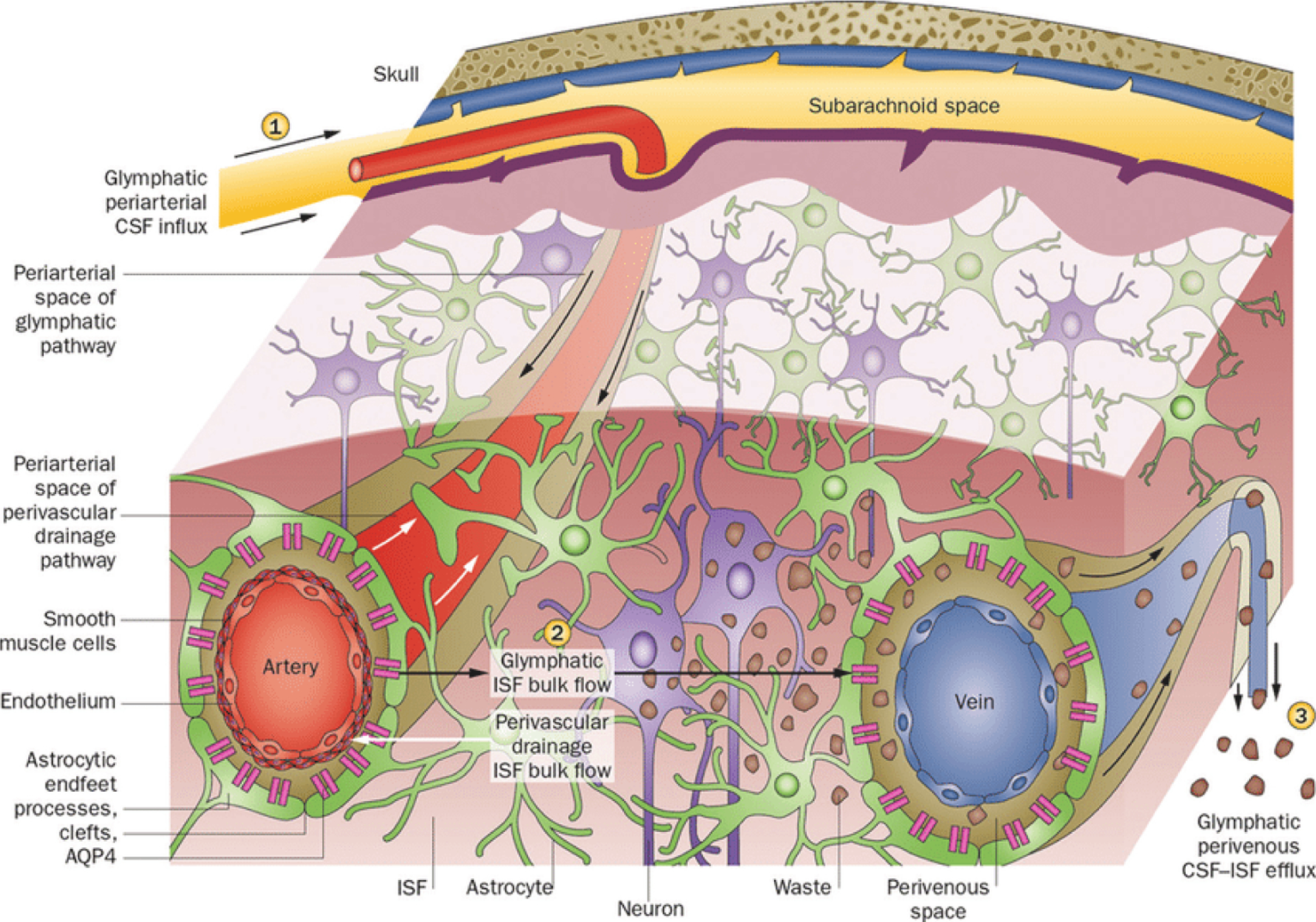
Outline of the glymphatic system. (1) Cerebrospinal fluid (CSF) flows into the brain parenchyma via the periarterial space, which is the perivascular space surrounding the parenchymal arteries. From this perivascular space surrounding the artery, CSF enters the interstitium of the brain tissue via aquaporin 4 (AQP4)-controlled water channels. These are distributed in the end feet of astrocytes that constitute the outer wall of the perivascular space. (2) Cerebrospinal fluid entering the interstitial fluid flows by convection, and the cerebral spinal fluid (CSF)-interstitial fluid (ISF) exchange within the brain parenchyma. (3) After washing the waste proteins from the tissue, it flows into the perivenous space, which is the perivascular space around the deep-draining vein and is subsequently discharged outside the brain. (Reprinted by permission from Macmillan Publishers Ltd: Nat Rev Neurol [11:457–470], copyright [2015]).

Despite recent advances in imaging and experimental techniques^9–11, a unified physiologically realistic and biomechanically rigorous brain-wide model of glymphatic transport that can provide a mechanistic understanding of the experimental observations is lacking (readers are referred to the review paper by Bohr et al¹² for an overview of existing models addressing different aspects and parts of the glymphatic system). Because of the complexity of the brain, the vast majority of previous models developed for glymphatic transport^13–18 were exclusively concerned with idealized material properties and geometries. Many of these models require a micro level of detail¹⁶, which is impractical to scale to the larger brain volumes necessary to evaluate macro level and subject-specific accounting of glymphatic function. This has potentially led to conflicting conclusions^13–16,19 where some have argued that glymphatic solute transport does not require convective flow since according to their simulations, arterial pulsation is unlikely to function as the driving force. Others have contended that interstitial transport may occur by both diffusion and convection where both mechanisms could be potentially relevant, thus comporting with strong experimental evidence that transport along the perivascular space is faster than diffusion. Further investigation of the effect of bulk CSF flow is warranted, particularly its relevance to the transport of molecules and agglomerates¹².

In-vivo imaging experiments have shown that CSF flow near arterial bifurcations is slow and complex with flow reversal present. These bifurcations appear to be common sites of Aβ accumulation in AD and a slow and oscillating flow might promote their deposition³. Thus, realistic 3D geometry is a prerequisite to creating physiological CSF flow and transport features necessary for accurately describing glymphatic function within the entire brain. Data-driven techniques, which combine brain-wide image-based measurements (e.g., MRI) with subject-specific computational models, have previously been utilized to estimate solute transport parameters that are difficult to measure including effective isotropic diffusivity^20,21, advective velocity magnitude field²² and local clearance²². This typically involves solving an optimization problem or an inverse problem with respect to image data. In this work, the main objective is to develop an image-informed 3D modeling framework to describe glymphatic transport and deposition of molecules, proteins, and nanoparticles in the entire brain where transport parameters are inferred directly from 3D imaging data, resulting in a flexible subject-specific model that accounts for anatomical geometry and heterogeneous material properties. This will enable us to gain predictive insights into the interplay between glymphatic dysfunction and protein deposition and provide a quantitative understanding of the underlying transport processes that render some brain regions more susceptible to protein deposits than others.

We have developed a coupled transport-damage model of glymphatic transport and amyloid accumulation that is solved using an immersed finite element method within an isogeometric analysis framework²³. By employing isogeometric analysis methodologies, we can obtain superior accuracy and robustness of the discretization compared with traditional finite elements. With an immersed method, we can avoid extensive and expensive segmentation that is required to construct geometry conforming meshes of the complex glymphatic pathways. In the approach, our model embeds the brain inside a simple non-conforming mesh aligned with the image volume bounding box, and the glymphatic pathways throughout the brain are modeled through the heterogeneity of the material property fields. Although in a boundary conforming setting, image-informed advection-diffusion model has been used to predict Rhenium-186 (¹⁸⁶Re)-nanoliposome distribution within the brain²⁴. While immersed methods have been used in other contexts including the analysis of trabecular bone^25–27, coated metal foam²⁷ and additive manufacturing²⁸, to our knowledge, this is the first time an image-informed immersed approach has been adopted for modeling 3D transport of molecules, agglomerates and debris within a brain.

The paper is organized as follows. Section 2 describes the mathematical models developed and methods applied. The results obtained from simulating an example case are presented in Section 3, followed by a discussion in Section 4.

2. Image-guided Glymphatic Transport Model

In this section, we propose a coupled model for the transport and deposition of amyloid throughout the entire brain. Then, we describe how a subject-specific model is constructed from image data. Finally, we present the numerical framework used to perform the simulation.

2.1. Model Definition

Let $\mathrm{\Omega }$ be the volume of a brain, and $\partial \mathrm{\Omega }$ its boundary. The boundary of the brain is decomposed into two mutually exclusive sets, $\partial \mathrm{\Omega }={\mathrm{\Gamma }}_R\cup {\mathrm{\Gamma }}_N$, where ${\mathrm{\Gamma }}_N$ is the portion of the boundary touching the skull, and ${\mathrm{\Gamma }}_R$ is the portion over which $\text{A}\beta$ is drained from the brain. $\text{A}\beta$ oligomers are soluble and can transport in the interstitial space. However, when they are fibrilized, they assemble into insoluble fibers and form $\text{A}\beta$ plaques that are resistant to degradation²⁹. We denote the concentrations of $\text{A}\beta$ or “soluble amyloid” by $c$ and amyloid plaque or “plaque” by $P$ in nM, where nM is nanomolar concentration. Glymphatic transport is modeled by the following equation.

$$\frac{\partial c}{\partial t}=\mathit{\nabla }\cdot (D\mathit{\nabla }c)-\mathit{\nabla }\cdot \left(c\mathit{u}\right)+S^{+}-\frac{\partial P}{\partial t}\mathrm{ } \text{in} \mathrm{\Omega }$$ (1)

The partial differential equation (PDE) in (1) is an advection-diffusion equation³⁰. $D$ is the diffusivity of soluble amyloid molecules in mm²/min, $\mathit{u}$ is the CSF velocity vector in mm/min, and $S^{+}$ is a volumetric source term that represents the production rate of soluble amyloid due to neural activity in nM/min. The last term in Eq.(1) models plaque deposition by allowing for soluble amyloid to agglomerate and convert to amyloid plaque. This term couples the transport model to an irreversible damage model for plaque accumulation³¹. The concentration of amyloid plaque is given by:

$$P\left(c\right)=\theta G\left(r\right(c\left)\right)$$ (2)

where $\theta$ is the amyloid plaque carrying capacity in nM, and $G$ is the plaque accumulation function. We assume that plaque deposition is initiated when the plaque accumulation parameter, $r$, exceeds a threshold, $r_i$ , and saturates when it reaches a threshold, $r_s$. This is modeled by choosing $G$ to be a smooth-step function defined in Eq. (2) (see Fig.2).

Fig. 2:

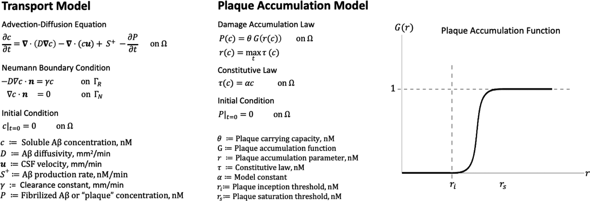
An overview of the mathematical model. The transport and deposition of $\text{A}\beta$ are modeled using an advection-diffusion equation coupled to a plaque accumulation model. Production and elimination of $\mathrm{A}\beta$ is accounted for by the source term, $S^{+}$ and the Robin boundary condition in the transport model, respectively. Amyloid plaque formation is an irreversible process that depends on the entire time history of the soluble amyloid concentration through the plaque accumulation parameter, $r$. Initially, we assume that plaque formation depends only on the soluble $\mathrm{A}\beta$ concentration through a constitutive model, $\tau =\alpha c$. We modeled amyloid plaque accumulation by a smooth step function $G\left(r\right)$, parameterized in terms of an inception threshold, $r_i$, which determines the critical point at which amyloid plaque begins to accumulate, and a saturation threshold, $r_S$, which determines the point at which no more amyloid plaque can be accumulated. Here, nM is nanomolar concentration.

$$G(\hat{r}(c))\mathrm{ }=\left\{\begin{array}{cc}0& r<r_i\\ 3\hat{r}(c{)}^2-2\hat{r}(c{)}^3,& r_i\le r\le r_s\\ 1& r>r_s\end{array}\right.$$ (3a)

$$\begin{array}{rr}& \\ \hat{r}\left(c\right)& =\frac{r\left(c\right)-r_i}{r_s-r_i}\end{array}$$ (3b)

The plaque accumulation parameter, $r$, depends on the complete time history of a constitutive law, $\tau$, that relates the concentration of soluble amyloid to the plaque accumulation parameter as follows.

$$r(c(\mathit{x},t))=\underset{s\in [0,t]}{\mathrm{m}\mathrm{a}\mathrm{x}}\tau (c(\mathit{x},s))$$ (4)

Defining the plaque accumulation parameter in this way ensures that given two time points, $t_0$ and $t_1$, the following holds.

$$t_0<t_1\Rightarrow P\left(\mathit{x},t_0\right)\le P\left(\mathit{x},t_1\right)$$ (5)

This can be verified by observing that $G$ is a non-decreasing function. Physically, this means that plaque deposition is modeled as an irreversible process. In this work, we assume $\tau$ is proportional to $c$,

$$\tau \left(c\right)=\alpha c,$$ (6)

where $\alpha$ is a model constant.

We also require that $c$ satisfies the following boundary conditions:

$$-D\mathit{\nabla }c\cdot \mathit{n}=\gamma c \text{on} {\mathrm{\Gamma }}_R$$ (7a)

$$\mathit{\nabla }c\cdot \mathit{n}=0 \text{on} {\mathrm{\Gamma }}_N$$ (7b)

where $\mathit{n}$ is the outward unit normal vector on ${\mathrm{\Gamma }}_R$ and ${\mathrm{\Gamma }}_N$. These boundary conditions model macro level features of glymphatic transport. The Robin type boundary condition in Eq. (7a) accounts for soluble amyloid cleared from the brain through the glymphatic drainage pathways within the subarachnoid space and dural lymphatic system. We assume that the diffusive flux of soluble amyloid leaving the boundary ${\mathrm{\Gamma }}_R$ is proportional to its concentration at the boundary. Here, $\gamma$ is the amyloid clearance parameter in mm/min. The larger the clearance parameter, the more “efficiently” a given concentration of soluble amyloid is cleared. The homogeneous Neumann boundary condition in Eq. (7b) is an impenetrability constraint which prevents amyloid from leaving the skull on ${\mathrm{\Gamma }}_N$. Violation of this condition would lead to physical inconsistencies in the model. Finally, we specify initial conditions for $c$ and $P$ , given in Eq. (8).

$${\left.c\right|}_{t=0}=0$$ (8a)

$${\left.P\right|}_{t=0}=0$$ (8b)

That is, the system begins with no soluble amyloid or amyloid plaque in $\mathrm{\Omega }$.

2.2. Subject-Specific Model Construction

In order to construct a subject-specific model for glymphatic transport, we infer the model geometry and parameters from diffusion-weighted MRI (DW-MRI) data. To create the geometry, we segment the brain volume, $\mathrm{\Omega }$, from the MR image volume (Fig.3). This is done automatically by thresholding the MR image voxel intensities to a value greater than zero. After the volume is obtained, the boundary, $\partial \mathrm{\Omega }$, is manually segmented as belonging to the skull or drainage points to partition $\partial \mathrm{\Omega }$ into ${\mathrm{\Gamma }}_R$ and ${\mathrm{\Gamma }}_N$, respectively. For the mouse brain, ${\mathrm{\Gamma }}_R$ is defined along the inferior and posterior regions of the brain near the Circle of Willis and dural lymphatic pathways shown to play a strong role in CSF clearance from the brain³² (Fig.3). Assuming that the diffusivity of amyloid molecules can be approximated by that of water molecules, an apparent diffusion coefficient (ADC) map derived from the DW-MRI data can be used for the diffusivity coefficient, $D$. The CSF-flow velocity vector field can be inferred from contrast-enhanced(CE)-MRI data. The velocity vector field values are constrained to satisfy the following no-slip boundary condition.

Fig. 3:

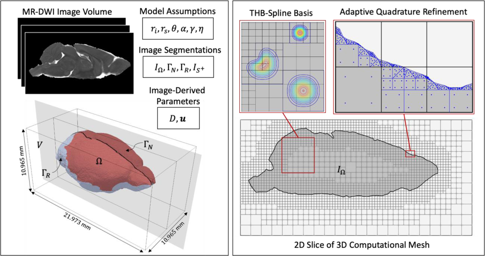
An overview of the image-guided 3D model construction and computational framework. The left panel shows the model inputs. These include (i) image data; (ii) image segmentations, where a binary labelmap, $I_{\mathrm{\Omega }}$ , is segmented from the image volume, $V$ , to isolate the region, $\mathrm{\Omega }\subset V$ , occupied by the subject’s brain and the boundary of $\mathrm{\Omega }$ is segmented into two sets, ${\mathrm{\Gamma }}_R$ and ${\mathrm{\Gamma }}_N$, in order to define where to apply the appropriate boundary conditions; (iii) model parameters that come from image data, $D$ and $\mathbf{u}$; (iv) model parameters that are assumed, namely $r_i,r_s,\theta ,\alpha ,\gamma$ , and $\eta$. The right panel shows details about the analysis. A 3D computational mesh aligned to $V$ is constructed. The mid-sagittal plane of the 3D mesh is shown here. We use a quadratic THB-spline discretization of $c$ with adaptive refinement on $\partial \mathrm{\Omega }$. For integration, an adaptive quadrature rule is utilized that uses the brain segmentation, $I_{\mathrm{\Omega }}$, to adaptively subdivide and tessellate the cut elements. Here, four levels of quadrature refinement are shown. After trimming and basis removal, the number of elements used is 35,639 and the total degrees of freedom for $c$ is 41,618.

$$\mathit{u}=\mathbf{0} \text{on} \partial \mathrm{\Omega }$$ (9)

The $\text{A}\beta$ peptide is produced through cleaving of the amyloid precursor protein (APP), which is a membrane protein found in many tissues, particularly neurons²⁹. For this model, we assume that soluble amyloid production sites correlate with prominent white matter tracts that are composed of neuronal axonal fibers, while other regions such as gray matter are composed of dendrites and nerve cell bodies. Since white matter regions that contain prominent tracts of neurons are more anisotropic than other regions of the brain³³, we segment these regions from the DW-MRI data through thresholding of fractional anisotropy (FA) values between 0.3 and 1.0. The segmentation is used to define an indicator function $I_{S^{+}}$ that is equal to 1 within the prominent white matter tracts and 0 elsewhere. The amyloid source term is then defined as $S^{+}=\eta I_{S^{+}}$, where $\eta$ is the $\mathrm{A}\beta$ production rate with a unit of nM/min.

In general, $D,\mathit{u}$ , and $S^{+}$ may vary over time. CSF velocity described by $\mathit{u}$ is tied to the cardiac cycle (seconds) and is described through both bulk and pulsatile flow³⁴. Using a time series of image data, it is possible to create temporal interpolations of these spatially varying fields³⁵. Since we are interested in simulating macro level glymphatic transport and amyloid plaque accumulation that occurs over long periods of time (months), we consider time averages of these fields in this work. Therefore, we let $D,\mathit{u}$, and $S^{+}$ remain constant over time. Note, the image derived parameters $D,\mathit{u}$, and $S^{+}$ are all smoothed using a projection method³⁶.

The remaining model parameters, namely $r_i,r_S,\theta$ and $\alpha$, are constants that are part of the plaque accumulation model. Discrete values for initial and saturation concentration threshold of amyloid for plaque buildup cover wide ranges depending on experimental parameters (e.g., in vitro, in vivo, domain size, model organism, etc.). As a first approximation, we assume nominal values of these parameters (see Table 1) informed through common literature values that matched expected concentrations in a mouse model of amyloid buildup^37–39. In the future, these parameters are to be calibrated according to experimental data in order to maximize correlation between the model predictions and experimental results.

Table 1:

Model parameters used in simulation

Plaque accumulation model parameters	Value	Source
Plaque inception threshold, $r_i$	10,000 nM*	Hu et al.37 / Raskatov et al.38
Plaque saturation threshold, $r_s$	50,000 nM	Raskatov et al.38
Plaque carrying capacity, $\theta$	50,000 nM	Raskatov et al.38
Constitutive model constant, $\alpha$	1	—
Transport model parameters
CSF flow velocity (nominal), $u_0$	4.2 mm/min	†Li et al.39
Soluble $\mathrm{A}\beta$ production rate, ${\eta }_0$	0.2 nM/min	Raskatov et al.38
Clearance constant, ${\gamma }_0$	0.00002 mm/min	See note below‡

^*nM = Nanomolar concentration

^†Literature sources of brain-wide measures of CSF velocity are difficult given the very large discrepancy between ventricular CSF flow and flow in perivascular spaces or other brain parenchymal regions. Phase-contrast(PC)-MRI methods, in particular, have reported higher estimates of CSF velocity than other methods. While PC-MRI methods are attractive for parameterization since we are using MRI data for this model, we chose our nominal value (70 um/s or 4.2 mm/min) to be closer to in situ and flow-based measures³⁹ rather than PC-MRI estimates since our DWI estimates within fluid-filled spaces such as the ventricles would not scale in the same manner as phase-contrast methods.

^‡This nominal value γ₀ was selected based on a 0-D approximation of the system behavior that yields a steady-state solution equal to the inception threshold: c = 10,000 nM.

2.3. Numerical implementation

In this section, we provide details on the numerical implementation for solving the glymphatic transport model. We begin by introducing notation for a residual, $R$, by rewriting Eq. (1) as follows.

$$\begin{gathered} R\left(c\left(\mathit{x},t\right)\right):=\frac{\partial c\left(\mathit{x},t\right)}{\partial t}+\frac{\partial P\left(c\left(\mathit{x},t\right)\right)}{\partial t}-\mathit{\nabla }\cdot \left(D\left(\mathit{x}\right)\mathit{\nabla }c\left(\mathit{x},t\right)\right)+\mathit{\nabla }\cdot \left(c\left(\mathit{x},t\right)\mathit{u}\left(\mathit{x}\right)\right) \\ -S^{+}\left(\mathit{x}\right)=0 \end{gathered}$$ (10)

For clarity, we have explicitly noted the spatial and temporal dependence for each variable. The strong form of the glymphatic transport problem is summarized by Eqs. (1), (7) and (8). The weak form of the problem with Streamline upwind Petrov-Galerkin (SUPG) stabilization is to find $c\in H^1\left(\mathrm{\Omega }\right)$ such that $\forall w\in H^1\left(\mathrm{\Omega }\right)$ the following holds.

$$\begin{gathered} \frac{d}{dt}{\int }_{\mathrm{\Omega }}wcdx+\frac{d}{dt}{\int }_{\mathrm{\Omega }}wPdx+{\int }_{\mathrm{\Omega }}D\mathit{\nabla }c\cdot \mathit{\nabla }wdx-{\int }_{\mathrm{\Omega }}c\mathit{u}\cdot \mathit{\nabla }wdx+{\int }_{{\mathrm{\Gamma }}_R}\gamma wcd\mathrm{\Gamma } \\ \mathrm{ }-{\int }_{\mathrm{\Omega }}w{S}^{+}dx+{\int }_{\mathrm{\Omega }}\sigma R\left(c\right)\mathit{u}\cdot \mathit{\nabla }wdx=0 \end{gathered}$$ (11)

In (11), $\sigma$ is the stabilization parameter, $h$ is a characteristic length for the mesh element size, and $P{e}^h$ is the element Peclet number. Note, the Neumann boundary conditions in Eqs. 7a and 7b are imposed weakly, and therefore become a part of the weak form in Eq. 11.

$$\sigma =\frac{h}{2\left|\mathit{u}\right|}\mathrm{m}\mathrm{i}\mathrm{n}\left(\frac{P{e}^h}{3},1\right)$$ (12)

$$\begin{array}{rr}& \\ P{e}^h& \mathrm{ }=\frac{\left|\mathit{u}\right|h}{2D}\end{array}$$ (13)

Given a time interval [0, T] under consideration, we pick out uniformly spaced time steps $\left\{t_0=0,t_1,t_2,\cdots ,t_N=T\right\}$ and use a superscript to indicate the particular time step at which a quantity is being evaluated i.e. $v^n:=v\left(t_n\right)$. The uniform time interval used to define these time steps is denoted by $\mathit{\Delta }t$. With these definitions, we set out to use the backward Euler scheme to discretize the weak form (11) in time. Given $c^n$ and $P^n$, we solve for $c^{n+1}$ and $P^{n+1}$ using the following equation.

$$\begin{gathered} {\int }_{\mathrm{\Omega }}w\frac{c^{n+1}-c^n}{\mathit{\Delta }t}dx+{\int }_{\mathrm{\Omega }}w\frac{P^{n+1}-P^n}{\mathit{\Delta }t}dx+{\int }_{\mathrm{\Omega }}D\mathit{\nabla }{c}^{n+1}\cdot \mathit{\nabla }wdx \\ +{\int }_{{\mathrm{\Gamma }}_R}\gamma w{c}^{n+1}d\mathrm{\Gamma }-{\int }_{\mathrm{\Omega }}{c}^{n+1}\mathit{u}\cdot \mathit{\nabla }wdx-{\int }_{\mathrm{\Omega }}w{\left(S^{+}\right)}^{n+1}dx \\ +{\int }_{\mathrm{\Omega }}\sigma R\left(c^{n+1}\right)\mathit{u}\cdot \mathit{\nabla }wdx=0 \end{gathered}$$ (14)

In order to obtain a discrete system of equations from (14) which we can solve numerically, we make use of an immersed finite element method²⁷. Let $V$ denote the entire MR image volume. Since $\mathrm{\Omega }\subset V$, we can create an extension of the problem from $\mathrm{\Omega }$ to $V$ by introducing an indicator function, $I_{\mathrm{\Omega }}$.

$$I_{\mathrm{\Omega }}=\left\{\begin{array}{ll}1,& \text{in} \mathrm{\Omega }\\ 0,& \text{in} V-\mathrm{\Omega }\end{array}\right.$$ (15)

$I_{\mathrm{\Omega }}$ is constructed directly from the brain volume labelmap segmentation. The weak form is then transformed in terms of integration over the image volume.

$$\begin{gathered} {\int }_V{I}_{\mathit{\Omega }}w\frac{c^{n+1}-c^n}{\mathit{\Delta }t}dx+{\int }_V{I}_{\mathit{\Omega }}w\frac{P^{n+1}-P^n}{\mathit{\Delta }t}dx+{\int }_V{I}_{\mathit{\Omega }}D\mathit{\nabla }{c}^{n+1}\cdot \mathit{\nabla }wdx \\ -{\int }_V{I}_{\mathit{\Omega }}{c}^{n+1}\mathit{u}\cdot \mathit{\nabla }wdx-{\int }_V{I}_{\mathit{\Omega }}w{\left(S^{+}\right)}^{n+1}dx \\ +{\int }_V{I}_{\mathit{\Omega }}\sigma R\left(c^{n+1}\right)\mathit{u}\cdot \mathit{\nabla }wdx+{\int }_{{\mathrm{\Gamma }}_R}\gamma w{c}^{n+1}d\mathrm{\Gamma }=0 \end{gathered}$$ (16)

This immersed formulation introduces a discontinuity in the integrands which is rectified using a quadrature rule with adaptive refinement on $\partial \Omega$ ²⁵. The adaptive refinement is carried out in two steps: starting from the base mesh, 1) elements intersecting $\partial \mathrm{\Omega }$ are subdivided $n$ times, and then 2) a triangulation of the subdivided elements intersecting $\partial \mathrm{\Omega }$ (Fig.3).

The immersed approach also allows the discretization of $c$ and $P$ to be constructed from a mesh on $V$ as opposed to a boundary conforming mesh in $\mathrm{\Omega }$. This has practical benefits in terms of mesh construction and creating a smooth discretization.

The concentrations $c$ and $P$ are approximated using a finite-dimensional space $W^h\subset H^1\left(V\right)$ which is made up of degree two THB-splines^40,41 obtained from a hierarchical mesh aligned with $V$ (Fig.3). Any basis functions with no support in $\mathrm{\Omega }$ are removed from the discretization. Let $\left\{N_i\left(x\right)\right\}$ denote such a basis. Then, we can approximate $c$ in terms of unknown degrees of freedom, $\left\{c_i\right\}$.

$$c\approx c_h=\sum _i{c}_i\left(t\right)N_i\left(x\right)$$ (17)

This transforms into a matrix-vector problem we can solve numerically. We define the following operators.

$$H_{ij}:={\int }_{{\mathrm{\Gamma }}_R}\gamma N_i{N}_{j}d\mathrm{\Gamma }$$ (18)

$$M_{ij}:={\int }_V{I}_{\mathrm{\Omega }}{N}_i{N}_{j}dx+{\int }_V{I}_{\mathrm{\Omega }}\left(\sigma \mathit{u}\cdot \mathit{\nabla }{N}_i\right)N_{j}dx.$$ (19)

$$K_{ij}:={\int }_V{I}_{\mathrm{\Omega }}D\mathit{\nabla }{N}_i\cdot \mathit{\nabla }{N}_{j}dx+{\int }_V{I}_{\mathrm{\Omega }}\mathit{\nabla }\cdot \left(D\mathit{\nabla }{N}_j\right)\left(\sigma \mathit{u}\cdot \mathit{\nabla }{N}_i\right)dx$$ (20)

$${\text{A}}_{ij}:={\int }_V{I}_{\mathrm{\Omega }}\left(\mathit{u}\cdot \mathit{\nabla }{N}_i\right)N_{j}dx+{\int }_V{I}_{\mathrm{\Omega }}\left(\sigma \mathit{u}\cdot \mathit{\nabla }{N}_i\right)\mathit{\nabla }\cdot \left(\mathit{u}{N}_j\right)dx$$ (21)

$$b_i:={\int }_V{I}_{\mathrm{\Omega }}{S}^{+}{N}_{i}dx+{\int }_V{I}_{\mathrm{\Omega }}{S}^{+}\left(\sigma \mathit{u}\cdot \mathit{\nabla }{N}_i\right)dx$$ (22)

$$L\left(c_j^{n+1}\right):=M_{ij}{c}_j^{n+1}+\Delta t\left[K_{ij}-{\text{A}}_{ij}+H_{ij}\right]c_j^{n+1}$$ (23)

$$d_i:={\int }_V\left(P\left(c^{n+1}\right)-P\left(c^n\right)\right)N_i$$ (24)

Using these definitions, the discretized weak form is expressed as follows.

$$L\left(c_j^{n+1}\right)=M_{ij}{c}_j^n-d_i+\Delta t{b}_i$$ (25)

The system of equations in (26) are nonlinear in $c^{n+1}$ due to the function $G$ that appears in the damage model. In order to obtain a solution, we use a fixed-point iteration scheme.

Computations were carried out in Nutils⁴², an open source finite element Python library.

3. A 3D model of glymphatic transport in a mouse brain

Key inputs informing the glymphatic transport model are subject-specific brain anatomy, CSF velocity in the glymphatic pathway, and diffusivity of molecules, proteins, and debris throughout the brain. The material property diffusivity for $\text{A}\beta$ molecules is inferred directly from a set of DW-MRI data of C57BL/6 mouse brain publicly accessible from the Duke University Center for In Vivo Microscopy⁴³ (Fig. 4A). While the CSF velocity field can be obtained from CE-MRI data of a mouse brain, no direct measures of velocity are available for this publicly available mouse brain dataset. Therefore, as an initial approximation, the CSF velocity field (Fig. 4B) is simulated from the available DW-MRI data (see Appendix for details). The spatial distribution of $\text{A}\beta$ sources (Fig. 4C) was determined by identifying prominent white matter regions as localized “sources” for $\text{A}\beta$ through thresholding of higher diffusivity values and anatomical co-registration (see Appendix). Material properties at each image voxel are converted into an analysis suitable function for simulation purposes using projection methods. Table 1 lists the parameter values used in the simulations. The resulting 3D distribution of soluble amyloid is shown in Fig. 4D.

Fig. 4:

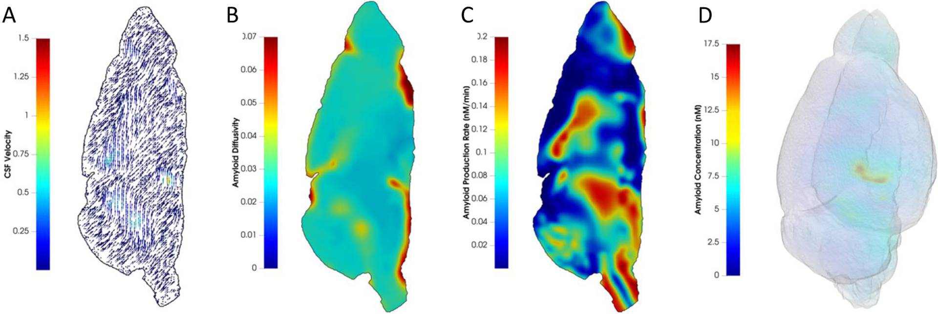
Spatial distribution of model input parameters and resulting soluble amyloid distribution. (A) CSF velocity vector field colored with velocity magnitude in mm/min; (B) apparent diffusion coefficient in mm²/min; (C) amyloid production rate in nM/min; and (D) A 3D view of the concentration of soluble amyloid beta in nM at $t=60$ minutes. Here, nM indicates nanomolar concentration.

Two experimental states are tested with this model: 1) a short-term, thirty-minute simulation study of soluble amyloid accumulation, and 2) a long-term simulation study of soluble amyloid and eventual plaque development over 12 months. In the short-term study, we compare glymphatic transport simulation results to published data from Gaberel et al.¹⁰ who performed dynamic contrast enhanced (DCE)-MRI studies with gadolinium (Gd) tracer, and used that to determine CSF flow and resulting Gd accumulation as part of their experiments. In the simulation, we use a time step of 5 mins, 2 levels of mesh refinement, and 4 levels of quadrature refinement. These early time-point results are encouraging in that we demonstrate similar geometry of CSF-embedded tracer distribution matching CSF-embedded Gd signal enhancement in¹⁰ (Fig.5). In the long-term study, the time course of soluble amyloid accumulation and resulting plaque deposition is simulated within the mouse brain. In the simulation, we use and a time step of 60 mins, 2 levels of mesh refinement and 2 levels of quadrature refinement and a single fixed-point iteration scheme to approximate the numerical solution. In Fig.6, we report soluble amyloid concentration normalized by the total soluble amyloid produced per unit volume within the domain over 12 months and plaque concentration normalized by the plaque carrying capacity, $\theta$. Plaque deposition pattern is strongly influenced by that of soluble amyloid concentration. Both soluble amyloid and amyloid plaque preferentially accumulate toward the anterior region of the brain in much higher concentrations than any other brain region, even as early as 2 months into the simulation. The anterior regions appear saturated with plaque as the long-term study approaches 12 months. This preferential buildup of plaque is largely because CSF flow velocity vectors are predominantly directed toward the brain anterior (Fig. 4A) which drives the soluble amyloid toward that region causing its concentration to increase rapidly with time.

Fig. 5:

A qualitative comparison of simulation results with experimental data. (A) Time course of DCE-MRI studies showing Gd accumulation over 30 minutes within a mouse brain (reprinted by permission from Wolters Kluwer Health, Inc.: Stroke [45 (10):3092–3096], copyright [2014]). (B) Time course of soluble amyloid accumulation over 30 minutes within a mouse brain. The mid-sagittal plane is shown.

Fig. 6:

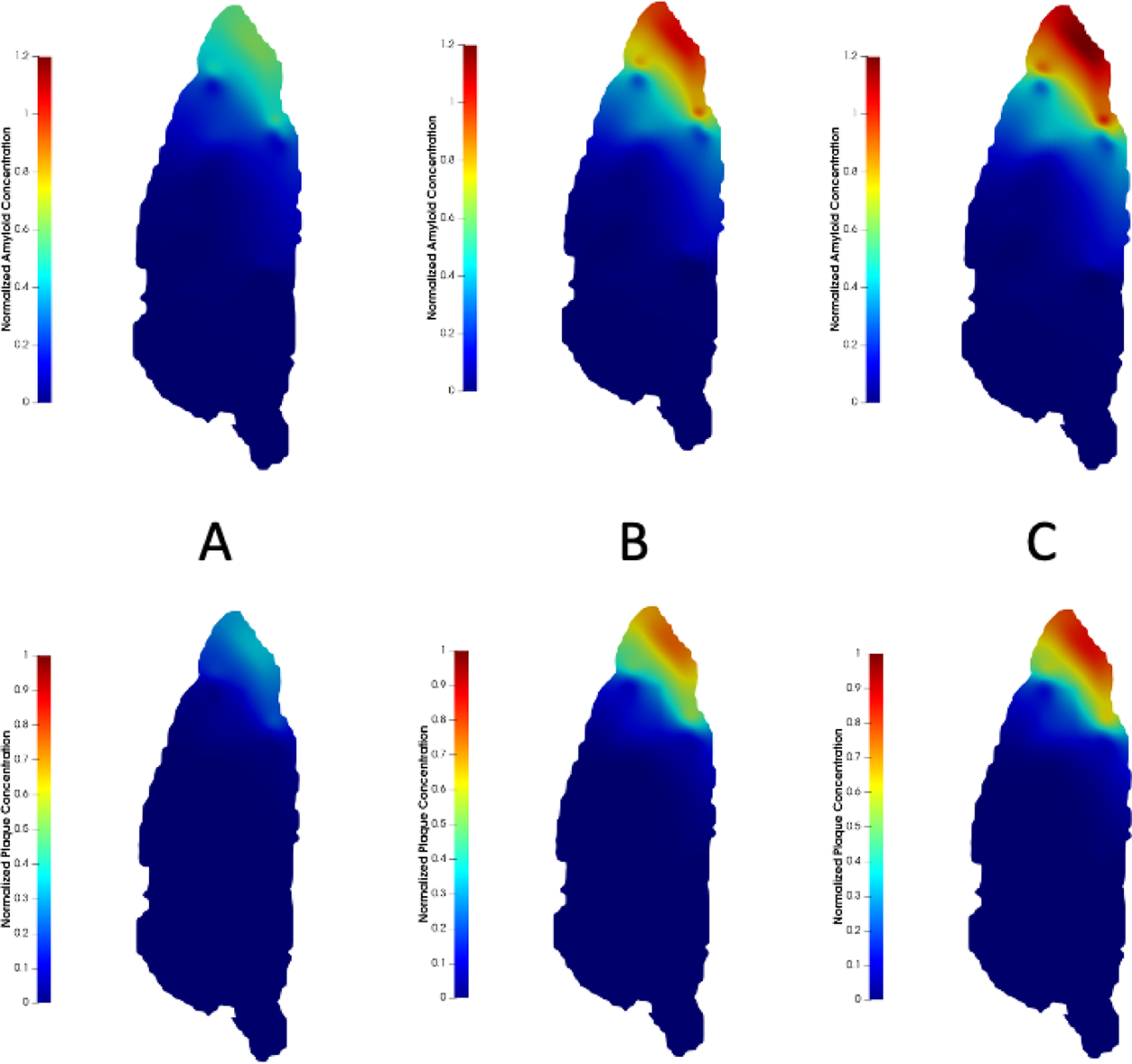
Soluble amyloid and amyloid plaque distribution at (A) $t=2$ months; (B) $t=7$ months; and (C) $t=12$ months. Top row: soluble amyloid concentration is normalized by the total soluble amyloid produced per unit volume within the domain over 12 months. Bottom row: amyloid plaque concentration is normalized by the plaque carrying capacity $\theta$. The mid-sagittal plane is shown.

To further investigate this sharp development of plaque in the anterior region, we considered total soluble amyloid and plaque within the domain (Fig.7). We note a bi-phasic behavior for plaque accumulation. Plaque deposition appears to start in the first month and it rapidly builds up initially until month 7, after which the rate of plaque accumulation decreases and slowly plateaus. Between month 7 and month 12, less plaque is formed. Similarly, total soluble amyloid content within the brain increases rapidly in the early stages until month 4 before approaching a plateau around month 10. As the concentration of amyloid throughout the domain increases with time, the amount of soluble amyloid available for clearance at the boundary also increases. This causes amyloid clearance rate, defined as the amount of soluble amyloid cleared through the boundary per unit time, to increase with time (Fig.8). Thus, with the rate of soluble amyloid introduced into the domain remaining constant over time, less soluble amyloid is available to form amyloid plaque. As a result, the rate of plaque deposited decreases over time.

Fig. 7:

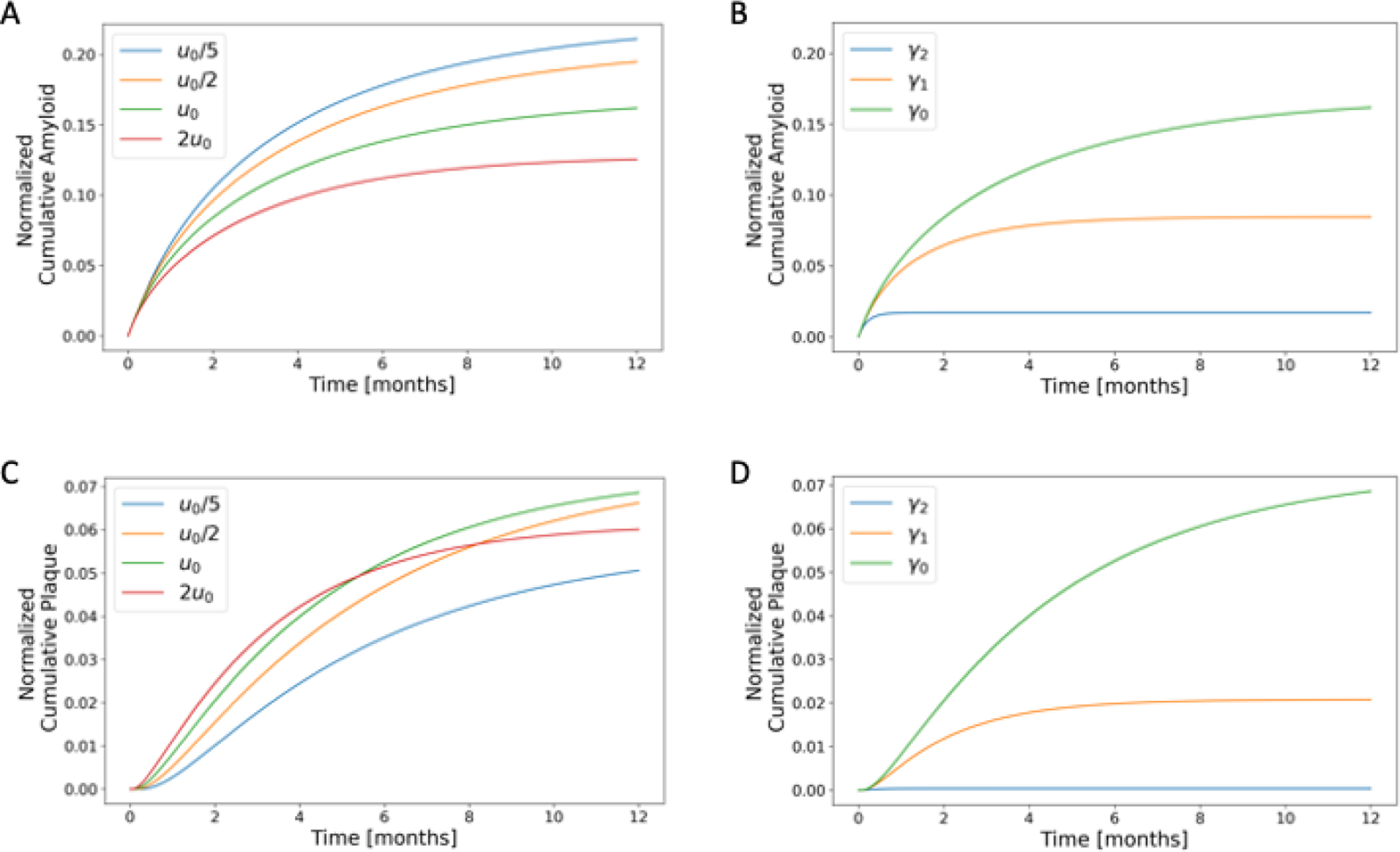
A parametric study of the effect of CSF flow velocity and clearance constant on glymphatic transport and amyloid deposition. (A) and (B) show time evolution of total (cumulative) soluble amyloid content in the domain normalized by total amyloid introduced to the domain over a 12-month period. (C) and (D) show time evolution of total (cumulative) amyloid plaque deposited normalized by maximum possible amyloid plaque accumulation in the domain. CSF flow cases considered in (A) and (C) are: “slowest” ($\left.u_0/5\right)$ in blue; “slower” $\left(u_0/2\right)$ in orange; “nominal” $\left(u_0\right)$ in green; and “faster” $\left(2u_0\right)$ in red. Clearance constant cases considered in (B) and (D) are: ${\gamma }_0;{\gamma }_1=2{\gamma }_0$; and ${\gamma }_2=10{\gamma }_0$ , where ${\gamma }_0$ is the nominal value.

Fig. 8:

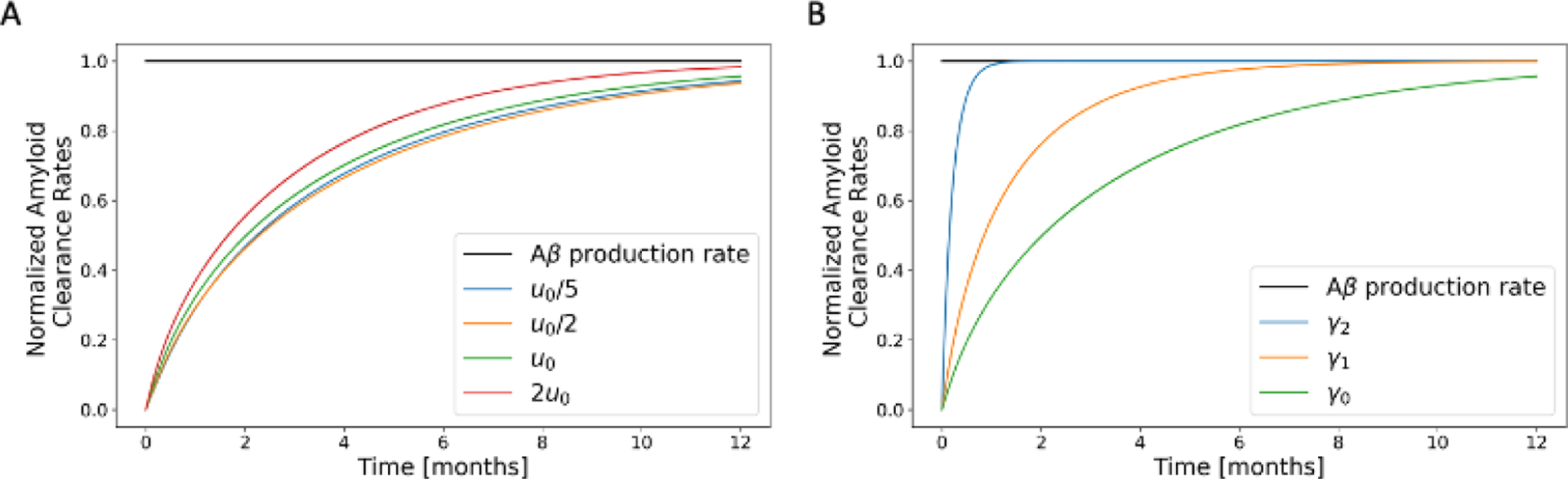
A parametric study of the effect of CSF flow velocity and clearance constant on amyloid clearance. Clearance rate of soluble amyloid from the brain is normalized by the rate at which soluble amyloid is produced in the brain over a 12-month period. CSF flow cases considered in (A) are: “slowest” $\left(u_0/5\right)$ in blue; “slower” $\left(u_0/2\right)$ in orange; “nominal” $\left(u_0\right)$ in green; and “faster” $\left(2u_0\right)$ in red. Clearance constants considered in (B) are: ${\gamma }_0;{\gamma }_1=2{\gamma }_0$; and ${\gamma }_2=10{\gamma }_0$ , where ${\gamma }_0$ is the nominal value.

We conducted a parametric study of the effect of CSF flow velocity on glymphatic transport and deposition of amyloid over 12 months (Fig.7). At early time points, plaque accumulates more rapidly for increased CSF flow velocities. However, these cases also reach steady state faster resulting in less plaque deposition over longer periods of time compared to slower CSF flow velocities. Under slower CSF flow conditions, a more diffused distribution of amyloid plaque is seen in the brain inferior region compared to faster CSF flow cases (Fig.9). A parametric study of the effect of the clearance constant, $\gamma$ , on glymphatic transport shows an increase in plaque accumulation with decreasing clearance constant (Fig.8).

Fig. 9:

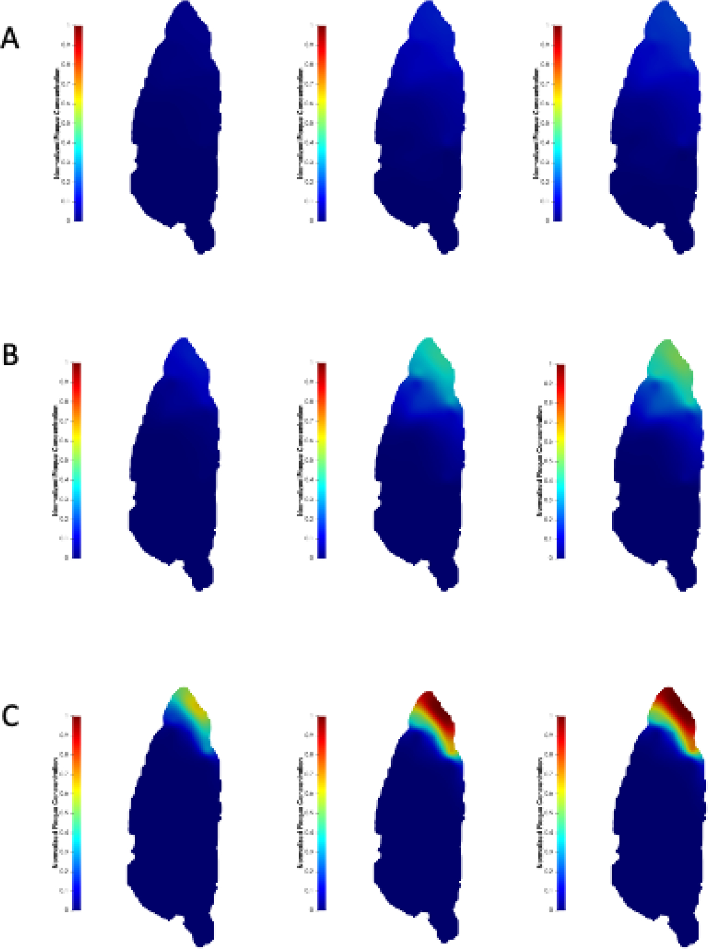
Effect of CSF flow velocity on amyloid deposition. Amyloid plaque concentration normalized by plaque carrying capacity $\theta$ at $t=2$ (left column), 7 (mid column) and 12 (right column) months for the (A) “slowest” ($\left.u_0/5\right)$); (B) “slower” ($\left.u_0/2\right)$); and (C)”faster” ($\left(2u_0\right)$) cases, compared to the “nominal” $\left(u_0\right)$ case. The mid-sagittal plane is shown.

4. Discussion

The methods of computational fluid dynamics (CFD) provide validated models of transport, which we have applied extensively to the cardiovascular system^30,44–48 and cerebrovascular system^49–51. As a logical extension of this approach, we modeled glymphatic transport, including both CSF flow and diffusion of biomarkers via the glymphatic pathway, in an integrated manner. The tight integration of the glymphatic transport model with image data in this framework provides a template for a subject-specific analysis with physiologically realistic parameters. Our approach is designed to maximize the utilization of information available through imaging techniques. This is done by incorporating the image-derived information as input parameters or constraints into the models. As new imaging data become available or the models are further validated, the process can be repeated to update and refine the models, leading to more accurate predictions or understanding. In contrast, previous methodologies use estimates that either depend on additional layers of modeling and approximation or rely on the model itself to establish a numerically valid range. In those cases, transport of $\text{A}\beta$ was investigated through micro-volumes of the brain^13–16. Instead of treating CSF velocity as a material property, it is either neglected or computed using a Darcy or Navier-Stokes flow model. This introduces additional material properties such as pressure, permeability, and influx/efflux conditions at the perivascular space boundaries¹⁶. Our approach, which infers the CSF flow field from image data rather than through CFD computation, avoids these issues because geometric features of the glymphatic pathways are implicitly represented through the variations of the imaged CSF flow field. Therefore, the importance of bulk flow in $\text{A}\beta$ transport, which has been debated throughout literature^13–16,19, is not a result of our modeling decisions, but rather dictated by the spatially varying material properties derived from subject-specific image data. For the deposition of $\text{A}\beta$, previous publications have presented compartmental models that attempt to describe the evolution and interaction between soluble and fibrilized $\text{A}\beta$ (amyloid plaque) throughout the brain⁵². These models use rate parameters. Even if experimentally derived, estimates of these rate parameters are typically valid only for a specific range of conditions or limited geometries. Our image-based modeling approach by design allows for a more subject-specific accounting of parameters from imaging data, thus paving the way for a more accurate modeling of transport and plaque deposition within the entire brain.

Associated with a subject-specific modeling framework for simulating glymphatic transport, is the challenge of accounting for the geometric features provided by the scanned images of the brain. In particular, the construction of computational meshes that conform to the geometric features of the scanned data, as is done with classical finite element and isogeometric methods, can be prohibitively cumbersome. To circumvent the complexity of boundary conforming mesh generation, we use so-called immersed methods where a tensor-product computational domain is created in which the image-based domain of interest is immersed. The advantage of such an immersed approach is clear: complicated meshing operations are avoided, and the image data is used to segment the computational tensor-product domain instead. However, the image-based segmentation introduces discontinuous functions that represent the immersed geometric features of the image/scan-based domain within the computational tensor-product mesh. Resolving and integrating such discontinuous functions requires mesh refinement and nonstandard quadrature rules that may lead to proliferation of computational complexity. By using THB-splines to generate the computational mesh, we are able to exploit local refinement strategies for efficient computations.

Our glymphatic transport simulation results in a mouse brain reflect similar tracer accumulation patterns seen in the short-term experiment, which is encouraging. The trends of the long-term simulation results indicate that plaque deposition increases with lower CSF flow velocity signifying glymphatic dysfunction and decreases with higher CSF flow velocity. These findings suggest that a threshold level of CSF velocity may exist below which amyloid plaque deposition occurs, and factors that enhance CSF flow (e.g., exercise) and promote glymphatic function may forestall neurodegenerative disease progression. The results of the clearance constant $\left(\gamma \right)$ parameter sweep indicate that an optimum value of $\gamma$ may exist for preventing plaque accumulation and that a decline in amyloid “clearance efficiency” resulting from age or disease progression can trigger amyloid plaque deposition.

However, long-term simulations fall short in capturing expected distribution pattern for amyloid plaque. Of note, the high concentration of soluble amyloid and resulting plaque development near the brain anterior. In many mouse models of AD, plaque deposits are seen throughout the brain, particularly in cortical and hippocampal regions of the midbrain⁵³. While plaques may also develop in the mouse brain anterior, the simulated concentration and speed of development do not match experimental results⁵⁴. One major parameter that may be causing this behavior is the CSF velocity field. Well-described, 3D fields of CSF velocity for the entire mouse brain are difficult to generate and usually confined to periods of up to 2 hours. CSF velocity fields in this simulation rely on DWI data parameters for scaling and are assigned preferential directions based on the observations of such studies. In long-term studies, however, the long-term dynamics of 3D CSF fluid are far more complex.

Discrepancies between simulated plaque accumulation results and experimental observations could also be attributed to the limitations and simplifying assumptions made in this model. Since plaque accumulation model parameters, namely $\theta ,r_i,r_s$ , and $\alpha$ are currently non-measurable, we relied on relevant literature values and justified their use based on trends observed in experiments. In addition, we do not consider boundary flow effects such as transport to and from the subarachnoid space and meninges, and soluble amyloid clearances are generally idealized near the brain inferior. Further, simulated CSF velocities do not reach the peak values reported by other sources. The model is also limited by the fact that time varying changes in velocity field were neglected, as we opted for a time-averaged velocity field due to lack of long-term data. Moreover, any changes in transport parameters due to aging and disease process are not considered either. However, few studies consider both magnitude and direction of CSF velocities, as we have done in this work.

Many of these challenges could be improved through parameterization with more accurate velocity fields from in vivo imaging data techniques such as DCE-MRI to match the DW-MRI data acquired on the same imaging field in the same animal. These techniques will also allow for characterization of changes in amyloid concentration across tissue boundaries, which will better inform our clearance modeling parameters. Planned future work therefore includes performing imaging studies in mouse models of amyloid build up⁵⁵ and wild-type controls at various ages to create subject-specific computational models. For estimation of non-measurable parameters $\theta ,r_i,r_s$ , and $\alpha$ in the plaque accumulation model, $\text{A}\beta$ production rate, $\eta$ , an inverse problem will be solved with respect to imaging data using methodologies described in⁵⁶. This will result in a well-validated computational toolset capable of quantitatively assessing the effect of glymphatic dysfunction on amyloid deposition and investigating how physiological factors such as exercise affect glymphatic transport.

In summary, given the numerous hypotheses⁵⁷ for the role that the glymphatic system plays in the pathogenesis of neurodegenerative disease, this work provides the necessary foundation for developing an architecturally and physiologically faithful 3D platform, grounded in experiments, to test these hypotheses, which will greatly assist in the development of future preventive and therapeutic interventions. In addition, our modeling framework lays the groundwork for future image-guided modeling of the human glymphatic transport, as creating subject-specific models using noninvasive MRI holds great potential for eventual clinical translation.

APPENDIX

A1. Derivation of a simulated CSF flow field from DW-MRI data

For our simulation, we require two input parameters, a velocity field with three components, $u_i$ , and diffusivity, $D$. This means that at each point in our simulation domain, we will have three orthogonal components of velocity: right-left (RL), anterior-posterior (AP), and superior-inferior (SI). We took DW-MRI data made publicly accessible from the Duke University Center for In Vivo Microscopy (CIVM)⁴³. From the CIVM dataset, the apparent diffusion coefficient (ADC) map serves as our diffusivity term. We generated velocity fields by first deriving the eigenvalues $\left({\lambda }_1,{\lambda }_2,{\lambda }_3\right)$ from DW-MRI dataset using the ADC and fractional anisotropy (FA) maps using the below equations²:

$$ADC=\frac{ \mathit{\text{Trace}} }{3}=\frac{{\lambda }_1+{\lambda }_2+{\lambda }_3}{3};F\text{A}=\sqrt{\frac{{\left({\lambda }_1-{\lambda }_2\right)}^2+{\left({\lambda }_2-{\lambda }_3\right)}^2+{\left({\lambda }_1-{\lambda }_3\right)}^2}{2\left({\lambda }_1^2+{\lambda }_2^2+{\lambda }_3^2\right)}}$$ (A1)

Once derived, we squared the trace and scaled that quantity to a velocity magnitude of ${\text{u}}_0=70\mathrm{ }\mu \mathrm{m}/\mathrm{s}$⁵⁸, and then created a velocity field using the three eigenvalues scaled to that maximum velocity. The direction of the velocity field was informed by previous literature studies^10,58.

A2. Image-derived distribution of the soluble amyloid source term

Fig. A2:

MR-DWI measurements (left panel) are used to locate white matter tracts containing axonal fibers as soluble amyloid source regions (right) through thresholding of FA values. The thresholded region (green) is set to be where FA >= 0.3. To construct the source field, we use the green labelmap as an indicator function (= 1 where the green is, otherwise = 0), scaled by the amyloid production rate, $\eta$ (see Table 1), then we smooth it out with a projection smoothing operation.

References

- 1.Goedert M, Spillantini MG. A Century of Alzheimer’s Disease. Science. 2006;314(5800):777–781. doi:doi: 10.1126/science.1132814 [DOI] [PubMed] [Google Scholar]
- 2.Selkoe DJ, Hardy J. The amyloid hypothesis of Alzheimer’s disease at 25 years. EMBO Molecular Medicine. 2016;8(6):595–608. doi: 10.15252/emmm.201606210 [DOI] [PMC free article] [PubMed] [Google Scholar]
- 3.Mestre H, Tithof J, Du T, et al. Flow of cerebrospinal fluid is driven by arterial pulsations and is reduced in hypertension. Nature Communications. 2018;9(1). doi: 10.1038/s41467-018-07318-3 [DOI] [PMC free article] [PubMed] [Google Scholar]
- 4.Wang S, Mims PN, Roman RJ, Fan F. Is Beta-Amyloid Accumulation a Cause or Consequence of Alzheimer’s Disease? J Alzheimers Parkinsonism Dement. 2016;1(2):007. [PMC free article] [PubMed] [Google Scholar]
- 5.Zlokovic BV, Deane R, Sallstrom J, Chow N, Miano JM. Neurovascular pathways and Alzheimer amyloid beta-peptide. Brain Pathol. 2005;15(1):78–83. doi: 10.1111/j.1750-3639.2005.tb00103.x [DOI] [PMC free article] [PubMed] [Google Scholar]
- 6.He XF, Liu DX, Zhang Q, et al. Voluntary Exercise Promotes Glymphatic Clearance of Amyloid Beta and Reduces the Activation of Astrocytes and Microglia in Aged Mice. Front Mol Neurosci. 2017;10:144. doi: 10.3389/fnmol.2017.00144 [DOI] [PMC free article] [PubMed] [Google Scholar]
- 7.von Holstein-Rathlou S, Petersen NC, Nedergaard M. Voluntary running enhances glymphatic influx in awake behaving, young mice. Neuroscience Letters. 2018;662:253–258. doi: 10.1016/j.neulet.2017.10.035 [DOI] [PMC free article] [PubMed] [Google Scholar]
- 8.Iliff JJ, Wang M, Liao Y, et al. A Paravascular Pathway Facilitates CSF Flow Through the Brain Parenchyma and the Clearance of Interstitial Solutes, Including Amyloid. Science Translational Medicine. 2012;4(147):147ra111–147ra111. doi: 10.1126/scitranslmed.3003748 [DOI] [PMC free article] [PubMed] [Google Scholar]
- 9.Ringstad G, Valnes LM, Dale AM, et al. Brain-wide glymphatic enhancement and clearance in humans assessed with MRI. JCI Insight. 2018;3(13):121537. doi: 10.1172/jci.insight.121537 [DOI] [PMC free article] [PubMed] [Google Scholar]
- 10.Gaberel T, Gakuba C, Goulay R, et al. Impaired glymphatic perfusion after strokes revealed by contrast-enhanced MRI: a new target for fibrinolysis? Stroke. 2014;45(10):3092–3096. doi: 10.1161/STROKEAHA.114.006617 [DOI] [PubMed] [Google Scholar]
- 11.Bèchet NB, Kylkilahti TM, Mattsson B, Petrasova M, Shanbhag NC, Lundgaard I. Light sheet fluorescence microscopy of optically cleared brains for studying the glymphatic system. J Cereb Blood Flow Metab. 2020;40(10):1975–1986. doi: 10.1177/0271678X20924954 [DOI] [PMC free article] [PubMed] [Google Scholar]
- 12.Bohr T, Hjorth PG, Holst SC, et al. The glymphatic system: Current understanding and modeling. iScience. 2022;25(9):104987. doi: 10.1016/j.isci.2022.104987 [DOI] [PMC free article] [PubMed] [Google Scholar]
- 13.Asgari M, Zélicourt D de, Kurtcuoglu V. Glymphatic solute transport does not require bulk flow. Scientific Reports. 2016;6(1). doi: 10.1038/srep38635 [DOI] [PMC free article] [PubMed] [Google Scholar]
- 14.Jin BJ, Smith AJ, Verkman AS. Spatial model of convective solute transport in brain extracellular space does not support a “glymphatic” mechanism. Journal of General Physiology. 2016;148(6):489–501. doi: 10.1085/jgp.201611684 [DOI] [PMC free article] [PubMed] [Google Scholar]
- 15.Ray L, Iliff JJ, Heys JJ. Analysis of convective and diffusive transport in the brain interstitium. Fluids and Barriers of the CNS. 2019;16(1). doi: 10.1186/s12987-019-0126-9 [DOI] [PMC free article] [PubMed] [Google Scholar]
- 16.Holter KE, Kehlet B, Devor A, et al. Interstitial solute transport in 3D reconstructed neuropil occurs by diffusion rather than bulk flow. Proceedings of the National Academy of Sciences. 2017;114(37):9894–9899. doi: 10.1073/pnas.1706942114 [DOI] [PMC free article] [PubMed] [Google Scholar]
- 17.Troyetsky DE, Tithof J, Thomas JH, Kelley DH. Dispersion as a waste-clearance mechanism in flow through penetrating perivascular spaces in the brain. Sci Rep. 2021;11(1):4595. doi: 10.1038/s41598-021-83951-1 [DOI] [PMC free article] [PubMed] [Google Scholar]
- 18.Kedarasetti RT, Drew PJ, Costanzo F. Arterial vasodilation drives convective fluid flow in the brain: a poroelastic model. Fluids and Barriers of the CNS. 2022;19(1):34. doi: 10.1186/s12987-022-00326-y [DOI] [PMC free article] [PubMed] [Google Scholar]
- 19.Koundal S, Elkin R, Nadeem S, et al. Optimal Mass Transport with Lagrangian Workflow Reveals Advective and Diffusion Driven Solute Transport in the Glymphatic System. Sci Rep. 2020;10(1):1990. doi: 10.1038/s41598-020-59045-9 [DOI] [PMC free article] [PubMed] [Google Scholar]
- 20.Ray LA, Pike M, Simon M, lliff JJ, Heys JJ. Quantitative analysis of macroscopic solute transport in the murine brain. Fluids Barriers CNS. 2021;18(1):55. doi: 10.1186/s12987-021-00290-z [DOI] [PMC free article] [PubMed] [Google Scholar]
- 21.Valnes LM, Mitusch SK, Ringstad G, Eide PK, Funke SW, Mardal KA. Apparent diffusion coefficient estimates based on 24 hours tracer movement support glymphatic transport in human cerebral cortex. Sci Rep. 2020;10(1):9176. doi: 10.1038/s41598-020-66042-5 [DOI] [PMC free article] [PubMed] [Google Scholar]
- 22.Vinje V, Zapf B, Ringstad G, Eide PK, Rognes ME, Mardal KA. Human brain solute transport quantified by glymphatic MRI-informed biophysics during sleep and sleep deprivation. Fluids Barriers CNS. 2023;20(1):62. doi: 10.1186/s12987-023-00459-8 [DOI] [PMC free article] [PubMed] [Google Scholar]
- 23.Kamensky D, Hsu MC, Schillinger D, et al. An immersogeometric variational framework for fluid-structure interaction: Application to bioprosthetic heart valves. Computer methods in applied mechanics and engineering. 2015;284:1005–1053. [DOI] [PMC free article] [PubMed] [Google Scholar]
- 24.Woodall RT, Hormuth II DA, Wu C, et al. Patient specific, imaging-informed modeling of rhenium-186 nanoliposome delivery via convection-enhanced delivery in glioblastoma multiforme. Biomedical Physics & Engineering Express. 2021;7(4):045012. doi: 10.1088/2057-1976/ac02a6 [DOI] [PMC free article] [PubMed] [Google Scholar]
- 25.Schillinger D, Ruess M. The Finite Cell Method: A Review in the Context of Higher-Order Structural Analysis of CAD and Image-Based Geometric Models. Archives of Computational Methods in Engineering. 2015;22(3):391–455. doi: 10.1007/s11831-014-9115-y [DOI] [Google Scholar]
- 26.Hoang T, Verhoosel CV, Qin CZ, Auricchio F, Reali A, Brummelen EH van. Skeleton-stabilized immersogeometric analysis for incompressible viscous flow problems. Computer Methods in Applied Mechanics and Engineering. 2019;344:421–450. doi: 10.1016/j.cma.2018.10.015 [DOI] [Google Scholar]
- 27.Düster A, Parvizian J, Yang Z, Rank E. The finite cell method for three-dimensional problems of solid mechanics. Computer Methods in Applied Mechanics and Engineering. 2008;197(45):3768–3782. doi: 10.1016/j.cma.2008.02.036 [DOI] [Google Scholar]
- 28.Carraturo M, Giannelli C, Reali A, Vázquez R. Suitably graded THB-spline refinement and coarsening: Towards an adaptive isogeometric analysis of additive manufacturing processes. Computer Methods in Applied Mechanics and Engineering. 2019;348:660–679. doi: 10.1016/j.cma.2019.01.044 [DOI] [Google Scholar]
- 29.Chen GF, Xu TH, Yan Y, et al. Amyloid beta: structure, biology and structure-based therapeutic development. Acta Pharmacol Sin. 2017;38(9):1205–1235. doi: 10.1038/aps.2017.28 [DOI] [PMC free article] [PubMed] [Google Scholar]
- 30.Hossain S, Hossainy S, Bazilevs Y, Calo V, Hughes T. Mathematical modeling of coupled drug and drug-encapsulated nanoparticle transport in patient-specific coronary artery walls. Computational Mechanics. 2012;49(2):213–242. doi: 10.1007/s00466-011-0633-2 [DOI] [Google Scholar]
- 31.Simo JC, Ju JW. Strain- and stress-based continuum damage models—I. Formulation. International Journal of Solids and Structures. 1987;23(7):821–840. doi: 10.1016/0020-7683(87)90083-7 [DOI] [Google Scholar]
- 32.Ma Q, Ineichen BV, Detmar M, Proulx ST. Outflow of cerebrospinal fluid is predominantly through lymphatic vessels and is reduced in aged mice. Nat Commun. 2017;8(1):1434. doi: 10.1038/s41467-017-01484-6 [DOI] [PMC free article] [PubMed] [Google Scholar]
- 33.Bhagat YA, Beaulieu C. Diffusion anisotropy in subcortical white matter and cortical gray matter: Changes with aging and the role of CSF-suppression. Journal of Magnetic Resonance Imaging. 2004;20(2):216–227. doi: 10.1002/jmri.20102 [DOI] [PubMed] [Google Scholar]
- 34.Korbecki A, Zimny A, Podgórski P, Sąsiadek M, Bladowska J. Imaging of cerebrospinal fluid flow: fundamentals, techniques, and clinical applications of phase-contrast magnetic resonance imaging. Pol J Radiol. 2019;84:e240–e250. doi: 10.5114/pjr.2019.86881 [DOI] [PMC free article] [PubMed] [Google Scholar]
- 35.Yamada S Cerebrospinal fluid physiology: visualization of cerebrospinal fluid dynamics using the magnetic resonance imaging Time-Spatial Inversion Pulse method. Croatian medical journal. 2014;55(4):337–346. [DOI] [PMC free article] [PubMed] [Google Scholar]
- 36.Verhoosel CV, van Zwieten GJ, van Rietbergen B, de Borst R. Image-based goal-oriented adaptive isogeometric analysis with application to the micro-mechanical modeling of trabecular bone. Computer Methods in Applied Mechanics and Engineering. 2015;284:138–164. doi: 10.1016/j.cma.2014.07.009 [DOI] [Google Scholar]
- 37.Hu X, Crick SL, Bu G, Frieden C, Pappu RV, Lee JM. Amyloid seeds formed by cellular uptake, concentration, and aggregation of the amyloid-beta peptide. Proc Natl Acad Sci U S A. 2009;106(48):20324–20329. doi: 10.1073/pnas.0911281106 [DOI] [PMC free article] [PubMed] [Google Scholar]
- 38.Raskatov JA. What Is the “Relevant” Amyloid β42 Concentration? Chembiochem. 2019;20(13):1725–1726. doi: 10.1002/cbic.201900097 [DOI] [PMC free article] [PubMed] [Google Scholar]
- 39.Li L, Ding G, Zhang L, et al. Aging-related Alterations of Glymphatic Transport in Rat: in vivo MRI and Kinetic Study. Frontiers in Aging Neuroscience. Published online 2022:208. [DOI] [PMC free article] [PubMed] [Google Scholar]
- 40.Giannelli C, Jüttler B, Kleiss SK, Mantzaflaris A, Simeon B, Špeh J. THB-splines: An effective mathematical technology for adaptive refinement in geometric design and isogeometric analysis. Computer Methods in Applied Mechanics and Engineering. 2016;299:337–365. doi: 10.1016/j.cma.2015.11.002 [DOI] [Google Scholar]
- 41.Buffa A, Giannelli C, Morgenstern P, Peterseim D. Complexity of hierarchical refinement for a class of admissible mesh configurations. Computer Aided Geometric Design. 2016;47:83–92. doi: 10.1016/j.cagd.2016.04.003 [DOI] [Google Scholar]
- 42.van Zwieten, Joost SB, van Zwieten,Gertjan J, Hoiting Wijnand. Nutils 7.0. Published online 2022. [Google Scholar]
- 43.Jiang Y, Johnson GA. Microscopic diffusion tensor atlas of the mouse brain. Neuroimage. 2011;56(3):1235–1243. doi: 10.1016/j.neuroimage.2011.03.031 [DOI] [PMC free article] [PubMed] [Google Scholar]
- 44.Hossain SS, Zhang Y, Liang X, et al. In silico vascular modeling for personalized nanoparticle delivery. Nanomedicine. 2013;8(3):343–357. doi: 10.2217/nnm.12.124 [DOI] [PMC free article] [PubMed] [Google Scholar]
- 45.Hossain S, Hughes TR, Decuzzi P. Vascular deposition patterns for nanoparticles in an inflamed patient-specific arterial tree. Biomech Model Mechanobiol. 2014;13(3):585–597. doi: 10.1007/s10237-013-0520-1 [DOI] [PMC free article] [PubMed] [Google Scholar]
- 46.Hossain SS, Zhang Y, Fu X, et al. Magnetic resonance imaging-based computational modelling of blood flow and nanomedicine deposition in patients with peripheral arterial disease. Journal of The Royal Society Interface. 2015;12(106):20150001. [DOI] [PMC free article] [PubMed] [Google Scholar]
- 47.Bazilevs Y, Calo VM, Zhang Y, Hughes TJR. Isogeometric Fluid–structure Interaction Analysis with Applications to Arterial Blood Flow. Computational Mechanics. 2006;38(4):310–322. [Google Scholar]
- 48.Taylor CA, Hughes TJR, Zarins CK. Finite element modeling of blood flow in arteries. Computer Methods in Applied Mechanics and Engineering. 1998;158(1–2):155–196. doi: 10.1016/s0045-7825(98)80008-x [DOI] [Google Scholar]
- 49.Hossain SS, Starosolski Z, Sanders T, et al. Image-based patient-specific flow simulations are consistent with stroke in pediatric cerebrovascular disease. Biomech Model Mechanobiol. 2021;20(6):2071–2084. doi: 10.1007/s10237-021-01495-9 [DOI] [PMC free article] [PubMed] [Google Scholar]
- 50.Horn JD, Johnson MJ, Starosolski Z, et al. Patient-specific modeling could predict occurrence of pediatric stroke. Front Physiol. 2022;13:846404. doi: 10.3389/fphys.2022.846404 [DOI] [PMC free article] [PubMed] [Google Scholar]
- 51.Horn JD, Starosolski Z, Johnson MJ, Meoded A, Hossain SS. A novel method for improving the accuracy of MR-derived patient-specific vascular models using X-ray angiography. Engineering with Computers. 2022;38(5):3879–3891. doi: 10.1007/s00366-022-01685-8 [DOI] [PMC free article] [PubMed] [Google Scholar]
- 52.Hoore M, Kelling J, Sayadmanesh M, Mitra T, Schips M, Meyer-Hermann M. Brain geometry matters in Alzheimer’s disease progression: a simulation study. bioRxiv. Published online January 1, 2020:2020.07.24.220228. doi: 10.1101/2020.07.24.220228 [DOI] [Google Scholar]
- 53.Wengenack TM, Whelan S, Curran GL, Duff KE, Poduslo JF. Quantitative histological analysis of amyloid deposition in Alzheimer’s double transgenic mouse brain. Neuroscience. 2000;101(4):939–944. doi: 10.1016/s0306-4522(00)00388-2 [DOI] [PubMed] [Google Scholar]
- 54.van Groen T, Kiliaan AJ, Kadish I. Deposition of mouse amyloid beta in human APP/PS1 double and single AD model transgenic mice. Neurobiol Dis. 2006;23(3):653–662. doi: 10.1016/j.nbd.2006.05.010 [DOI] [PubMed] [Google Scholar]
- 55.Sasaguri H, Nilsson P, Hashimoto S, et al. APP mouse models for Alzheimer’s disease preclinical studies. EMBO J. 2017;36(17):2473–2487. doi: 10.15252/embj.201797397 [DOI] [PMC free article] [PubMed] [Google Scholar]
- 56.Akçelik V, Biros G, Ghattas O, Hill J, Keyes D, van Bloemen Waanders B. Parallel algorithms for PDE-constrained optimization. In: Parallel Processing for Scientific Computing. SIAM; 2006:291–322. [Google Scholar]
- 57.Mestre H, Mori Y, Nedergaard M. The Brain’s Glymphatic System: Current Controversies. Trends in Neurosciences. 2020;43(7):458–466. doi: 10.1016/j.tins.2020.04.003 [DOI] [PMC free article] [PubMed] [Google Scholar]
- 58.Li J, Pei M, Bo B, et al. Whole-brain mapping of mouse CSF flow via HEAP-METRIC phase-contrast MRI. Magnetic Resonance in Medicine. 2022;87(6):2851–2861. doi: 10.1002/mrm.29179 [DOI] [PMC free article] [PubMed] [Google Scholar]