Abstract
Genome-wide association studies (GWASs) have provided numerous associations between human single-nucleotide polymorphisms (SNPs) and health traits. Likewise, metagenome-wide association studies (MWASs) between bacterial SNPs and human traits can suggest mechanistic links, but very few such studies have been done thus far. In this study, we devised an MWAS framework to detect SNPs and associate them with host phenotypes systematically. We recruited and obtained gut metagenomic samples from a cohort of 7,190 healthy individuals and discovered 1,358 statistically significant associations between a bacterial SNP and host body mass index (BMI), from which we distilled 40 independent associations. Most of these associations were unexplained by diet, medications or physical exercise, and 17 replicated in a geographically independent cohort. We uncovered BMI-associated SNPs in 27 bacterial species, and 12 of them showed no association by standard relative abundance analysis. We revealed a BMI association of an SNP in a potentially inflammatory pathway of Bilophila wadsworthia as well as of a group of SNPs in a region coding for energy metabolism functions in a Faecalibacterium prausnitzii genome. Our results demonstrate the importance of considering nucleotide-level diversity in microbiome studies and pave the way toward improved understanding of interpersonal microbiome differences and their potential health implications.
The human gut microbiome is important for host health and is associated with a wide array of diseases, including inflammatory bowel disease, cardiovascular disease, obesity, diabetes and even cancer1-7. However, understanding of the mechanisms underlying these associations is still limited. The risk for obesity, for example, is suspected to be affected by the gut microbiome8, yet no microbiome-based treatment to prevent obesity exists.
Studies that associate the microbiome with disease are frequently based on a genus-level or species-level taxonomic characterization and its correlation with host health conditions. Although useful, this level of resolution may not be sufficient for a comprehensive understanding of the interconnections between the gut microbiome and human health. More recently, advancements in high-throughput sequencing technologies have enabled higher-resolution investigations of the human microbiome, which uncovered vast intra-species diversity. Subspecies variations, such as strain diversity9, mobile gene composition10 and copy number variations11,12, were all shown to be associated with host traits and lifestyle habits. By examining gene-level differences between microbiomes rather than entire species genomes, such studies provide a finer-resolution view of host–microbiome interactions. They can point at specific bacterial functions that associate with host traits and result in discrete hypotheses regarding the mechanisms underlying these interactions.
Although there has been growing interest in subgenomic bacterial diversity and its impact on host–microbiome interactions, a level of diversity that has received relatively little attention is that of single-nucleotide variations. The substitution of one nucleotide in a genome can significantly alter organismal functions. Single-nucleotide polymorphisms (SNPs) can grant bacteria antibiotic resistance13 or the ability to infect a new host species14 and are, thus, often studied in pathogens in bacterial genome-wide association studies (GWASs)15. Previous studies16-18 showed the prevalence of SNPs in the microbiome, and SNPs in bacteria from fecal samples were shown to have an influence on bacterial drug metabolism in vitro and a potential role in interpersonal differences in drug response19. However, despite the extent of SNP-level diversity in the microbiome and its likely relevance for host–microbiome interactions, to our knowledge, no study has thus far systematically investigated the associations between microbiome SNPs and host health.
Here we present the first metagenome-wide association study (MWAS) framework to comprehensively detect SNPs in the human gut microbiome and associate them with host traits. Although previous studies have used the term MWAS to describe studies that associate microbiome species with host traits20, in this study, we use MWAS to refer to the association of individual bacterial SNPs with host traits, similarly to how GWAS refers to the association of individual genomic SNPs with various traits. We designed this framework based on common GWAS practices, with modifications to address the differences between human genetics and metagenomic-based studies. In the present study, we used this framework to investigate the associations between the human gut microbiome and host obesity and, specifically, to test whether individual bacterial SNPs are associated with host body mass index (BMI). To this end, we used a unique cohort of 7,190 healthy individuals from whom we obtained metagenomic samples. We demonstrate the importance of SNPs to the interactions between the microbiome and host health by revealing 1,358 associations between bacterial SNPs and host BMI, which represent 40 independent associations.
Results
A framework for MWASs
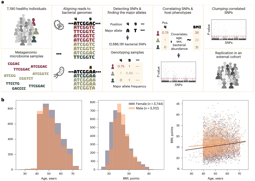
We devised a framework for MWASs to systematically detect nucleotide-level intra-species variability in the microbiome and identify associations between individual bacterial SNPs and host phenotypes (Fig. 1a). We used samples from 7,190 healthy individuals from Israel that we collected in this study as part of our ongoing ‘10K Project’21. Our cohort is, thus, one of the largest single cohorts of shotgun metagenomic microbiome samples that are coupled with host phenotypes.
Fig. 1 ∣. Study overview.
a, illustration of the study design. b, Age, sex and BMI distribution of the study participants. The purple and orange lines in the right panel show the trend of the age–BMI relation for females and males, respectively. The P value of the slope is 10−17 for the purple and 10−10 for the orange lines.
To detect SNPs, we compared metagenomic samples from different individuals. Using metagenomic samples rather than cultured isolates enabled the analysis of a large number of samples, which is essential for this study, and a wide taxonomic range. However, it relies on the alignment of short reads to reference genomes, which makes discriminating intra-species SNPs from inter-species variations more challenging. To restrict our analyses to variations within bacterial species, we took several measures to ensure that we assigned reads to the correct species. First, we aligned the sequenced reads to an expanded high-quality reference set of species that was recently assembled by our group22. This genome set, which was built using thousands of gut microbiome samples from Israeli individuals, best represents the variety of bacterial species expected to exist in our cohort. As a first step, we used the Unique Relative Abundances (URA) algorithm23, which uses genomic sequences that are unique to single species in the reference set to determine which bacterial species exist in each microbiome sample. Finally, we mapped the sequenced reads of each sample and excluded reads that could be assigned with the same likelihood to multiple species that existed in the sample (Methods).
After the read assignment step, we compared all reads assigned to the same genomic position to find the global major allele (that is, the most prevalent nucleotide in this position across the cohort) and computed the frequency of this allele within each sample covering this position—the ‘major allele frequency’. Finally, we filtered all genomic positions by their coverage (1,000 samples or more) and variability (average major allele frequency ≤ 99%; Methods). We found 12,686,191 positions that met these criteria, which we marked as SNPs, spread across the genomes of 348 of the bacterial species (Extended Data Fig. 1). The median number of SNPs detected in a genome was 3,221 SNPs, but 56 (16%) of the genomes had over 100,000 such variable positions.
We designed our MWAS framework to separately test each SNP’s association with host BMI, or any other trait of interest, following the common practice of human GWASs, which aims to discover associations between SNPs in the human genome and various phenotypes. In contrast to human genetics in which a person can have one, two or no copies of an allele, the bacterial population in the microbiome can have any number of allele copies. Therefore, we modeled each sample’s genotype as a continuous number in the range of 0 to 1, representing the ‘major allele frequency’—the frequency of the cohorts’ major allele out of the sample’s reads that mapped to a specific genomic position. For each SNP, we created a linear regression model with the major allele frequency as the independent variable and the BMI as the explained variable. With these models, we computed the statistical significance of the association between each SNP–trait pair, using the P value of the SNP estimated in the model. To isolate the SNP’s association with the phenotype in question from potentially confounding phenotypes (Fig. 1b), we used a common GWAS approach and added covariates for other host traits (age and sex; Methods). As an additional precaution to avoid mixing within-species and between-species variations, we also included the relative abundance of the species as a covariate. To account for the large number of hypotheses tested, we corrected all P values using the Bonferroni method. We only included participants with complete records for age, sex and BMI, resulting in the inclusion of 7,056 of the 7,190 participants.
Because the bacterial species colonizing the gut often diversify into multiple strains24, we assumed that some SNPs may be correlated due to population structure or linkage disequilibrium (LD)25-27. Our goal in this work was to find point variations that are independently associated with host BMI, and we wanted to avoid inflated results of correlated SNPs. To exclude redundant associations, we applied a clumping procedure that is common in GWASs as a final step in our MWAS analysis. In this clumping procedure, the SNPs associated with the phenotype are sorted by the P value of the association. The SNP with the smallest P value is selected first, and all SNPs that are correlated to it are removed from the results. Then, the SNP with the smallest P value of those left is analyzed, and this process continues until all SNPs are selected. This procedure results in a filtered list of SNPs that are each correlated with the phenotype and uncorrelated with each other. We applied this procedure to the results of each species separately, choosing a stringent correlation coefficient threshold of 0.3 (Methods).
Bacterial SNPs associate with host BMI
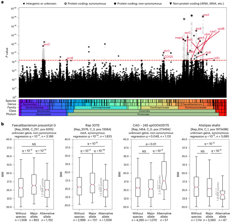
To investigate whether individual microbiome SNPs associate with host health, we applied our MWAS framework to test the association of each of the 12,686,191 bacterial SNPs with host BMI. We discovered 1,358 bacterial SNPs that are associated with host BMI (Bonferroni-corrected P < 0.05; Fig. 2, Extended Data Figs. 2 and 3 and Methods).
Fig. 2 ∣. Bacterial SNPs associate with host BMI.
a, Manhattan plot showing the P value of each SNP’s association with BMI. SNPs are sorted along the x axis based on taxonomy. The red dashed line marks the Bonferroni-adjusted 0.05 P value threshold = 3.94 × 10⁻⁹. SNPs that were excluded in the clumping stage are colored in light gray. Red annotations show gene symbols of the protein-coding SNPs left after the clumping stage (if a gene symbol exists). b, For the SNPs with the smallest P value (left two) or largest difference between allele groups (right two) out of the SNPs that were not filtered in the clumping stage, box plots (center, median; box, interquartile range; whiskers, 5th and 95th percentiles; notches, 95% confidence interval around the median based on 1,000 times bootstrap) compare host BMI distribution of individuals with no bacteria of this species (Methods), hosts of bacteria with the major allele (major allele frequency ≥ 0.99) and hosts of bacteria with the minor allele (major allele frequency ≤ 0.01). The gray line indicates the difference between medians. Groups were compared in a two-sided Mann–Whitney test, and P values were Bonferroni corrected for 120 hypotheses (40 SNPs, three comparisons per SNP). All 40 SNPs are shown in Extended Data Fig. 3. The q values in the titles are the Bonferroni-adjusted P values of SNPs in the original MWAS regression. NS, not significant.
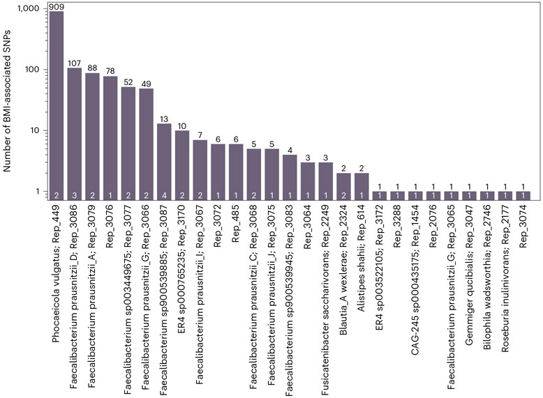
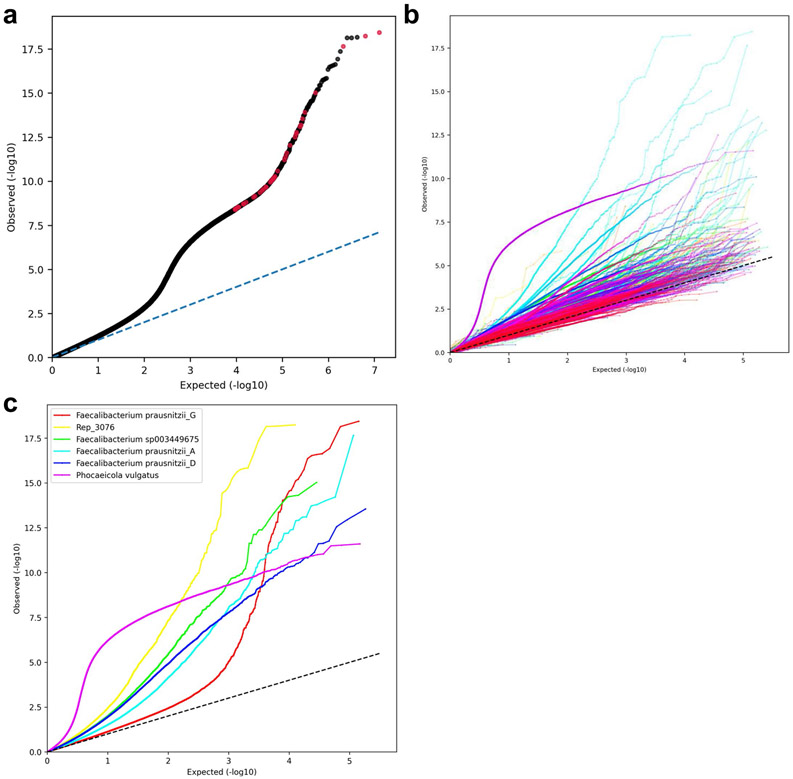
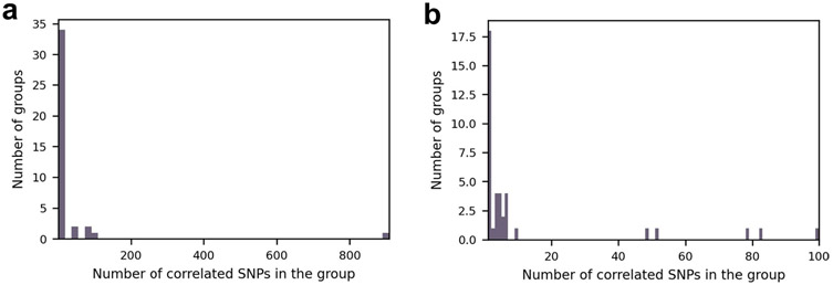
In most species in which we found BMI-associated SNPs, there were only 1–13 such SNPs (21/27; Fig. 3 and Supplementary Table 1). However, other species had 49–909 BMI-associated SNPs, which suggests that, in some species, there is a strain structure associated with BMI. This is further supported by the Q–Q plot (Extended Data Fig. 4). We then clumped these results to remove correlated SNPs. The clumping procedure reduced the number of uncorrelated BMI-associated SNPs in all species to four SNPs at most (Fig. 3, in white), implying that, in some species, there were indeed redundant associations arising due to LD and population structure (Extended Data Fig. 5). In total, after the clumping procedure, we ended up with 40 uncorrelated SNPs associated with BMI (Supplementary Tables 2 and 3).
Fig. 3 ∣. Number of BMI-associated SNPs per species.
Bar height and black numbers show the number of SNPs achieving the Bonferroni-adjusted 0.05 significance cutoff for association with BMI. White numbers show the number of associations retained after the clumping procedure. Species with no BMI-associated SNPs are not shown.
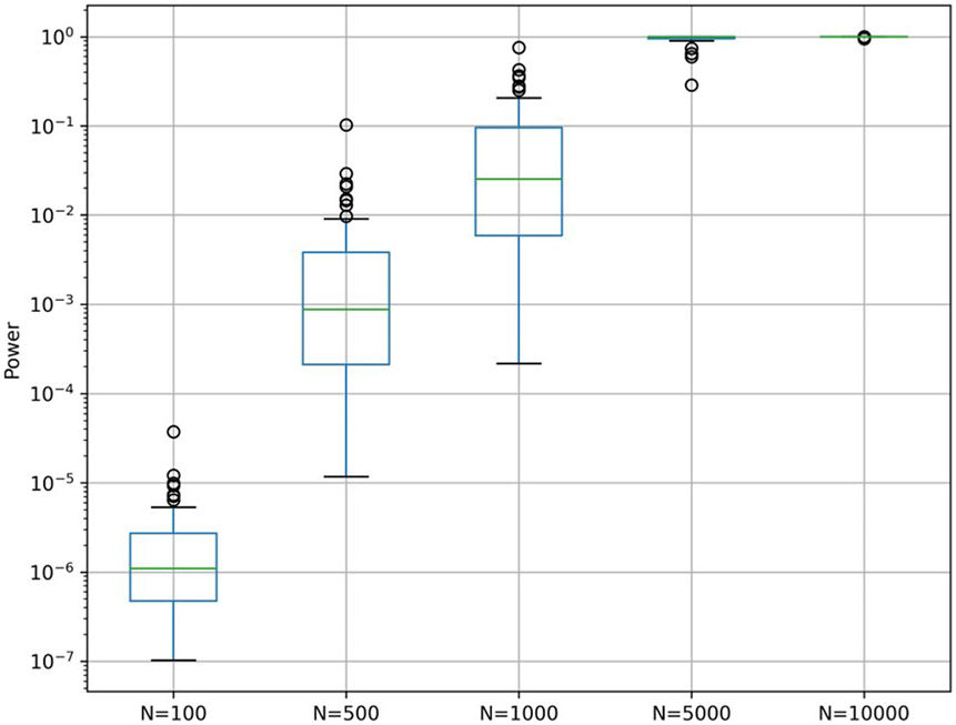
For the design of future MWAS studies, we used the estimated effect sizes of these 40 associations and calculated the statistical power of a similar MWAS analysis with various sample sizes (Methods). We found that using only 1,000 samples covering each SNP and without a prior hypothesis on specific SNPs, only one of the 40 associations had a 0.5 probability of being detected (Extended Data Fig. 6).
MWAS reveals associations independent of species-level analysis
A common approach to studying the human gut microbiome is associating species presence or relative abundance with host phenotypes. We were interested in the added value of the MWAS framework when investigating the relation between microbiome and health. For that aim, we compared the MWAS results with the species associated with host BMI by relative abundance. We found BMI-associated SNPs in the genomes of 27 different bacterial species. For each SNP–BMI association that we discovered, we investigated whether BMI is also associated with the relative abundance of the bacteria (Methods). In 44% (12/27; Fig. 4a and Supplementary Table 4) of cases in which a species has an SNP associated with BMI, the relative abundance of the species itself was not associated with the phenotype. Complementarily, 52% (21/40; Fig. 4b) of the BMI-associated SNPs that we discovered were in species that are not associated with BMI by their relative abundance. Thus, our SNP-level analysis identifies associations that exist at a higher level of resolution and often not in species relative abundance.
Fig. 4 ∣. Comparison of MWAS results and relative abundance analysis.
a, Pie plot shows the fraction of bacterial species not correlated with BMI by species relative abundance out of the 27 species in which we found BMI-associated SNPs. b, Pie plot shows which of the 40 BMI-associated SNPs are in species associated with BMI by relative abundance.
SNP–BMI associations replicate in an independent cohort
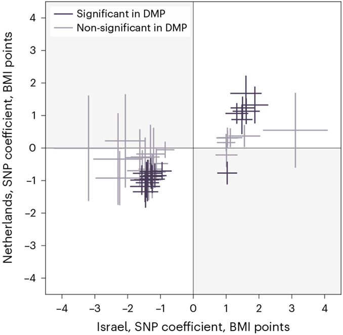
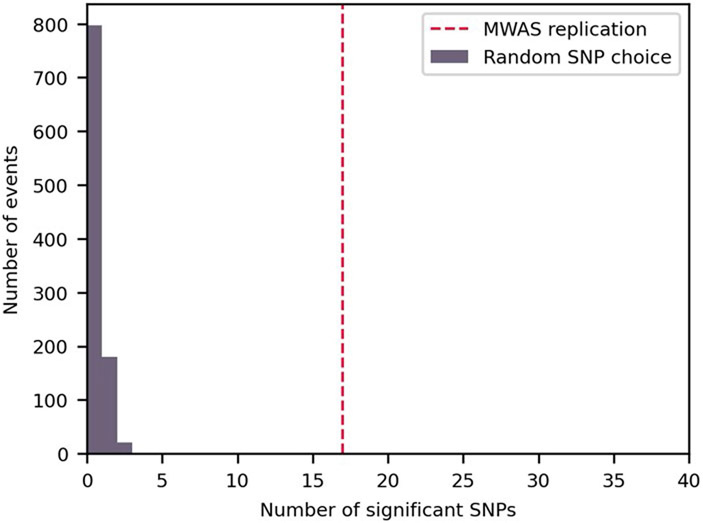
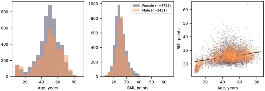
To assess the robustness and generalization of the above associations, we tested their replicability in samples from 8,204 individuals from the Netherlands (from the Dutch Microbiome Project cohort28). We tested all 40 SNPs, without filtering them for sample size or variability, which was, in some cases, lower in the second cohort. Notably, 17 of the 40 associations replicated (42.5%, Bonferroni-corrected P < 0.05; Fig. 5 and Supplementary Table 5) in this geographically and technically independent cohort. One additional SNP was significantly associated with BMI but in the opposite direction than in the Israeli cohort. We estimated the required sample size to replicate the associations (Methods) and found that, in five of the 23 associations that did not replicate in the second cohort, the sample size was too small to achieve the desired statistical power. To test the statistical significance of these results, we also tested 40 SNPs chosen at random and repeated this experiment 1,000 times. In no random set of 40 SNPs, we found in the Dutch cohort as many associations with BMI (P < 0.001, mean: 0.23, maximum: 4, s.d.: 0.48; Extended Data Fig. 7), implying that, even though the cohorts have different age, sex and BMI distributions (Fig. 1b and Extended Data Fig. 8), as well as different genetic and environmental backgrounds, the associations that we discovered are not random and replicate significantly. Additionally, we tested whether SNPs reveal associations beyond those of species relative abundance. We found that, of the 14 species in which we replicated SNP–BMI associations in the second cohort, seven species (accounting for eight of the 17 replicated associations; Supplementary Table 6) did not have species-level relative abundance associations with BMI, demonstrating, again, the additional information found at the SNP level.
Fig. 5 ∣. Results replicate in a geographically independent cohort.
Comparison of each SNP’s estimated coefficient (center) and 95% confidence interval (bars) in the MWAS regression in the discovery (x axis) and the replication (y axis) cohorts. SNPs are colored according to whether their Bonferroni-adjusted P value in the replication cohort is below 0.05. SNPs in the upper-right and lower-left quarters have the same correlation directionality in both cohorts.
SNP–BMI associations highlight specific loci
To investigate the mechanisms underlying the SNP–BMI associations and to account for additional confounders, we conducted additional MWAS analyses for the 40 SNPs. We added diet, medications and exercise covariates to the regression analysis and tested whether the SNP P value in the model still passes the significance threshold. Because we had only some features for every participant, we tested each feature group separately (Methods and Supplementary Table 8). When we added the diet data, one SNP stopped being significant. With the exercise features, we could test only 35 of the SNPs, of which one SNP stopped being significant. None of the SNPs stopped being significant with the addition of the medication data (Supplementary Tables 9-11). We concluded that diet and exercise may have confounded two of the SNP–BMI associations, possibly affecting both bacterial genetics and host obesity status independently. Most SNP–BMI associations could not be explained by diet, exercise or medications.
We next sought to characterize the functional context of BMI-associated SNPs. We reasoned that genomic regions in which variation is associated with host health traits might contain functions that are central to the interactions between the bacteria and the physiology of the host. We annotated the reference genomes and compared SNP positions with predicted gene locations (Methods and Supplementary Tables 2 and 3).
Half (20/40) of the BMI-associated SNPs that we found are in six species annotated as Faecalibacterium prausnitzii and three species annotated as other Faecalibacterium species. F.prausnitzii is known to associate with various host health conditions. Its abundance is negatively correlated with host obesity29, and, in a Mendelian randomization analysis, it was shown to have a causal role in reduced trunk fat mass30.
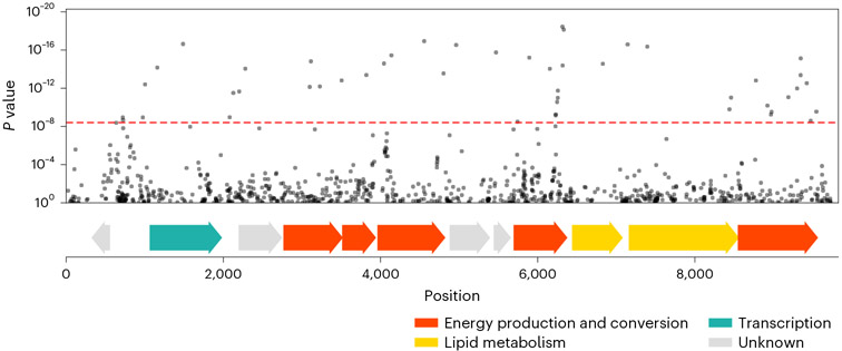
The SNP whose association with BMI was the most statistically significant is a non-synonymous polymorphism in a Faecalibacterium prausnitzii_G (Rep_3066) genome, within a predicted gene suspectedly encoding a flavodoxin—a redox-active protein. In the clumping analysis, we found that this SNP correlates with 47 other BMI-associated SNPs (Supplementary Table 7), all located within an 8,825-bp region. We conducted a functional enrichment analysis and discovered that the BMI-associated SNPs in this region are enriched with genes predicted to code for energy production and conversion function (P < 1 × 10⁻³⁰; Methods and Fig. 6). It was suggested that a way in which different gut microbiome compositions affect the risk of obesity is through variation in the efficiency of extracting energy from food31. A possible explanation for the associations between these SNPs, which reside in metabolic genes, and host BMI is that the SNPs affect the metabolic efficiency of the bacteria and consequently affect host BMI.
Fig. 6 ∣. BMI-associated SNPs in Rep_3066.
Top plot, a fraction of the Manhattan plot from Fig. 2a, zoomed-in to show a region of Rep_3066, contig 257, where there are SNPs significantly associated with BMI. SNPs are plotted according to their genomic position (x axis) and P value (y axis). The red dashed line marks the Bonferroni-adjusted 0.05 P value threshold. In the clumping procedure, the SNP with the smallest P value was retained, and other significantly associated SNPs were filtered out. Bottom plot, position of predicted ORFs in the shown genomic region, colored based on their predicted function.
When there are multiple SNPs within a genome that are all correlated with the trait as well as with each other, we cannot directly deduce which genetic variation has led to the functional difference that underlies the association with the host. Some of the correlated SNPs may have no effect on the bacteria–BMI interaction and correlate with BMI only because the SNPs are correlated—due to ancestry or LD—with variations that affect this interaction. Of the 40 SNPs that passed the clumping process, 18 represent singleton associations that were not correlated with any other BMI-associated SNP in the genome (that is, independent associations; Extended Data Fig. 2). We assumed that these SNPs are more likely to point toward the functional differences that directly affect host–bacteria interactions.
One of these singleton SNPs is in the genome of Bilophila wadsworthia (Rep_2746). It is thought that part of the influence of diet on obesity and obesity-related metabolic disorders is mediated by the activation of the immune system and a persistent state of low-grade inflammation32. There is evidence showing that this effect is mediated by microbiome lipopolysaccharide (LPS), a component of the outer membrane of Gram-negative bacteria and a potent activator of the immune system. For example, a study in mice showed that, after a high-fat diet (HFD), serum LPS levels increased and that continuously injecting mice with LPS promoted weight gain and insulin resistance33. Specifically, B. wadsworthia was shown to expand in the microbiomes of mice on an HFD, and, when mice on an HFD were colonized with this species, microbiome LPS gene expression and host inflammation markers increased34. Interestingly, the BMI-associated SNP that we discovered in B. wadsworthia genome was located in a gene coding for UDP-4-amino-4-deoxy-l-arabinose-oxoglutarate aminotransferase, an enzyme modifying an arabinose that is attached to lipid A. Lipid A is the most immunogenic component of LPS; its different modifications have great effect on the nature of the immune response and are adaptive to different environments35. Notably, this SNP was the one whose association with BMI lost its statistical significance with the addition of the diet covariates to the regression model. Taken together, we suggest that the genetic variation that we discovered interacts with the host diet and affects the levels or toxicity of LPS expressed by the bacteria and, consequently, may cause the host to gain weight.
Discussion
Although various bacterial species in the gut microbiome are known to associate with host health, the association of single-nucleotide variations with human health traits was not yet tested. In this work, we associated 12,686,191 bacterial SNPs with host BMI in a cohort of 7,190 healthy individuals. We discovered 1,358 associations between individual bacterial SNPs and host BMI, which represent 40 independent associations—considerably unconfounded by host diet, medications and physical activity and tested in an independent cohort. Although this study concentrated on BMI, both we and others can harness this versatile metagenomics-based framework for studying other traits, cohorts and body sites, to further the understanding of the associations between the microbiome and host health. We demonstrate that nucleotide-level intra-species diversity in the microbiome correlates with the diversity in human physiological states, highlighting the potential importance of incorporating this level of information, previously unaccounted for, in future studies of host–microbiome interactions.
We show the advantage of the MWAS framework in creating mechanistic hypotheses. Each of the associations that we found can be mapped to a specific bacterium, gene and even protein domain and can be further studied in its functional context. By contrast, SNP arrays used in most human GWASs provide only limited subsets of SNPs and may not identify causal SNPs. In this analogy, the MWAS framework is more similar to whole genome sequencing-based GWASs, which directly test all variable nucleotides and can point directly at causal loci. Our study highlights two associations related to energy metabolism and host inflammatory state that support leading hypotheses on the microbiome’s impact on host weight while also identifying genes with unknown function that call for further study and annotation.
We revealed 40 associations between bacterial SNPs and host BMI that may potentially improve future microbiome-based interventions. Some of the BMI-associated SNPs that we discovered may have a causal role. Alternatively, some of the phenotype-associated SNPs that we discovered may be adaptive. Zhao et al.36 showed that gut bacteria evolve at the nucleotide level during a host’s lifetime, but they did not compare these changes with physiological or exogenous host factors. The SNPs that we found may reflect the effect of host health and lifestyle on the microbiome. The two options are not necessarily mutually exclusive. Boehme et al.37 showed that fecal microbiota transplantation from young to old mice reverses some of the immune and cognitive effects of aging. This implies that, although the aging process affects the gut microbiome, the microbiome, in turn, has a causal role in some of the phenotypic differences associated with aging. Similarly, the abundance of various genetic variants may result from host lifestyle, for example, as well as affect host health. Identifying the causal nature of these associations necessitates a subsequent SNP-based microbiota transplantation study. This intricate task would require the isolation and cultivation of the specific strains, genetic manipulation to introduce individual variation and the development of an appropriate model system for a comprehensive exploration of the SNP impacts on both the bacteria and host. Such follow-up experimental work will also enable the validation of the independence of SNP associations with BMI from associations with bacterial relative abundance, which was, thus far, supported for all associations by using relative abundance as a covariate in the MWAS model and for a subset of associations by the lack of direct correlation between relative abundance and BMI.
Associations that result from causal SNPs, once validated, may be utilized for the development of therapeutics. Since the associations we found map to a specific genomic position, such treatments may be based on administering the bacteria with the health-associated alleles, the enzyme which contains the health-associated residue, or the metabolic product of the enzyme variants. Some of the SNPs we found show a large phenotypic difference between individuals with the major or alternative alleles. For some SNPs, the average BMI difference between the allele groups was greater than 2 points—the equivalent of a 5.8 kg difference for a 1.7 meters tall person. If causal, treatments based on the SNPs can potentially have large effect sizes. Adaptive SNPs can also be used to improve microbiome-based treatments. In addition to their contribution to our general understanding of host-microbiome interactions, variants that are adapted to certain health states may be the basis for more robust—and possibly, personalized—microbiome modifications.
We note that this is not an exhaustive set. BMI-associated SNPs may be absent from our results because we filtered out reads from genomic regions shared between species or for bacteria that were not prevalent enough to reach the 1,000 samples cutoff for inclusion or for the association to reach the metagenome-wide significance cutoff. Our results show the potential of the MWAS framework to shed light on the mechanisms underlying host–microbiome interactions, but the comprehensive interpretation of the MWAS results is still limited by our understanding of microbiome population structure. Although methods to control for population structure were developed in the field of human genetics, their translation into the metagenomic microbiome world is not straightforward: metagenotyping hinders the deduction of long-range linkage and haplotyping38, especially for low-abundance species and when using single-end sequencing; principal component analysis (PCA), which is often used in GWASs to account for population structure, is also problematic in a metagenomic framework due to the high missingness in the data. Basing the study on cultured isolates rather on metagenomic sequencing could have helped resolve the population structure but at the expense of sample size and taxonomic range. We aimed for a systematic analysis of microbiome SNPs across species and, therefore, prioritized obtaining a large sample size by using metagenomic data and including both low-coverage and high-coverage species and samples. The existence of population structure and linked SNPs can lead to false discoveries due to correlation among SNPs, population stratification, structural variations or pangenome variations. It may also lead to missed discoveries because testing many correlated SNPs independently and multiple-hypotheses adjustments impairs the statistical power in the study. In one species, we originally found 908 correlated BMI-associated SNPs. In this species, the large number of correlated SNPs may indicate that there are separate strains that are associated with host BMI, perhaps through nucleotide variation but possibly due to other strain differences, such as gene content variations, which were not the focus of this study.
Because, in most species, we found fewer than a dozen BMI-associated SNPs, we assume that, in these species, the associations that we discovered were probably not confounded by population structure. Additionally, we adopted the GWAS clumping procedure to remove redundant associations and identify singleton SNPs whose associations with the phenotype are more likely direct. This further increased the MWAS potential to highlight specific loci of potential importance to host–microbiome interactions and separate those from correlated SNPs that result from population structure and LD. The clumping procedure revealed that some SNPs were correlated, which implies that we lost statistical power—the number of independent hypotheses that we tested in the study is smaller than the number that we corrected for. Although we likely set the Bonferroni thresholds too high for that reason, we nonetheless discovered numerous significant associations. Finally, although additional validation is needed, observing the correlation between SNPs and BMI in a second cohort of people from a different continent, which represent different host and bacterial ancestry, also reduces the likelihood of population stratification and other population structure biases. Future research can further improve the MWAS framework by developing more MWAS-appropriate methods to account for bacterial population structure.
In summary, we presented a framework to study the associations between single-nucleotide variations in the microbiome and host phenotypes and show that individual SNPs in the microbiome associate with host BMI. These associations can be mapped to specific loci, suggesting specific genes that may stand at the center of host–microbiome associations for future studies and may pave the way to designing novel microbiome-based treatments.
Methods
Cohort
We analyzed a cohort of 7,190 healthy Israeli individuals. Participants in this cohort included 3,816 (53.1%) women and 3,374 men who were recruited as part of an ongoing prospective study—’the 10K Project’21. Ages ranged from 25 years to 75 years, and most were between 40 years and 70 years (7,116/7,190, 99%). Exclusion criteria are detailed in Shilo et al.21 and include antibiotics usage in the 3 months before recruitment. A single sample from each participant was included in this observational study. Samples were collected between April 2019 and March 2022.
The year of birth and the sex of the participants were self-reported. BMI was calculated based on height and weight that were measured on site. We handled outliers in the BMI measurements using the following procedure: first, we found the fraction of the data that includes 98% of the values within the smallest range; next, we calculated the mean and s.d. of BMI distribution, based on these 98% of the data; and then, we removed values that are more than 9 s.d. away from the mean and clipped values that are 5 s.d. away from the mean or farther. We obtained complete age, sex and BMI data for 7,056 of the 7,190 participants and removed the remaining individuals from the analysis. Diet, medication and exercise habits data were also self-reported. Diet was self-recorded using a designated mobile app in the 14-d period around sampling.
All participants signed an informed consent form upon arrival to the research site. The 10K cohort study is conducted according to the principles of the Declaration of Helsinki and was approved by the institutional review board of the Weizmann Institute of Science (protocol no. 964-1).
Microbiome sample collection and processing
Microbiome sampling was done using an OMNIgene·GUT (OMR-200, DNA Genotek) stool collection kit, which has the advantage of maintaining DNA integrity in typical ambient temperature fluctuations. Each participant was given a kit and was requested to collect a fecal sample at home. The collected samples were transferred at room temperature to our participant reception center at Weizmann Institute of Science, where they were documented and frozen at −20 °C immediately. Then, samples were transferred in a cooler to our research facilities where they were stored at −20 °C until DNA extraction was performed. Laboratory work was done in the Segal laboratory at the Weizmann Institute of Science.
Metagenomic DNA was purified using PowerMag Microbial DNA Isolation Kit (MO BIO Laboratories, 27200-4) optimized for the Tecan automated platform. Libraries for next-generation sequencing were prepared using NEBNext Ultra II DNA Library Prep Kit for Illumina (New England Biolabs, E7775) and sequenced on a NovaSeq sequencing platform (Illumina). Sequencing was performed with a 100-bp single-end reads kit and a depth of 10 million reads per sample, using Illumina unique dual sequencing indexes (IDT–Syntezza Bioscience). DNA purification, library preparation and sequencing were performed in batches of 384 samples. A standard microbial community (ZymoBIOMICS Gut Microbiome Standard, D6331) was inserted into each batch for quality control. No batch corrections were performed.
We filtered metagenomic reads containing Illumina adapters and low-quality reads and trimmed low-quality read edges. We detected host DNA by mapping reads to the human genome using Bowtie 2 (ref. 39) with inclusive parameters and removed those reads.
Metagenomic reads mapping
We mapped the processed reads to a reference set of genomes representing bacterial species from the human gut microbiome. The reference set that we used, as well as the procedures for its taxonomic annotation, gene prediction and gene annotation, are described in detail in Leviatan et al.22.
We mapped the metagenomic reads to the reference genomes twice: first to estimate the list of bacterial species present in each sample and their relative abundances and then to compare reads aligned to the same genomic position at the SNP stage.
To determine species relative abundance in samples, we used the URA algorithm23, which uses genomic sequences that are unique to single species in the reference set to determine which bacterial species exist in each microbiome sample. We clipped the relative abundance at a minimum of 0.0001 (that is, this is the smallest possible value of a species relative abundance in this framework).
For the SNPs stage, we assigned each metagenomic read to a position within a bacterial genome using Bowtie2 (version 2.2.9, option ‘–very-sensitive-local’)39. If Bowtie2 found multiple target genomes to which the read could map with the same score, we compared the list of potential targets with the list of species that we assumed (based on the previous step) exist in the sample. When a read could be assigned with the same likelihood to more than one species that existed in the sample, we excluded it from the analysis. We chose this approach for two reasons: on the one hand, excluding ambiguously mapped reads is important for not mistaking polymorphisms that mark the difference between different species with a similar genomic region as actual (intra-species) SNPs; on the other hand, considering only species present in each sample as potential targets helped us retain more reads and increase the sample size.
Finding variable positions, calling the major allele and genotyping samples
The first step was to find the cohort-wide major of each genomic position of each species in our samples. For each position within the reference genome, for each sample, we counted the number of reads that mapped to this position containing each of the four nucleotides (up to a limit of 255 reads per nucleotide per sample). Then, for each position, we summed these four values over all of the samples that covered this genomic position to determine the cohort-wide major allele of that position as well as the second major allele. We note that this stage also included samples that are not included in this study (from other cohorts that we analyze in our group23,40), which may have affected our perception of the cohort-wide major allele.
Next, we genotyped the samples. For each sample and each genomic position, we computed the fraction of reads that contained the cohort-wide major allele—its major allele frequency.
Lastly, we detected the variable positions. We binarized each sample as either ‘major’ or ‘non-major’ (major allele frequency > 0.05 or major allele frequency ≤ 0.05, respectively) and marked as ‘SNPs’ the positions in which the fraction of samples with mostly the major allele was at most 99% of the samples covering the positions, based on the common definition for SNP.
Statistics and reproducibility
No sample size calculations were done as part of the study design. Because this is the first study, to our knowledge, to associate microbiome SNPs with host BMI, no prior knowledge on the expected effect sizes exists, and, thus, a sample size calculation was not feasible. Samples included are all the samples that met the criteria described in the ‘Cohort’ subsection.
Data analysis was done using Python 3.7.4, with packages numpy 1.21.0, pandas 1.2.5, statsmodels 0.12.2 and scipy 1.7.0.
SNP–phenotype associations
For each SNP that we associated with BMI, we excluded samples with any missing value for one of the covariates or for the explained variable. We then verified that (1) there remained at least 1,000 samples; (2) the position is sufficiently variable—there are at least 1% and at least 50 samples in which the dominant allele is the major allele and, similarly, at least 1% and 50 samples in which the dominant allele is different than the major allele; and (3) the most common value of the explained variable (that is, the most common BMI label among samples) is not more common than 95% of samples. We only analyzed SNPs that fulfilled all these criteria.
We tested the association between each SNP and BMI using a linear regression model with the microbial genotype (major allele frequency), species relative abundance (log10) of the species to which the SNP belongs, age and sex as covariates and the BMI value as the explained variable. Only samples with complete data were included in the analysis of each SNP.
For the linear regression, we used statsmodels.regression.linear_model.OLS41. We performed Bonferroni’s adjustment for the statistical significance 0.05 cutoff: 0.05 / 12,686,191 = 3.94 × 10⁻⁹.
Clumping
We applied the clumping procedure to extract independent associations from the list of BMI-associated SNPs. For each species separately, we began the process with the list of SNPs whose associations with BMI passed the significance threshold (metagenome-wide Bonferroni ≤ 0.05) and filtered it in an iterative procedure. In each step, we added to the final list the SNP with the smallest P value and removed from the analysis all SNPs that were correlated to it. In the next step, we added to the final list the SNP with the next-smallest P value (out of the SNPs that were not excluded in the previous step). This process removes from the list of BMI-associated SNPs those that are correlated with each other and keeps only one representative SNP from each correlated SNP group, based on its strongest association with BMI. To avoid including redundant associations in our final list of results, we chose a stringent threshold for correlation and excluded SNPs correlated with Spearman’s correlation coefficient equal to or higher than 0.3 (with P ≤ 0.05).
Power estimation
To estimate the power to discover the 40 BMI-associated SNPs using different sample sizes, we used statsmodels.stats.power.tt_solve_power41. We calculated the standardized effect size of each SNP based on the regression model in the discovery MWAS, dividing the SNP’s estimated coefficient by the s.d. of the coefficient and the squared root of the discovery sample size: standardized effect size = coef / (s.d.(coef) × sqrt (N)). We set the alpha to 3.9 × 10⁻⁹ based on a cutoff of 0.05 and a Bonferroni correction for 12,686,191 hypotheses. We repeated this calculation for varying sample sizes and set the power variable to ‘None’ for the algorithm to estimate it. It is important to note that ‘sample size’ in this case refers to the number of samples with reads covering the specific SNP, which is usually smaller than the total number of samples in a study and even smaller than the number of samples including the species.
We estimated the sample required sample size for the replication in a similar manner, setting the sample size to ‘None’, the power to 0.9 and the alpha to 0.05 / 40 based on a cutoff of 0.05 and a Bonferroni correction for 40 hypotheses.
Associating phenotypes with species abundance
For each species in which we found SNPs significantly associated with BMI, we tested whether the relative abundance of the species also associates with this phenotype. We excluded samples for which the BMI value was missing and computed the P value of the Spearman’s correlation between the relative abundance of species and BMI (using scipy.stats.spearmanr42). We performed Bonferroni’s adjustment for multiple hypotheses by multiplying each P value by the total number of species tested and setting the significance threshold at 0.05.
Replication in a second cohort
We obtained the metagenomic samples from Gacesa et al.28 and processed them using the same computational pipeline that we used for the discovery cohort. To use the same pipeline, we used only one of the paired-end reads (either forward or reverse) and truncated reads at 75 bp. We repeated the MWAS analysis for the 40 SNPs that were significantly associated with BMI in the discovery cohort. We tested all 40 SNPs, even if they did not meet the criteria set for SNPs in the discovery MWAS; we did not require a minimum sample size, variability in the SNP among tested samples or variability in the BMI. We performed Bonferroni’s adjustment for the statistical significance 0.05 cutoff: 0.05 / 40 = 0.00125.
Replication randomization
To estimate the statistical significance of the replication rate of the associations in the second cohort, we tested how many significant associations could be found in a random set of 40 SNPs. We repeated this experiment 1,000 times, each time choosing 40 of the SNPs that were tested in the discovery MWAS for an MWAS analysis with the replication cohort. We used the same parameters as described in the ‘Replication in a second cohort’ subsection and corrected for 40 hypotheses in each repetition. In 137 of the 1,000 repetitions, one or two SNPs could not be analyzed. We then compared the number of statistically significant associations found in each random set of 40 SNPs with the number of associations found when testing the 40 SNPs that were associated with BMI in the discovery cohort. In none of the 1,000 repetitions did we find as many statistically significant associations, and, thus, we estimated the P value for the replication to be less than 0.001.
Controlling for additional confounders
To analyze the potentially confounding effect of host diet, exercise and medications on the SNP–BMI associations, we repeated the MWAS analysis of the 40 post-clumping BMI-associated SNPs with additional covariates. We only included medication categories reported by at least 50 participants. Diet covariates of each participant were generated by dividing the logged food items into categories, calculating the daily fraction of caloric intake attributed to each food category and averaging these fractions over days with at least 500 logged calories. Diet, exercise and medication covariates are listed in Supplementary Table 7.
Because our records for these self-reported features are partial, and because, for each SNP, we only analyzed samples with complete covariate information, the addition of each covariate reduced the sample size for the MWAS. Therefore, we tested each of the three categories separately. For each of the 40 SNPs, after reducing the set of samples to those with complete information on the additional covariates, we conducted a second regression analysis with the original set of covariates: the bacterial genotype and relative abundance, age and sex. Only if the SNP passed the statistical significance cutoff again, we conducted a third regression analysis, adding the extra covariates of the analyzed category. If the SNP–BMI association met the significance cutoff with the reduced set of samples but was not significant after adding the extra covariates, we deduced that the association might be confounded by the lifestyle variables of that category.
Annotating SNPs
To functionally annotate each SNP, we compared its genomic position with the location of predicted genes along the reference genome. Accordingly, SNPs were annotated as either within a gene or in an intergenic region. In some contigs, there were no predicted genes. In those, we marked the function of the SNPs as unknown. We further classified SNPs that were within predicted genes as either within protein-coding genes or within non-protein-coding genes (mainly RNA genes, such as tRNA and rRNA).
To determine the synonymy of SNPs within protein-coding genes, we compared its surrounding codon with the SNP’s major allele and with its second major allele. First, we compared the location of the SNP with the predicted open reading frame (ORF) to compute the location of the SNP’s surrounding codon. Then, we extracted the cohort-wide major allele of the three nucleotides within its surrounding codon. Finally, we compared the amino acid translation of this codon with the translation of the codon when the SNP’s allele is changed to its second major allele. If the two codons translated to different amino acids, we classified the SNP as non-synonymous.
Because we designed our MWAS framework to test the effect of each individual SNP independently, we did not test whether more than one SNP existed within a codon. In these cases, our synonymy classification may be wrong. Additionally, we note that, in samples where the allele is neither the cohort-wide major nor its second major, the effect of the genetic variation on the coded protein may be different than we predicted.
Functional enrichment
To test the potential functional enrichment of the 48 correlated BMI-associated SNPs in Rep_3066, we compared the fraction of SNPs in genes annotated with the COG category ‘C: Energy production and conversion’ out of all tested Rep_3066 SNPs, with the fraction of this COG category among the 48 SNPs. We used a hypergeometric distribution (scipy.stats.hypergeom42) to estimate the likelihood of obtaining these many ‘C’ category genes among the BMI-associated SNPs with a random choice of Rep_3066 SNPs.
Visualization
For visualization, we used Matplotlib43. To minimize the overlap between gene tags in Manhattan and volcano plots, we used adjust-Text (https://github.com/Phlya/adjustText; ref. 44).
Extended Data
Extended Data Fig. 1 ∣. SNPs overview.
(a) Distribution of the 12,686,191 detected SNPs across 348 species. (b) Number of samples covering different SNPs.
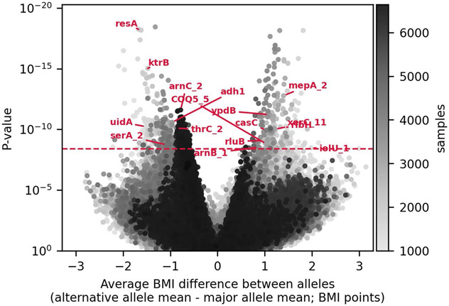
Extended Data Fig. 2 ∣. Volcano plot.
Volcano plot shows for each SNP the difference between the average BMI in individuals with mostly the alternative allele (major allele frequency ≤ 0.5) and the average BMI in individuals with mostly the major allele (major allele frequency > 0.5; x-axis); and its p-value (y-axis). Red annotations show gene symbols of the protein-coding SNPs left after the clumping stage (if a gene symbol exists). X-axis was truncated to the range of statistically significant associations ±10%.
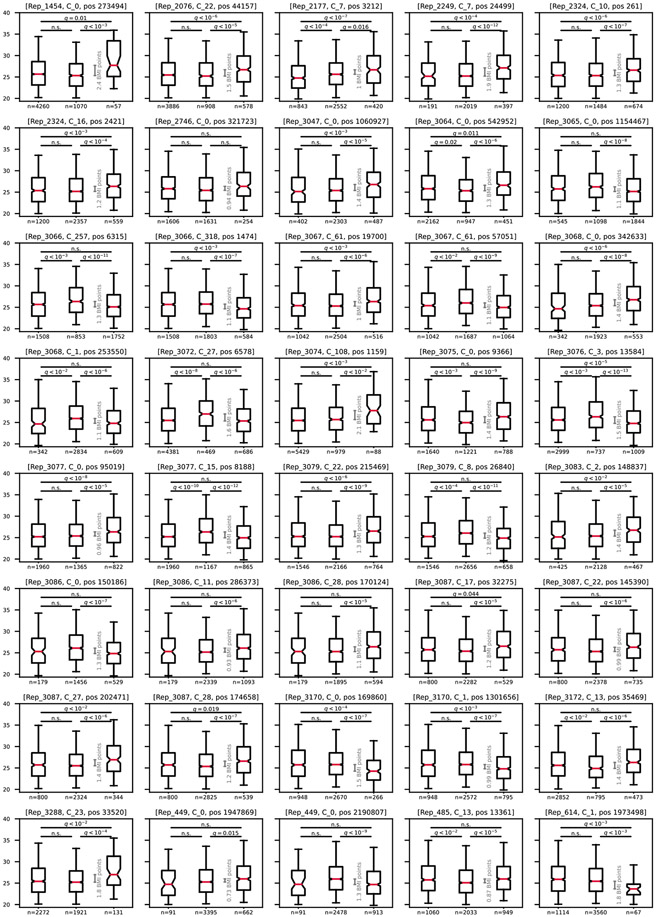
Extended Data Fig. 3 ∣. BMI differences.
For each of the 40 BMI-associated SNPs that remained after the clumping stage, boxplots (center, median; box, interquartile range; whiskers, 5th and 95th percentiles; notches, 95% confidence interval around the median based on 1,000 times bootstrap) compare host BMI distribution of individuals with no bacteria of this species (left box; Methods), hosts of bacteria with the major allele (middle box; major allele frequency ≥ 0.99) and hosts of bacteria with the minor allele (right box; major allele frequency ≤ 0.01). The grey scale indicates the difference between medians. Groups were compared in a two-sided Mann-Whitney test, and p-values were Bonferroni corrected for 120 hypotheses (40 SNPs, 3 comparisons per SNP).
Extended Data Fig. 4 ∣. Quantile-quantile (Q-Q) plots.
Expected (uniform distribution between 1/[the total number of tested SNPs] and 1) p-values compared to the SNPs p-values estimated in the MWAS analysis. (a) All tested SNPs. Red dots are the 40 BMI-associated SNPs remaining after the clumping procedure. (b) Each species estimated and plotted separately using a random color. Straight lines connect adjacent SNP dots to increase readability. (c) Species with more than 13 BMI-associated SNPs. Straight lines connect adjacent SNP dots to increase readability.
Extended Data Fig. 5 ∣. Number of correlated SNPs in each linkage group.
Histograms show the number of correlated SNPs that were found in the clumping stage in each linkage group. The total number of groups is 40, which is the final number of SNPs that remained post the clumping procedure. (a) Full range of group sizes. (b) Groups with 1 to 100 SNPs.
Extended Data Fig. 6 ∣. Power analysis.
Boxplots (center, median; box, interquartile range; whiskers, 1.5 * interquartile range or the most extreme data point) show the calculated power for associating the 40 SNPs with BMI, given the effect size observed in our cohort and various effective sample sizes (N). Alpha was set to 3.9 × 10⁻⁹ based on a cutoff of 0.05 and a Bonferroni correction for 12,686,191 hypotheses.
Extended Data Fig. 7 ∣. Random replication control.
For 1000 random choices of 40 SNPs from the discovery analysis, showing how many passed the 0.05 Bonferroni adjusted cutoff for association with BMI in the replication cohort. For reference, the red dotted line shows the number of SNPs that passed the cutoff when the 40 SNPs that were associated with BMI in the discovery cohort were tested – 17.
Extended Data Fig. 8 ∣. Replication cohort characteristics.
Age, sex, and BMI distribution of the 8,204 study participants.
Supplementary Material
Acknowledgements
We thank members of the Segal laboratory for useful discussions. E.S. is supported by the Crown Human Genome Center; the Larson Charitable Foundation New Scientist Fund; the Else Kröner Fresenius Foundation; the White Rose International Foundation; the Ben B. and Joyce E. Eisenberg Foundation; the Nissenbaum Family; Marcos Pinheiro de Andrade and Vanessa Buchheim; Lady Michelle Michels; Aliza Moussaieff; and grants funded by the Minerva Foundation, with funding from the Federal German Ministry for Education and Research and by the European Research Council and the Israel Science Foundation. S.S. is supported by the Israeli Council for Higher Education via the Weizmann Data Science Research Center. The funders had no role in study design, data collection and analysis, decision to publish or preparation of the manuscript.
Footnotes
Online content
Any methods, additional references, Nature Portfolio reporting summaries, source data, extended data, supplementary information, acknowledgements, peer review information; details of author contributions and competing interests; and statements of data and code availability are available at https://doi.org/10.1038/s41591-023-02599-8.
Reporting summary
Further information on research design is available in the Nature Portfolio Reporting Summary linked to this article.
Competing interests
O.W. is an employee of Eleven Tx. E.S. is a paid consultant for Pheno.AI. The other authors declare no competing interests.
Extended data is available for this paper at https://doi.org/10.1038/s41591-023-02599-8.
Supplementary information The online version contains supplementary material available at https://doi.org/10.1038/s41591-023-02599-8.
Data availability
Data in this paper are part of the Human Phenotype Project. The raw metagenomic data and basic phenotypes (age, sex and BMI) used in this study are available at the European Genome-phenome Archive (https://ega-archive.org/) under accession EGAS00001007204. The other data are accessible to researchers from universities and other research institutions at https://humanphenotypeproject.org/home.
Code availability
Analysis source code is available at https://github.com/LironZa/MWAS.
References
- 1.Lynch SV & Pedersen O The human intestinal microbiome in health and disease. N. Engl. J. Med 375, 2369–2379 (2016). [DOI] [PubMed] [Google Scholar]
- 2.Manichanh C. et al. Reduced diversity of faecal microbiota in Crohn’s disease revealed by a metagenomic approach. Gut 55, 205–211 (2006). [DOI] [PMC free article] [PubMed] [Google Scholar]
- 3.Tang WHW et al. Intestinal microbial metabolism of phosphatidylcholine and cardiovascular risk. N. Engl. J. Med 368, 1575–1584 (2013). [DOI] [PMC free article] [PubMed] [Google Scholar]
- 4.Turnbaugh PJ et al. A core gut microbiome in obese and lean twins. Nature 457, 480–484 (2009). [DOI] [PMC free article] [PubMed] [Google Scholar]
- 5.Karlsson FH et al. Gut metagenome in European women with normal, impaired and diabetic glucose control. Nature 498, 99–103 (2013). [DOI] [PubMed] [Google Scholar]
- 6.Yoshimoto S. et al. Obesity-induced gut microbial metabolite promotes liver cancer through senescence secretome. Nature 499, 97–101 (2013). [DOI] [PubMed] [Google Scholar]
- 7.Gopalakrishnan V, Helmink BA, Spencer CN, Reuben A & Wargo JA The influence of the gut microbiome on cancer, immunity, and cancer immunotherapy. Cancer Cell 33, 570–580 (2018). [DOI] [PMC free article] [PubMed] [Google Scholar]
- 8.Maruvada P, Leone V, Kaplan LM & Chang EB The human microbiome and obesity: moving beyond associations. Cell Host Microbe 22, 589–599 (2017). [DOI] [PubMed] [Google Scholar]
- 9.De Filippis F. et al. Distinct genetic and functional traits of human intestinal Prevotella copri strains are associated with different habitual diets. Cell Host Microbe 25, 444–453 (2019). [DOI] [PubMed] [Google Scholar]
- 10.Brito IL et al. Mobile genes in the human microbiome are structured from global to individual scales. Nature 535, 435–439 (2016). [DOI] [PMC free article] [PubMed] [Google Scholar]
- 11.Greenblum S, Carr R & Borenstein E Extensive strain-level copy-number variation across human gut microbiome species. Cell 160, 583–594 (2015). [DOI] [PMC free article] [PubMed] [Google Scholar]
- 12.Zeevi D. et al. Structural variation in the gut microbiome associates with host health. Nature 568, 43–48 (2019). [DOI] [PubMed] [Google Scholar]
- 13.Yoshida H, Bogaki M, Nakamura M & Nakamura S Quinolone resistance-determining region in the DNA gyrase gyrA gene of Escherichia coli. Antimicrob. Agents Chemother. 34, 1271–1272 (1990). [DOI] [PMC free article] [PubMed] [Google Scholar]
- 14.Viana D. et al. A single natural nucleotide mutation alters bacterial pathogen host tropism. Nat. Genet 47, 361–366 (2015). [DOI] [PMC free article] [PubMed] [Google Scholar]
- 15.Read TD & Massey RC Characterizing the genetic basis of bacterial phenotypes using genome-wide association studies: a new direction for bacteriology. Genome Med. 6, 109 (2014). [DOI] [PMC free article] [PubMed] [Google Scholar]
- 16.Schloissnig S. et al. Genomic variation landscape of the human gut microbiome. Nature 493, 45–50 (2013). [DOI] [PMC free article] [PubMed] [Google Scholar]
- 17.Shi ZJ et al. Fast and accurate metagenotyping of the human gut microbiome with GT-Pro. Nat. Biotechnol 40, 507–516 (2022). [DOI] [PubMed] [Google Scholar]
- 18.Olm MR et al. inStrain profiles population microdiversity from metagenomic data and sensitively detects shared microbial strains. Nat. Biotechnol 39, 727–736 (2021). [DOI] [PMC free article] [PubMed] [Google Scholar]
- 19.Maini Rekdal V, Bess EN, Bisanz JE, Turnbaugh PJ & Balskus EP Discovery and inhibition of an interspecies gut bacterial pathway for Levodopa metabolism. Science 364, eaau6323 (2019). [DOI] [PMC free article] [PubMed] [Google Scholar]
- 20.Wang J & Jia H Metagenome-wide association studies: fine-mining the microbiome. Nat. Rev. Microbiol 14, 508–522 (2016). [DOI] [PubMed] [Google Scholar]
- 21.Shilo S. et al. 10 K: a large-scale prospective longitudinal study in Israel. Eur. J. Epidemiol 36, 1187–1194 (2021). [DOI] [PubMed] [Google Scholar]
- 22.Leviatan S, Shoer S, Rothschild D, Gorodetski M & Segal E An expanded reference map of the human gut microbiome reveals hundreds of previously unknown species. Nat. Commun 13, 3863 (2022). [DOI] [PMC free article] [PubMed] [Google Scholar]
- 23.Rothschild D. et al. An atlas of robust microbiome associations with phenotypic traits based on large-scale cohorts from two continents. PLoS ONE 17, e0265756 (2022). [DOI] [PMC free article] [PubMed] [Google Scholar]
- 24.Truong DT, Tett A, Pasolli E, Huttenhower C & Segata N Microbial strain-level population structure and genetic diversity from metagenomes. Genome Res. 27, 626–638 (2017). [DOI] [PMC free article] [PubMed] [Google Scholar]
- 25.Power RA, Parkhill J & de Oliveira T Microbial genome-wide association studies: lessons from human GWAS. Nat. Rev. Genet 18, 41–50 (2017). [DOI] [PubMed] [Google Scholar]
- 26.Earle SG et al. Identifying lineage effects when controlling for population structure improves power in bacterial association studies. Nat. Microbiol 1, 16041 (2016). [DOI] [PMC free article] [PubMed] [Google Scholar]
- 27.Chen PE & Shapiro BJ The advent of genome-wide association studies for bacteria. Curr. Opin. Microbiol 25, 17–24 (2015). [DOI] [PubMed] [Google Scholar]
- 28.Gacesa R. et al. Environmental factors shaping the gut microbiome in a Dutch population. Nature 604, 732–739 (2022). [DOI] [PubMed] [Google Scholar]
- 29.Leylabadlo HE et al. The critical role of Faecalibacterium prausnitzii in human health: an overview. Microb. Pathog 149, 104344 (2020). [DOI] [PubMed] [Google Scholar]
- 30.Xu Q. et al. Mendelian randomization analysis reveals causal effects of the human gut microbiota on abdominal obesity. J. Nutr 151, 1401–1406 (2021). [DOI] [PubMed] [Google Scholar]
- 31.Turnbaugh PJ et al. An obesity-associated gut microbiome with increased capacity for energy harvest. Nature 444, 1027–1031 (2006). [DOI] [PubMed] [Google Scholar]
- 32.Das B, Das M, Kalita A & Baro MR The role of Wnt pathway in obesity induced inflammation and diabetes: a review. J. Diabetes Metab. Disord 20, 1871–1882 (2021). [DOI] [PMC free article] [PubMed] [Google Scholar]
- 33.Cani PD et al. Metabolic endotoxemia initiates obesity and insulin resistance. Diabetes 56, 1761–1772 (2007). [DOI] [PubMed] [Google Scholar]
- 34.Natividad JM et al. Bilophila wadsworthia aggravates high fat diet induced metabolic dysfunctions in mice. Nat. Commun 9, 2802 (2018). [DOI] [PMC free article] [PubMed] [Google Scholar]
- 35.Needham BD & Trent MS Fortifying the barrier: the impact of lipid A remodelling on bacterial pathogenesis. Nat. Rev. Microbiol 11, 467–481 (2013). [DOI] [PMC free article] [PubMed] [Google Scholar]
- 36.Zhao S. et al. Adaptive evolution within gut microbiomes of healthy people. Cell Host Microbe 25, 656–667 (2019). [DOI] [PMC free article] [PubMed] [Google Scholar]
- 37.Boehme M. et al. Microbiota from young mice counteracts selective age-associated behavioral deficits. Nat. Aging 1, 666–676 (2021). [DOI] [PubMed] [Google Scholar]
- 38.Garud NR & Pollard KS Population genetics in the human microbiome. Trends Genet. 36, 53–67 (2020). [DOI] [PubMed] [Google Scholar]
- 39.Langmead B & Salzberg SL Fast gapped-read alignment with Bowtie 2. Nat. Methods 9, 357–359 (2012). [DOI] [PMC free article] [PubMed] [Google Scholar]
- 40.Zeevi D. et al. Personalized nutrition by prediction of glycemic responses. Cell 163, 1079–1094 (2015). [DOI] [PubMed] [Google Scholar]
- 41.Seabold S & Perktold J Statsmodels: econometric and statistical modeling with Python. In Proc. of the 9th Python in Science Conference 92–96 (SciPy, 2010). [Google Scholar]
- 42.Virtanen P. et al. SciPy 1.0: fundamental algorithms for scientific computing in Python. Nat. Methods 17, 261–272 (2020). [DOI] [PMC free article] [PubMed] [Google Scholar]
- 43.Hunter JD Matplotlib: a 2D graphics environment. Comput. Sci. Eng 9, 90–95 (2007). [Google Scholar]
- 44.Flyamer I. et al. Phlya/adjustText: 0.8 beta. Zenodo; 10.5281/zenodo.3924114 (2020). [DOI] [Google Scholar]
Associated Data
This section collects any data citations, data availability statements, or supplementary materials included in this article.
Supplementary Materials
Data Availability Statement
Data in this paper are part of the Human Phenotype Project. The raw metagenomic data and basic phenotypes (age, sex and BMI) used in this study are available at the European Genome-phenome Archive (https://ega-archive.org/) under accession EGAS00001007204. The other data are accessible to researchers from universities and other research institutions at https://humanphenotypeproject.org/home.
Analysis source code is available at https://github.com/LironZa/MWAS.


