Causal effects on complex traits are similar for common variants across segments of different continental ancestries within admixed individuals

Abstract

Individuals of admixed ancestries (for example, African Americans) inherit a mosaic of ancestry segments (local ancestry) originating from multiple continental ancestral populations. This offers the unique opportunity of investigating the similarity of genetic effects on traits across ancestries within the same population. Here we introduce an approach to estimate correlation of causal genetic effects $(r_{\text{admix}})$ across local ancestries and analyze 38 complex traits in African-European admixed individuals (N = 53,001) to observe very high correlations (meta-analysis $r_{\text{admix}}=0.95$, 95% credible interval 0.93–0.97), much higher than correlation of causal effects across continental ancestries. We replicate our results using regression-based methods from marginal genome-wide association study summary statistics. We also report realistic scenarios where regression-based methods yield inflated heterogeneity-by-ancestry due to ancestry-specific tagging of causal effects, and/or polygenicity. Our results motivate genetic analyses that assume minimal heterogeneity in causal effects by ancestry, with implications for the inclusion of ancestry-diverse individuals in studies.

Large-scale genotype–phenotype studies are increasingly analyzing diverse sets of individuals of various continental and subcontinental ancestries^1-4. A fundamental open question in these studies is to what extent the genetic basis of common human diseases and traits are shared/distinct across different ancestry populations and its impact to genetic discovery and prediction^5-9. For example, it is unclear how much of the low polygenic score portability can be attributed to differences in genetic causal effects across ancestries^5,10,11. Hence, understanding the role of ancestry in variability of causal effect sizes has tremendous implications for understanding the genetic basis of disease and portability of genetic risk scores in personalized and equitable genomic medicine^1,10-13.

The standard approach to estimating similarity in causal effects across ancestries has focused on cross-population analyses (typically at continental level) in which effect sizes estimated by large-scale genome-wide association studies (GWAS) are compared across continental-level ancestry groups^5-8,14,15. Such studies have found significant differences, albeit with modest magnitude, of causal effects in cross-continental comparisons. However, a main drawback of such studies is the differences in definition of environment/phenotype across such broad units of ancestry that can reduce the observed similarity; for example, the low estimated similarity in causal genetic effects for major depressive disorder across Europeans and East Asians may be attributed to different diagnostic criteria in the two populations^8,16.

As an alternative to studying populations across different continents, causal effects similarity by ancestry can also be studied within recently admixed populations. Recently admixed individuals have the unique feature of having their genomes as mosaic of ancestry segments (local ancestry) originating from the ancestral populations within the past few dozen generations; for example, African American genomes are composed of segments of African and European ancestries within the past 5–15 generations¹⁷. Unfortunately, admixed populations are vastly underrepresented in genomic studies¹⁸, partly because of the lack of understanding of how the genetic causal effects vary across ancestries^10,17,19-22. For example, heterogeneity of marginal effects (which is estimated in GWAS single variant scan and can tag effects from nearby variants due to linkage disequilibrium (LD)) for a few traits and loci has been reported^23-26, but it remains unknown whether this reflects true difference in causal genetic effects or confounding due to different allele frequencies and/or LD by ancestry. Recent work¹⁵ has reported evidence of causal effect heterogeneity for single nucleotide polymorphisms (SNPs) in regions of European ancestries comparing individuals of European versus African American ancestries; however, these studies focused on cross-population comparisons instead of comparing effects across local ancestries within admixed populations. Estimating the magnitude of similarity in causal effects across ancestries is important for all genotype–phenotype studies in admixed populations from mapping to polygenic prediction, particularly within methods that allow for effects to vary across local ancestry segments^19-22.

In this Article, we quantify the similarity in the causal effects (that is, change in phenotype per allele substitution) across local ancestries within admixed populations; such similarity can be defined as the correlation of ancestral causal genetic effects $r_{\text{admix}}=\text{Cor}[{\beta }_{\text{afr}},{\beta }_{\text{eur}}]$ across African $({\beta }_{\text{afr}})$ and European $({\beta }_{\text{eur}})$ local ancestries. We develop a method that leverages the polygenic architecture of complex traits to model all variants (GWAS-significant and non-significant); this approach is accurate and robust across a wide range of realistic simulated genetic architectures. We also investigate regression-based approaches that use marginal effects of SNPs prioritized in GWAS risk regions. Through simulation studies, we find that regression-based methods can yield deflated estimates of similarity (that is, inflated heterogeneity) especially for highly polygenic traits.

We analyze complex traits in African-European admixed individuals in Population Architecture using Genomics and Epidemiology (PAGE)¹ (24 traits, average N = 9,296), UK Biobank (UKBB)² (26 traits, average N = 3,808), and All of Us (AoU)³ (10 traits, average N = 20,496); there are 38 unique traits in total. We find causal effects are largely consistent across local ancestries within admixed individuals (through meta-analysis across 38 traits, estimated correlation of $r_{\text{admix}}=0.95$, 95% credible interval 0.93–0.97). In addition, we find that the heterogeneity in marginal effects exhibited at several trait–locus pairs can be explained by multiple nearby causal variants within a region, consistent with our simulation studies. Our results suggest that the causal effects are largely consistent across local ancestries within African-European admixed individuals, and this motivates future genetic analysis in admixed populations that assume similar effects across ancestries for improved power.

Results

Overview

We start by describing the statistical model we use to relate genotype to phenotypes in two-way admixed individuals; we focus on two-way African-European admixture because their local ancestries can be accurately inferred (Methods; for extension to other admixed populations, see Discussion). For a given individual, at each SNP $s$, we denote number of minor alleles from maternal and paternal haplotypes as $x_{s,M},x_{s,P}\in \{0,1\}$ and local ancestries as ${\gamma }_{s,M},{\gamma }_{s,P}\in \{\text{afr},\text{eur}\}$. Denoting $\mathbb{I}(\cdot )$ as the indicator function, we define the local ancestry dosage as allele counts from each of ancestries; for example, ${\ell }_s=\mathbb{I}({\gamma }_{s,M}=\text{afr})+\mathbb{I}({\gamma }_{s,P}=\text{afr})$ for African (similarly for European). For modeling convenience, we use variables that encode the genotypes conditional on local ancestries $g_{s,\text{afr}},g_{s,\text{eur}}$ as the allele counts specific to each of local ancestries: $g_{s,\text{afr}}≔x_{s,M}\mathbb{I}({\gamma }_{s,M}=\text{afr})+x_{s,P}\mathbb{I}({\gamma }_{s,P}=\text{afr})$ (similarly for $g_{s,\text{eur}}$). The phenotype of an admixed individual is modeled as a function of allelic effect sizes that are allowed to vary across ancestries:

$$y=\sum _{s=1}^S(g_{s,\text{afr}}{\beta }_{s,\text{afr}}+g_{s,\text{eur}}{\beta }_{s,\text{eur}})+{\mathbf{c}}^{\mathsf{T}}\alpha +ϵ,$$ (1)

where ${\beta }_{s,\text{afr}}$, ${\beta }_{s,\text{eur}}$ are the causal effects at SNP $s$, $S$ is the total number of causal SNPs in the genome, $\mathbf{c}$ and $\alpha$ are other covariates (for example, age, sex and genome-wide ancestries) and their effects, and $ϵ$ is the environmental noise. ${\beta }_{s,\text{afr}}$, ${\beta }_{s,\text{eur}}$ are usually referred as allelic effects: change in phenotype with each additional allele. This is in contrast with standardized effects defined as change in phenotype per standard deviation increase of genotype where genotypes at each SNP $s$ are standardized to have unit variance^5,27. We refrain from using standardized effects in this work due to complexities arising from different ancestries yielding different ancestry-specific frequencies for the same SNP⁵ (Methods).

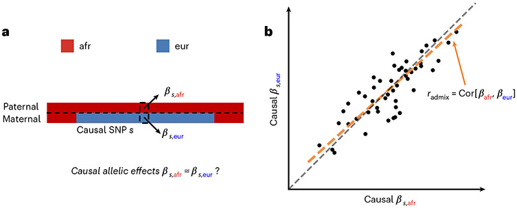
Our goal is to estimate the similarity in the causal effects across local ancestries in admixed populations (Fig. 1); the similarity can be evaluated across all genome-wide causal SNPs that are common across ancestries in a form of cross-ancestry genetic correlation^5,8 (for consistency with previous works we use ‘genetic correlation’ to refer to correlation of genetic effects across ancestries): ${\beta }_{s,\text{afr}}$, ${\beta }_{s,\text{eur}}$ are modeled as random variables following a bivariate Gaussian distribution parametrized by ${\sigma }_g^2$, ${\rho }_g$, denoting the variance and covariance of the effects:

$$\left[\begin{array}{c}\hfill {\beta }_{s,\text{afr}}\hfill \\ \hfill {\beta }_{s,\text{eur}}\hfill \end{array}\right]\sim N\left(\left[\begin{array}{c}\hfill 0\hfill \\ \hfill 0\hfill \end{array}\right],{\tau }_s^2\cdot \left[\begin{array}{c}\hfill \frac{{\sigma }_g^2}{S}\frac{{\rho }_g}{S}\hfill \\ \hfill \frac{{\rho }_g}{S}\frac{{\sigma }_g^2}{S}\hfill \end{array}\right]\right),s=1,\dots ,S,$$ (2)

where ${\tau }_s$ are variant-specific parameters determined by the genetic architecture assumption (Methods). Under this model, the genome-wide causal effects correlation is defined as $r_{\text{admix}}≔\frac{{\rho }_g}{{\sigma }_g^2};r_{\text{admix}}=1$ indicates same causal effects across local ancestries, while $r_{\text{admix}}<1$ indicates differences across ancestries. To estimate $r_{\text{admix}}$, given the genotype and phenotype data for a trait, we calculate the profile likelihood curve of $r_{\text{admix}}$, obtained by maximizing the likelihood of model defined by equations (1) and (2) with regard to parameters ${\sigma }_g^2$ and environmental variance for each fixed $r_{\text{admix}}\in [0,1]$. We assume $r_{\text{admix}}>0$ a priori both because causal effects are unlikely to be negatively correlated across ancestries and to reduce $r_{\text{admix}}$ search space for reducing computational cost; we have also performed real data analyses to verify this assumption (see below). We obtain the point estimate, credible interval and perform hypothesis testing $H_0:r_{\text{admix}}=1$ either for each individual trait using the trait-specific profile likelihood curve, or for meta-analysis across multiple traits using the multiplication of the likelihood curves across multiple traits (analogous to inverse variance weighted meta-analysis; Methods).

Fig. 1 ∣. Concepts of estimating similarity in the causal effects across local ancestries.

a, For a given trait, with phased genotype (paternal haplotype at the top and maternal haplotype at the bottom) and inferred local ancestry (denoted by color), we investigate whether ${\beta }_{s,\text{afr}}\approx {\beta }_{s,\text{eur}}$ across each causal SNPs. b, We focus on estimating the genome-wide correlation of genetic effects across ancestries $r_{\text{admix}}=\text{Cor}[{\beta }_{\text{afr}},{\beta }_{\text{eur}}]$, which is the regression slope (orange line) of ancestry-specific causal effects. For reference, the gray dashed line corresponds ${\beta }_{\text{afr}}={\beta }_{\text{eur}}$.

We organize next sections as follows. First, we show that our proposed approach provides accurate estimation of $r_{\text{admix}}$ in extensive simulations. Second, we show $r_{\text{admix}}$ is very close to 1 in real data of African-European admixed individuals from PAGE, UKBB and AoU. Third, we replicate our findings using methods that use GWAS summary data (marginal SNP effects at GWAS significant loci). Finally, we investigate pitfalls of methods^4,14,15,28 that use marginal SNP effects showing inflated heterogeneity; we find that Deming regression is the only approach robust enough to quantify $r_{\text{admix}}$ from marginal GWAS effects in admixed individuals.

Polygenic method for ${\mathit{r}}_{\mathbf{admix}}$ is accurate in simulations

We performed simulations to evaluate our proposed polygenic method using real genome-wide genotypes. We simulated phenotypes using genotypes and inferred local ancestries with N = 17,299 individuals and $S=6.9$ million SNPs (with MAF >0.5% in both ancestries in PAGE dataset; we omitted population-specific rare SNPs to reduce estimation variance; Methods). Phenotypes were simulated under a range of genetic architectures with a frequency-dependent causal effects distribution^29,30, and varying proportion of causal variants $P_{\text{causal}}$, heritability $h_g^2$ and true $r_{\text{admix}}$ (Methods). We used $P_{\text{causal}}=0.1\%$ in our main simulations (to simulate a typical polygenic complex trait³¹). When estimating $r_{\text{admix}}$, we either used all SNPs in the imputed genotypes that were used to simulate phenotypes, or restricted to HapMap3 (HM3) SNPs³² to simulate scenarios where causal variants are not perfectly typed in the data (Methods).

Our method produced accurate point estimates and well-calibrated credible intervals of $r_{\text{admix}}$ across a range of simulation settings (Fig. 2a and Supplementary Tables 1 and 2). We first evaluated our method in simulations with a realistic range of $h_g^2=0.1$, 0.25 and 0.5 and $r_{\text{admix}}=0.9$, 0.95 and 1.0. When using the imputed SNPs for estimation, results were approximately unbiased (average and maximal relative biases across simulation settings were −0.42% and −1.8% respectively). Credible intervals of $r_{\text{admix}}$ meta-analyzed across simulations approximately cover true $r_{\text{admix}}$: for the most biased setting ($h_g^2=0.1$, $P_{\text{causal}}=0.1\%$, $r_{\text{admix}}=0.95$), 95% credible interval 0.915–0.948. When using the HM3 SNPs for estimation, there was a consistent but small downward bias (Fig. 2a; average and maximal relative biases were −1.0% and −2.0%, respectively). This small downward bias was due to imperfect tagging that some of the causal SNPs were not included in the HM3 SNPs. Nonetheless, the magnitude of bias using either imputed or HM3 SNPs was small, indicating our method was accurate and robust to imperfect tagging. We next performed simulations to investigate the potential bias in estimating $r_{\text{admix}}$ due to omitting population-specific rare variants. We re-applied our methods using SNPs with MAF >1% and MAF >5% in both populations (in addition to the default MAF >0.5%) to the same simulated data. We observed downward bias in estimated $r_{\text{admix}}$ as more stringent MAF threshold was used and more SNPs were filtered out in estimation procedure. For example, the mode of the estimation was 0.966 when methods were applied with MAF >5% in simulation of $r_{\text{admix}}=1.0$ (Fig. 2b and Supplementary Table 3). This indicates omitting population-specific rare variants can lead to downward bias (Discussion). We also investigated the impact of prior assumption of $r_{\text{admix}}$: we applied a revised methodology that allows for $-1\le r_{\text{admix}}\le 1$ and we found that estimated $r_{\text{admix}}$ were highly consistent when assuming $0\le r_{\text{admix}}\le 1$ (default method) versus when assuming $-1\le r_{\text{admix}}\le 1$ (Fig. 2c).

Fig. 2 ∣. Results of genetic correlation ${\mathit{r}}_{\mathbf{admix}}$ estimation in genome-wide simulations.

Simulations were based on 17,299 PAGE individuals and 6.9 million genome-wide imputed variants with MAF > 0.5% in both ancestries. We fixed the proportion of causal variants $P_{\text{causal}}$ as 0.1% and varied genetic correlation $r_{\text{admix}}=0.90,0.95$ and 1.0. a, Impact of using HapMap3 or imputed variants in estimation. We varied simulated genome-wide heritability $h_g^2=0.1,0.25$ and 0.5. b, Impact of selecting common variants at different MAF thresholds in estimation. $h_g^2$ was fixed to 0.25, and imputed variants at different MAF thresholds were used in estimation. c, Impact of prior assumption in estimation. $h_g^2$ was fixed to 0.25, and imputed variants were used in estimation. For each simulated genetic architecture, we plot the mode and 95% credible interval based on the meta-analysis across 100 simulations (Methods). Numerical results are reported in Supplementary Tables 1-4 (including results for other $P_{\text{causal}}$, $r_{\text{admix}}$).

We performed several secondary analyses. We determined our method remained accurate at other simulated $P_{\text{causal}}$ (Supplementary Table 2; $P_{\text{causal}}$ ranging from 0.001% to 1%) and broader range of simulated $r_{\text{admix}}$ (Supplementary Table 4; $r_{\text{admix}}$ ranging from −0.5 to 1). In null simulations $(r_{\text{admix}}=1)$, we determined the false positive rate of hypothesis test $H_0:r_{\text{admix}}=1$ was properly controlled for most simulation settings, and was only slightly inflated when HM3 SNPs were used, and/or extremely low $P_{\text{causal}}$ was simulated. In simulations with $r_{\text{admix}}<1$, power to detect $r_{\text{admix}}<1$ increased with increasing $h_g^2$ and decreasing $r_{\text{admix}}$ (Supplementary Tables 1 and 2). In addition, we found heritability can be accurately estimated in these simulations (Supplementary Tables 5 and 6, and Methods). In summary, our method can be reliably used to estimate $r_{\text{admix}}$.

Causal effects are similar across local ancestries

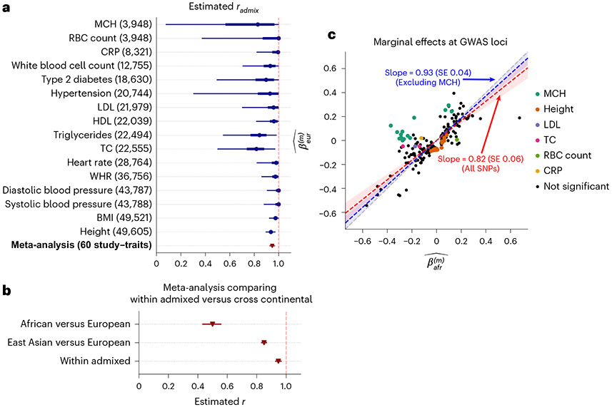
We applied our polygenic method to estimate $r_{\text{admix}}$ within African-European admixed individuals in PAGE¹ (24 traits, average N = 9,296, average fraction of African ancestries 78%), UKBB² (26 traits, average N = 3,808, average fraction of African ancestries 59%) and AoU³ (10 traits, average N = 20,496, average fraction of African ancestries 74%) (Methods). Meta-analyzing across 38 traits from PAGE, UKBB and AoU (60 study–trait pairs), we observed a high similarity in causal effects across ancestries (${\widehat{r}}_{\text{admix}}=0.95$, 95% credible interval 0.93–0.97). Results were highly consistent across datasets despite different ancestry compositions (PAGE: ${\widehat{r}}_{\text{admix}}=0.90$, 0.85–0.94; UKBB: ${\widehat{r}}_{\text{admix}}=0.98$, 0.91–1; AoU: ${\widehat{r}}_{\text{admix}}=0.97$, 0.94–1) as well as across traits (Fig. 3a, Table 1 and Supplementary Table 7). Height was the only trait that had significant ${\widehat{r}}_{\text{admix}}<1$ (after Bonferroni correction; nominal $P=4.3\times {10}^{-4}<0.05∕38$ ; meta-analyzed across three datasets; Table 1) albeit with high estimated ${\widehat{r}}_{\text{admix}}=0.936$, 0.89–0.97. Estimates of the same traits across datasets were only weakly correlated (Extended Data Fig. 1), suggesting similar causal effects by ancestry consistently across traits (true $r_{\text{admix}}\approx 1$ for all traits).

Fig. 3 ∣. Similarity of causal effects and marginal effects across local ancestries meta-analyzed across PAGE, UKBB and AoU.

a, We plot the trait-specific estimated $r_{\text{admix}}$ for 16 traits. For each trait, dots denote the estimation modes; bold lines and thin lines denote 50%/95% highest density credible intervals, respectively. Traits are ordered according to total number of individuals included in the estimation (shown in parentheses). These traits are selected to be displayed either because they have the largest total sample sizes, or because the associated SNPs of these traits exhibit heterogeneity in marginal effects (see the panel on the right). We also display the meta-analysis results across 60 study–trait pairs (38 unique traits). Numerical results are provided in Table 1. b, Comparison of $r_{\text{admix}}$ (n = 38 traits) to meta-analysis results from transcontinental genetic correlation of African versus European (n = 26 traits) and East Asian versus European (n = 31 traits). Point estimates and 95% confidence intervals are denoted using triangles and lines. c, We plot the ancestry-specific marginal effects for 217 GWAS significant clumped trait–SNP pairs across 60 study–trait pairs. Trait–SNP pairs with significant heterogeneity in marginal effects by ancestry ($p_{\mathsf{HET}}<0.05∕217$ via HET test) are denoted in color (non-significant trait–SNP pairs denoted as black dots; some black dots with large differences across ancestries were not significant because of the large standard errors in estimated effects). Numerical results are reported in Supplementary Table 11. Point estimates and 95% confidence intervals for Deming regression slopes of $\widehat{{\beta }_{s,\text{eur}}^{(m)}}\sim \widehat{{\beta }_{s,\text{afr}}^{(m)}}$ are provided either for all 217 SNPs (red), or for 193 SNPs after excluding 24 MCH-associated SNPs (blue). RBC, red blood cell; CRP, C-reactive protein; LDL, low-density lipoprotein cholesterol; HDL, high-density lipoprotein cholesterol; TC, total cholesterol; BMI, body mass index; WHR, waist-to-hip ratio.

Table 1 ∣.

Genome-wide genetic correlation across 38 complex traits for African-European admixed individuals in PAGE, UKBB and AoU

Trait	$N$	${\widehat{r}}_{\text{admix}}$ mode	95% credible interval(s)	$P$ value	$\widehat{h_g^2}$
BMD	1,668	0.000	0.00–0.78	0.012	0.34 ± 0.16
Neuroticism	3,044	1.000	0.36–1.00	1	0.36 ± 0.11
Education years	3,324	0.000	0.00–0.94	0.4	0.055 ± 0.075
MCHC	3,650	0.228	0.00–0.87	0.061	0.21 ± 0.092
Type 1 diabetes	3,767	0.381	0.00–0.95	0.77	−0.033 ± 0.016
HLR count	3,852	1.000	0.07–1.00	1	0.12 ± 0.086
RBC distribution width	3,925	1.000	0.27–1.00	1	0.28 ± 0.087
Lymphocyte count	3,935	1.000	0.00–0.60, 0.66–1.00	1	0.13 ± 0.086
Monocyte count	3,935	0.972	0.26–1.00	0.82	0.3 ± 0.087
MCH	3,948	0.829	0.07–1.00	0.36	0.2 ± 0.076
RBC count	3,948	1.000	0.37–1.00	1	0.31 ± 0.09
Hypothyroidism	4,063	1.000	0.05–1.00	1	0.046 ± 0.07
PR interval	4,071	0.844	0.08–1.00	0.36	0.22 ± 0.084
QRS interval	4,078	1.000	0.07–1.00	1	0.12 ± 0.082
Asthma	4,079	1.000	0.15–1.00	1	0.21 ± 0.087
Ever smoked	4,083	0.764	0.04–0.98	0.31	0.17 ± 0.082
QT interval	4,089	0.920	0.07–1.00	0.69	0.16 ± 0.083
HbA1c	5,353	0.954	0.08–1.00	0.77	0.19 ± 0.078
Cigarettes per day	6,995	0.999	0.08–1.00	1	0.097 ± 0.047
Fasting insulin	7,753	1.000	0.21–1.00	1	0.13 ± 0.044
eGFR	7,978	0.805	0.16–1.00	0.09	0.19 ± 0.046
C-reactive protein	8,321	0.995	0.82–1.00	0.94	0.28 ± 0.046
Fasting glucose	9,646	0.695	0.00–0.93	0.27	0.064 ± 0.035
Coffee consumption	11,587	0.982	0.10–1.00	0.9	0.074 ± 0.0 3
Platelet count	12,545	0.783	0.20–0.98	0.025	0.19 ± 0.038
White blood cell count	12,755	0.931	0.70–1.00	0.26	0.23 ± 0.036
Type 2 diabetes	18,630	0.897	0.49–1.00	0.23	0.12 ± 0.024
Hypertension	20,744	0.929	0.30–1.00	0.45	0.08 ± 0.027
LDL	21,979	0.958	0.70–1.00	0.55	0.14 ± 0.046
HDL	22,039	0.961	0.82–1.00	0.46	0.22 ± 0.057
Triglycerides	22,494	0.843	0.54–0.98	0.012	0.18 ± 0.027
Total cholesterol	22,555	0.818	0.50–0.97	0.007	0.18 ± 0.039
Heart rate	28,764	0.980	0.82–1.00	0.74	0.099 ± 0.015
WHR	36,756	0.973	0.86–1.00	0.55	0.12 ± 0.015
Diastolic blood pressure	43,787	1.000	0.90–1.00	1	0.077 ± 0.024
Systolic blood pressure	43,788	1.000	0.88–1.00	1	0.071 ± 0.013
BMI	49,521	0.974	0.92–1.00	0.33	0.22 ± 0.02
Height	49,605	0.936	0.89–0.97	0.00043	0.4 ± 0.014
Meta-analysis		0.947	0.93–0.97	8.7 × 10−7

For each trait, we report number of individuals, posterior mode and 95% credible interval(s) for estimated $r_{\text{admix}}$, nominal one-sided $P$ value for rejecting the null hypothesis of $H_0:r_{\text{admix}}=1$ (unadjusted for multiple testing; Methods), and estimated heritability and standard error. Meta-analysis results performed across 38 traits are shown in the last row. Traits are ordered according to number of individuals. For each trait, we perform meta-analysis across studies if the trait is in multiple studies (Methods). Lymphocyte count has two credible intervals because of the non-concave profile likelihood curve, as a result of small sample size. BMD, bone mineral density; HLR, high light scattering reticulocytes; MCHC, mean corpuscular hemoglobin concentration.

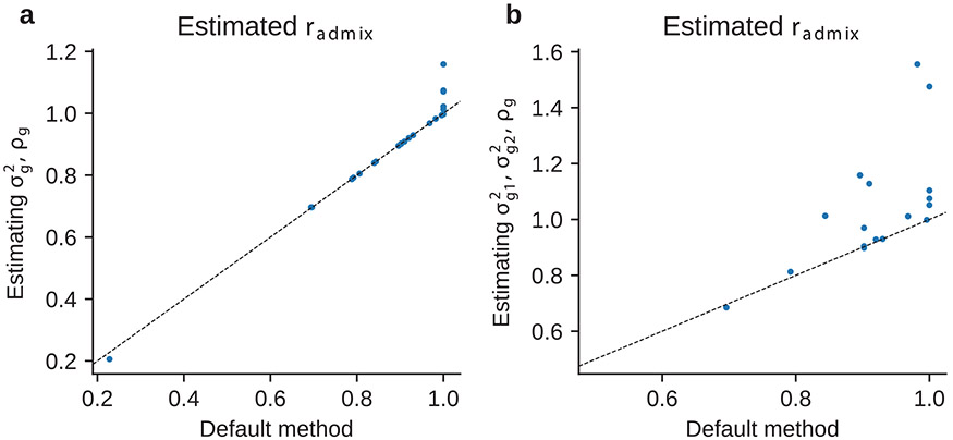
We performed several secondary analyses. Similar to previous simulation studies, we determined prior assumption of $r_{\text{admix}}$ had minimal impact to results: estimated $r_{\text{admix}}$ of 24 traits in PAGE were highly consistent when assuming $0\le r_{\text{admix}}\le 1$(default method) versus when assuming $-1\le r_{\text{admix}}\le 1$ (Extended Data Fig. 2). Such consistency between the two methods again indicates similar genetic causal effects across local ancestries $(r_{\text{admix}}\approx 1)$ and that estimation is robust to choices of statistical prior on $r_{\text{admix}}$. Our results were robust to different assumption of effects distribution (Extended Data Fig. 3 and Supplementary Table 8), consistent with previous work³³. Results were also robust to the SNP set used in the estimation (Extended Data Fig. 3 and Supplementary Table 8), and criterion of the included admixed individuals (Extended Data Fig. 4). Additionally, an alternative formulation of method assuming different variance component by ancestry did not outperform our default method assuming same variance component by ancestry (Extended Data Fig. 5, Supplementary Table 9 and Supplementary Note).

Next, we contrasted $r_{\text{admix}}$ to transcontinental genetic correlations of (1) European versus African and (2) European versus East Asian (Fig. 3b and Methods). We determine a much higher similarity across local ancestries within admixed populations (${\widehat{r}}_{\text{admix}}=0.95$, 95% credible interval 0.93–0.97) as compared with transcontinental correlations of African versus European within UKBB (${\widehat{r}}_{\text{eur}-\text{afr}}=0.50$, meta-analysis across 26 traits, 95% confidence interval 0.43–0.56) and East Asian (Biobank Japan) versus European (UKBB)⁸ (${\widehat{r}}_{\text{eur}-\text{eas}}=0.85$, meta-analysis across 31 traits, 95% confidence interval 0.83–0.87) (Supplementary Table 10). Overall, our results are consistent with $r_{\text{admix}}$ being less susceptible to heterogeneity due to differences in phenotyping/environment in transcontinental comparisons.

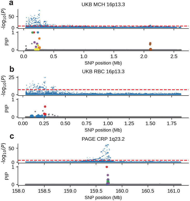
We sought to replicate high $r_{\text{admix}}$ using regression-based methods that leverage estimated ancestry-specific marginal effects at GWAS loci (Methods). Specifically, we used the following marginal regression equation (restricting equation (1) to each GWAS SNP $s$): $y=g_{s,\text{eur}}{\beta }_{s,\text{eur}}^{(m)}+g_{s,\text{afr}}{\beta }_{s,\text{afr}}^{(m)}+{\mathbf{c}}^{\mathsf{T}}\alpha +ϵ$ (we distinguish marginal effects ${\beta }^{(m)}$ from causal effects $\beta$; Methods). Across 60 study–trait pairs, we detected 217 GWAS significant clumped trait–SNP pairs and we estimated the ancestry-specific marginal effects for each SNP (Fig. 3c and Supplementary Table 11). We determined the estimated marginal effects are largely consistent by local ancestry at these GWAS clumped SNPs via Deming regression slope³⁴ of 0.82 (standard error 0.06) (applied to $\widehat{{\beta }_{s,\text{eur}}^{(m)}}\sim \widehat{{\beta }_{s,\text{afr}}^{(m)}}$; Deming regression properly accounts for uncertainty in both dependent and independent variables; Methods). Mean corpuscular hemoglobin (MCH)-associated SNPs at 16p13.3 drove most of the differences by ancestry: Deming regression slope was 0.93 (standard error 0.04) on the rest of 193 SNPs after excluding 24 MCH-associated SNPs; MCH-associated SNPs also have the strongest heterogeneity in marginal effects by ancestry (using heterogeneity score test (HET) for testing effects heterogeneity at each SNP³⁵; Supplementary Table 11 and Methods). By performing statistical fine-mapping analysis, we found there are multiple conditionally independent association signals at MCH-associated and other loci with heterogeneity by ancestry (Extended Data Fig. 6 and Supplementary Note). In fact, the MCH-associated loci locate at a region harboring alpha-globin gene cluster (HBZ–HBM–HBA2–HBA1–HBQ1) known to contain multiple causal variants³⁶. These results suggest that, similar to causal effects, marginal effects at GWAS loci are also largely consistent by local ancestry across multiple traits, with the exception of 16p13.3 loci for MCH in our study, where multiple large-effect causal variants drive some extent of heterogeneity by ancestry in marginal effects.

Pitfalls of using marginal effects to estimate heterogeneity

Next, we focused on thoroughly evaluating methods that use marginal effects at GWAS significant variants to estimate heterogeneity. Marginal effects are frequently used to compare effect sizes across populations or across studies^4,14,15,28 and enjoy popularity for their simplicity and requirement of only GWAS summary statistics (estimated effect sizes and standard errors).

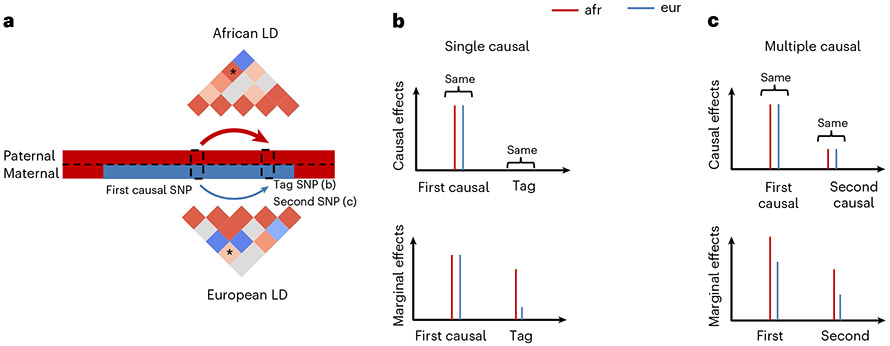
We first note that heterogeneities in marginal effects can be induced due to different LD patterns across ancestries even when the underlying causal effects are identical, especially when multiple causal variants are nearby in the same LD block (Fig. 4). We investigate the extent of heterogeneity by ancestry that can be induced in simulations with identical causal effects across ancestries, due to (1) local ancestry adjustment; (2) unknown causal variants coupled with ancestry-specific LD patterns; (3) highly polygenic genetic architectures with multiple causal SNPs within the same LD block; (4) standard errors in estimated marginal effects across ancestries. Our following simulations were based on real imputed genotypes from African-European individuals in PAGE data (17,299 individuals, average fraction of African ancestries 78%).

Fig. 4 ∣. Induced heterogeneities in marginal effects across local ancestries.

a, Illustrations that different LD patterns across local ancestries can induce differential tagging between a causal SNP and a tag SNP in b or another causal SNP in c. LD strengths between the two SNPs are indicated both in the thickness of arrows and in the color shades of ‘*’ elements in LD matrices. b, Example of single causal SNP with no heterogeneity. Causal effects are the same across local ancestries, and the estimated marginal effects at causal SNP will be also very similar with sufficient sample size. However, because of differential tagging across local ancestries, the estimated marginal effects evaluated at the tag SNP are difference. c, Example of multiple causal SNPs with no heterogeneity. Causal effects for both SNPs are the same across local ancestries. In this example, the correlation between the two causal variants is higher for genotypes in African local ancestries than those in European local ancestries. Therefore, African ancestry-specific genotypes tag more effects, creating different ancestry-specific marginal effects at each causal SNP.

Regressing out local ancestry can deflate the observed similarity in causal effects across ancestries.

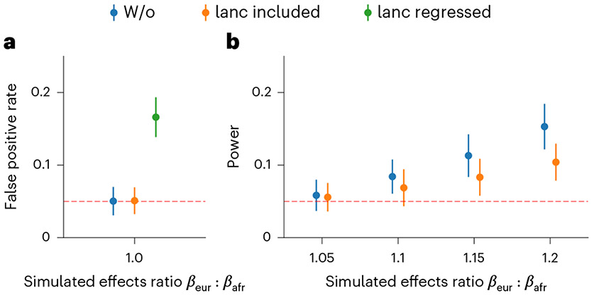
We first discuss the use of local ancestry in the heterogeneity estimation, which is a unique and important component to consider when studying admixed populations. We used simulations to investigate the role of local ancestry adjustment using three main approaches: (1) ignoring local ancestry altogether (‘w/o’); (2) including local ancestry as covariate in the model (‘lanc-included’); (3) regressing out the local ancestry from phenotype followed by heterogeneity estimation on residuals (‘lanc-regressed’) (Methods). First, in null simulations with identical causal effects (ratio of ${\beta }_{\text{eur}}:{\beta }_{\text{afr}}=1$), we observed that ignoring local ancestry or including local ancestry as covariate yielded well-calibrated HET tests; in contrast, regressing out the local ancestry effect induced inflated HET test statistics (Fig. 5 and Supplementary Table 12). Next, in power simulations with varying amount of heterogeneity (defined as ratio of ${\beta }_{\text{eur}}:{\beta }_{\text{afr}}$), including local ancestry in the covariate significantly reduced the power of HET test of up to 50% at high magnitude of heterogeneity (Fig. 5 and Supplementary Table 12) (see more details in Supplementary Note). Thus, with respect to local ancestry, we recommend either not using it or including it as a covariate in the model and not regressing out its effect before heterogeneity estimation as that will bias heterogeneity estimation.

Fig. 5 ∣. Pitfalls of including local ancestry in estimating heterogeneity.

In each simulation, we selected a single causal variant and simulated quantitative phenotypes where these causal variants explain heritability $h_g^2=0.6\%$; we also varied ratios of effects across ancestries ${\beta }_{\text{eur}}:{\beta }_{\text{afr}}$. a, False positive rate in null simulation ${\beta }_{\text{eur}}:{\beta }_{\text{afr}}=1.0$. b, Power to detect ${\beta }_{\text{eur}}\ne {\beta }_{\text{afr}}$ in power simulations with ${\beta }_{\text{eur}}:{\beta }_{\text{afr}}>1$. We did not include ‘lanc regressed’ because it is not well-calibrated in null simulations. We plot the mean and 95% confidence intervals, calculated via 100 random subsamplings with each sample consisting of 500 SNPs (Methods). Numerical results are reported in Supplementary Table 12.

Having investigated the role of local ancestry adjustment, we next turn to heterogeneity estimation for GWAS SNPs. We focused on investigating properties of HET test and Deming regression in null simulations with identical causal effects across ancestries ${\beta }_{\text{eur}}:{\beta }_{\text{afr}}=1$. Since the true causal variants are usually uncertain, we investigated each method either at the true simulated causal variants or at the LD-clumped variants (Methods).

Uncertainty in which variants are causal can deflate the observed similarity in effects by ancestry.

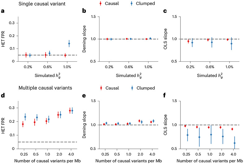
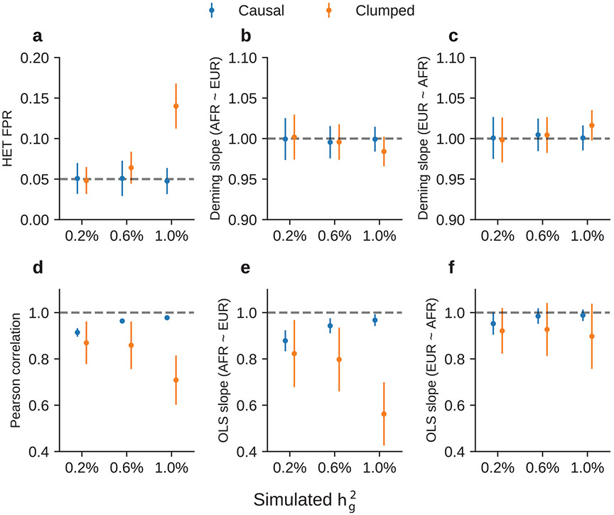
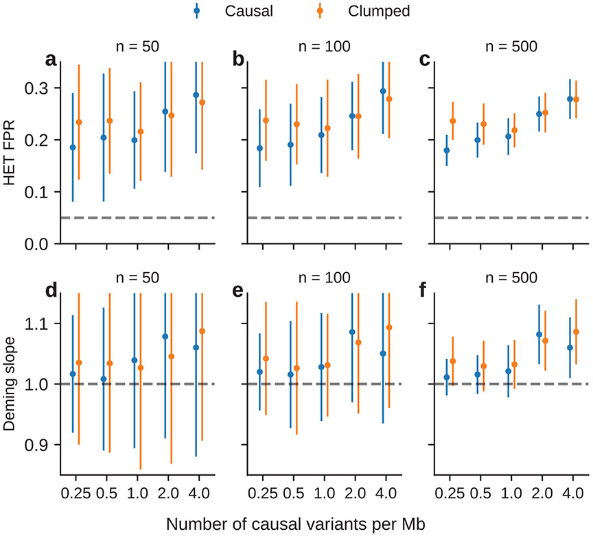
We first performed simulations with single causal variant: we randomly selected one SNP as causal in each simulation. Evaluated at the causal SNPs (Methods), we found that HET test and Deming slope were well-calibrated (Fig. 6a-c, Extended Data Fig. 7 and Supplementary Table 13). However, evaluated at the clumped variants, as a more realistic setting (because causal variants need to be inferred), we found HET test became increasingly miscalibrated with increased $h_g^2$, while Deming slope remained relatively robust (with an upward but not statistically significant trend with increasing $h_g^2$). Ordinary least squares (OLS) slope had bias even when evaluated at causal variants because of its ignorance of the standard errors in the estimated effects (Methods and Supplementary Note); such bias became smaller with increased $h_g^2$.

Fig. 6 ∣. Miscalibration of HET test/Deming regression/OLS regression in simulations with ${\mathit{r}}_{\text{admix}}=1$.

a–c, Simulations with single causal variant. Each causal variant had the same causal effects across local ancestries and each causal variant explained a fixed amount of heritability (0.2%, 0.6% and 1.0%): false positive rate (FPR) of HET test (a); Deming regression slope (b) and of OLS regression slope (c) of $\widehat{{\beta }_{\text{eur}}^{(m)}}\sim \widehat{{\beta }_{\text{afr}}^{(m)}}$. Numerical results are reported in Supplementary Table 13. d–f, Simulation with multiple causal variants, where we simulated different levels of polygenicity, such that on average there were approximately 0.25, 0.5, 1.0, 2.0 and 4.0 causal variants per Mb; causal variants had the same causal effects across local ancestries, and the heritability explained by all causal variants was fixed at $h_g^2=10\%$: FPR of HET test (d); Deming regression slope (e) and OLS regression slope (f) of $\widehat{{\beta }_{\text{eur}}^{(m)}}\sim \widehat{{\beta }_{\text{afr}}^{(m)}}$. The 95% confidence intervals were based on 100 random subsamplings with each sample consisting of 1,000 SNPs (Methods). Results for other number of SNPs used for subsampling are shown in Extended Data Fig. 8. Numerical results are reported in Supplementary Table 14.

High polygenicity can deflate the observed similarity in effects by ancestry.

Next, we performed simulations where multiple causal variants locate nearby within the same LD block (typical for polygenic complex traits^37,38; Methods). In this scenario, marginal GWAS effects could tag multiple causal effects, thus potentially inflating the observed heterogeneity (Fig. 4c). In simulations, we varied the number of causal SNPs from 0.25 to 4.0 per Mb to span most polygenic architectures. In contrast to simulations with a single causal variant, all three methods (HET test, Deming slope and OLS slope) were biased in the presence of multiple nearby causal variants; the miscalibration/bias increased with number of causal variants per region, and LD clumping did not alleviate the miscalibration/bias (Fig. 6d-f). Such miscalibrations occurred irrespective of sample size (Extended Data Fig. 8), or simulated heritability $h_g^2$ (Supplementary Table 14).

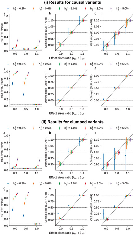
In summary, we find that methods for heterogeneity-by-ancestry estimation based on marginal GWAS SNP effects are susceptible to inflated estimates of heterogeneity. HET test is susceptible to false positives when causal variants are unknown. Deming regression was robust in scenarios with low polygenicity, but was still susceptible to inflated estimates of heterogeneity for highly polygenic traits; the inflated estimates can be explained by differential tagging of causal effects across ancestries among causal SNPs. OLS slope had bias because it did not account for uncertainty in estimated effects. We also performed additional simulations with less than identical causal effects ${\beta }_{\text{eur}}:{\beta }_{\text{afr}}\ne 1$ and broader range of per-SNP $h_g^2$ and we determined Deming regression was robust to quantify the heterogeneity level at the marginal effects in simulations of different ${\beta }_{\text{eur}}:{\beta }_{\text{afr}}$, $h_g^2$ (Extended Data Fig. 9 and Supplementary Table 15).

Discussion

In this work, we developed a polygenic method that model genome-wide causal effects to complex traits of admixed individuals. We determined causal effects are largely similar across local ancestries in analysis of 53,001 African-European admixed individuals across 38 complex traits in PAGE, UKBB and AoU. In addition to causal effects, we also replicated such consistency-by-ancestry for marginal effects at GWAS loci. We highlighted realistic simulation scenarios where regression-based methods using marginal effects can report false heterogeneity when causal effects are identical across ancestries.

Our study has several implications for future genetic study of admixed populations, and more broadly of ancestrally diverse individuals. First, reduced accuracy of polygenic score has been observed in African-European admixed populations with increasing proportion of non-European ancestries²¹; our results suggest the causal effects difference has limited contribution to such reduced accuracy. Second, there has been recent work on incorporating local ancestry in statistical modeling of admixed populations, for example, in association testing¹⁹ and polygenic score^21,22, based on the hypothesis that effects may differ across ancestries. Our results indicate the largely consistent causal effects across local ancestries (and also marginal effects at most GWAS loci). The robustness of our results to imperfect tagging also suggests that imperfect tagging induce limited effects heterogeneity across local ancestries, once SNPs are properly modeled in a polygenic model. The small heterogeneity-by-ancestry at causal effects or marginal effects suggest that association tests that do not model heterogeneity-by-ancestry should be preferred in most cases^19,20 for improved statistical power for association. On the other hand, including local ancestry in association models could be useful in correcting for LD induced by admixture³⁹ and lead to improved causal effect estimation. Full consideration of incorporating local ancestry in statistical models should also take into account the extent of confounding and heterogeneity in the data⁴⁰. Third, our study further motivates studies of ancestrally diverse individuals to identify population-specific risk variants that cannot be investigated due to being rare in European individuals; for example, inclusion of individuals with diverse populations could further disentangle causal from tagging effects, thus increasing the power of heterogeneity-by-ancestry estimation. More importantly, larger and robust trans-ancestry studies may allow for the examination of differential causal effects on a locus-by-locus basis, in addition to the genome-wide approach as presented in this work.

Our results add to the existing literature to further delineate sources of causal effects differences. Previous works have shown moderate causal effects differences across transcontinental populations^5,6,8,28, with part of differences being induced by heterogeneity in the definition of environment/phenotype across continental ancestries. Similarly, a recent work¹⁵ concluded differences between causal effects in European local ancestries within African American admixed individuals and that in European American individuals. Our results showcase that, if environments are well controlled (as is the case for genetic variants across local ancestries within admixed populations), causal effects are highly similar across genetic ancestries, agreeing with a recent study finding similar effects across ancestries at level of gene expression in controlled environments⁴¹. Moreover, our results suggest that local epistatic interaction, if any, does not lead to large causal effects differences across genetic ancestries. By contrasting the high genetic correlation within admixed populations and the low genetic correlation across continental populations, our results support the hypothesis that different environments modify the genetic effects to complex traits (gene-by-environment interaction) across populations.

We note several limitations and future directions of our work. First, we have analyzed SNPs with MAF ≥0.5% in both ancestries. We excluded population-specific SNPs (with MAF <0.5% in one of the ancestries) because these SNPs provide little information for estimating $r_{\text{admix}}$, since effects for these SNPs are estimated with large noises. We used simulations to show that omitting these rare variants could lead to downward bias in $r_{\text{admix}}$ estimation because of population-specific tagging of shared causal variants (Supplementary Note). However, it remains possible that causal variants themselves are rare and population-specific, and upward bias in the estimation of $r_{\text{admix}}$ may be present. While in this work we focused on estimating $r_{\text{admix}}$ for common variants, future work with larger sample sizes is needed to further investigate the impact of population-specific causal SNPs to $r_{\text{admix}}$ estimation. Second, we have considered two-way African-European admixed individuals. Several practical considerations remain before applying this method to other admixed populations such as three-way admixture: local ancestries are typically inferred with larger errors⁴², and this should be accounted for in statistical modeling (it may be possible to incorporate posterior probabilities in estimated local ancestries to obtain calibrated estimates); additional parameters need to be estimated (for example, three pairwise correlation parameters across ancestries for three-way admixture populations). We note that our methods can be readily applied to these populations when reliable local ancestry calls can be obtained. Third, our modeling can be extended to estimate correlations in causal effects stratified by functional annotation categories and we leave that as future work. Fourth, our polygenic method requires individual-level genotype and phenotype; if not available, we found Deming regression may be applied to evaluate heterogeneity with caution: in our simulation, Deming regression was the only method robust to most scenarios except for high polygenicity. In our analysis of marginal effects, we found LD clumping can produce cluster of SNPs that were nearby and probably dependent with each other, as a combined result of multiple causal variants within a region and long-range LD in admixed populations. Such dependence may induce bias for methods like Deming regression, highlighting the need for improved methods of identifying conditionally independent SNPs in admixed populations. Fifth, we have meta-analyzed three publicly available studies of PAGE, UKBB and AoU with large cohort of African-European admixed individuals. Such meta-analysis with greatly increased total sample size enabled us to derive the conclusion of the high similarity in causal effects by local ancestry across a broad range of traits. However, our estimates for each individual trait were still associated with large standard errors and can be further improved by analyzing more individuals. Additional limitations are discussed in Supplementary Note. Despite these limitations, our study has shown that causal effects to complex traits are highly similar across local ancestries, and this knowledge can be used to guide future genetic studies of ancestrally diverse populations.

Methods

Ethical approval

This research complies with all relevant ethical regulations. Ethics committee/institutional review board (IRB) of PAGE gave ethical approval for collection of PAGE data. Ethics committee/IRB of UKBB gave ethical approval for collection of UKBB data (https://www.ukbiobank.ac.uk/learn-more-about-uk-biobank/about-us/ethics). Approval to use UKBB individual level in this work was obtained under application 33297 at http://www.ukbiobank.ac.uk. Ethics committee/IRB of AoU gave ethical approval for collection of AoU data (https://allofus.nih.gov/about/who-we-are/institutional-review-board-irb-of-all-of-us-research-program). Approval to use AoU controlled tier data in this work was obtained through application at https://www.researchallofus.org.

Statistical model of phenotype for admixed individuals

For individual $i=1,\dots ,N$ and SNP $s=1,\dots ,S$, we denote $x_{i,s,M}$, $x_{i,s,P}$ as number of minor alleles at maternal and paternal haplotypes, respectively. We denote corresponding local ancestries as ${\gamma }_{i,s,M},{\gamma }_{i,s,P}\in \{1,2\}$ (we focus on two-way admixture here, for example, ‘1’ and ‘2’ denote African and European ancestries for African-European admixture). Then we use $g_{i,s,1}$, $g_{i,s,2}$ to encode allele counts that are specific to each local ancestry:

$$\begin{gathered} g_{i,s,1}≔x_{i,s,M}\mathbb{I}\left({\gamma }_{i,s,M}=1\right)+x_{i,s,P}\mathbb{I}\left({\gamma }_{i,s,P}=1\right); \\ {g}_{i,s,2}≔x_{i,s,M}\mathbb{I}\left({\gamma }_{i,s,M}=2\right)+x_{i,s,P}\mathbb{I}\left({\gamma }_{i,s,P}=2\right), \end{gathered}$$

where $\mathbb{I}(\cdot )$ denotes the indicator function. Denoting causal allelic effects as ${\beta }_1$, ${\beta }_2\in {\mathbb{R}}^S$ for two ancestries, we model the phenotype of each individual $y_i$ as

$$y_i={\mathbf{c}}_i^{\mathsf{T}}\alpha +\sum _{s=1}^S(g_{i,s,1}{\beta }_{s,1}+g_{i,s,2}{\beta }_{s,2})+{ϵ}_i,i=1,\dots ,N$$

where ${\mathbf{c}}_i\in {\mathbb{R}}^C$, $\alpha \in {\mathbb{R}}^C$ denote $C$ covariates (including all ‘1’ intercepts) and their effects. ${ϵ}_i$ denotes environmental noise. By further aggregating $g_{i,s,1}$, $g_{i,s,2}$ into matrices ${\mathbf{G}}_1\in {\{0,1,2\}}^{N\times S}$ and ${\mathbf{G}}_2\in {\{0,1,2\}}^{N\times S}$ for ancestry 1 and 2, and ${\mathbf{c}}_i$ into $\mathbf{C}\in {\mathbb{R}}^{N\times C}$, equation (1) becomes

$$\mathbf{y}=\mathbf{C}\alpha +{\mathbf{G}}_1{\beta }_1+{\mathbf{G}}_2{\beta }_2+ϵ$$ (3)

We pose the following distribution assumptions ${\beta }_1$, ${\beta }_2$ and $ϵ$

$$\left[\begin{array}{c}\hfill {\beta }_{s,1}\hfill \\ \hfill {\beta }_{s,2}\hfill \end{array}\right[\sim N\left(\left[\begin{array}{c}\hfill 0\hfill \\ \hfill 0\hfill \end{array}\right],{\tau }_s^2\cdot \left[\begin{array}{cc}\hfill {\sigma }_g^2∕S\hfill & \hfill {\rho }_g∕S\hfill \\ \hfill {\rho }_g∕S\hfill & \hfill {\sigma }_g^2∕S\hfill \end{array}\right]\right),s=1,\dots ,S,{ϵ}_i\sim N(0,{\sigma }_e^2),i=1,\dots ,N$$ (4)

where ${\sigma }_g^2$ denotes variance of effects for both populations, ${\rho }_g$ denotes covariance for similarity of effect sizes by ancestry, and ${\sigma }_e^2$ denotes the variance for environments. ${\tau }_s$ denote SNP-specific parameters (fixed a priori) for effect sizes distribution (see ‘Specifying τ_s under different heritability models‘ below). We define correlation of causal genetic effects as $r_{\text{admix}}=\frac{{\rho }_g}{{\sigma }_g^2}$. $r_{\text{admix}}=1$ indicates ${\beta }_{s,1}={\beta }_{s,2}$ for all variants $s=1,\dots ,S$, that is, causal effects are the same across ancestries; $r_{\text{admix}}<1$ indicates differences in causal effects across ancestries.

Calculating and filtering by ancestry-specific allele frequencies.

For each SNP $s$, we calculated MAF as $f_s≔\frac{{\sum }_{i=1}^N(g_{i,s,1}+g_{i,s,2})}{2N}$. We also calculated ancestry-specific MAF as $\frac{{\sum }_{i=1}^N(g_{i,s,1})}{{\sum }_{i=1}^N[\mathbb{I}({\gamma }_{i,s,M}=1)+\mathbb{I}({\gamma }_{i,s,P}=1)]},\frac{{\sum }_{i=1}^N(g_{i,s,2})}{{\sum }_{i=1}^N[\mathbb{I}({\gamma }_{i,s,M}=2)+\mathbb{I}({\gamma }_{i,s,P}=2)]}$ for ancestry 1 and 2. For a SNP $s$ with close-to-zero frequency for either of the ancestry, its effect ${\beta }_s$ will be estimated with very large noise. Therefore, we used SNPs with MAF >0.5% in both ancestries in analyses.

Specifying ${\tau }_{\mathit{s}}$ under different heritability models.

${\tau }_s$ parameters model the coupling of SNP effects variance with MAF, local LD or other functional annotations. Commonly used heritability models include GCTA⁴³, frequency-dependent^29,30, LDAK⁴⁴ and S-LDSC⁴⁵ models. While heritability model is important to estimate heritability and functional enrichment of heritability^33,46,47, genetic correlation estimation, the main focus of this study, has shown to be robust to different heritability models³³. In this work, we mainly used the frequency-dependent model for both simulations and real data analyses (where ${\tau }_s^2\propto {[f_s(1-f_s)]}^{\alpha };f_s$ is the MAF of the SNP $s$ and $\alpha =-0.38$ is estimated in a meta-analysis across 25 UKBB complex traits³⁰). For real data analysis, we additionally used GCTA model for estimation and found results are robust to heritability models (Extended Data Fig. 3).

Alternative choice of genotype normalization by ancestry.

We discuss an alternative choice of normalization by ancestry, in which we have two parameters ${\tau }_{s,1}$ and ${\tau }_{s,2}$ separately for two ancestries for each SNP. For example, ${\tau }_{s,1}^2\propto \frac{1}{f_{s,1}(1-f_{s,1})}$, ${\tau }_{s,2}^2\propto \frac{1}{f_{s,2}(1-f_{s,2})}$ parametrizing effects distribution

$$\left[\begin{array}{c}\hfill {\beta }_{s,1}\hfill \\ \hfill {\beta }_{s,2}\hfill \end{array}\right[\sim 𝒩\left(\left[\begin{array}{c}\hfill 0\hfill \\ \hfill 0\hfill \end{array}\right],\left[\begin{array}{cc}\hfill {\tau }_{s,1}^2\cdot {\sigma }_g^2∕S\hfill & \hfill {\tau }_{s,1}{\tau }_{s,2}\cdot {\rho }_g∕S\hfill \\ \hfill {\tau }_{s,1}{\tau }_{s,2}\cdot {\rho }_g∕S\hfill & \hfill {\tau }_{s,2}^2\cdot {\sigma }_g^2∕S\hfill \end{array}\right]\right),s=1,\dots ,S$$

This implies that effects per genotype standard deviation is being modeled (ref.⁵ termed this as correlation of allelic impact). While genetic correlation estimation is robust to genotype standardization (Supplementary Table 8; refs. ^5,33), we recommend modeling allelic effects via same ${\tau }_s$ across ancestries (as used in our default Methods).

Evaluation of genome-wide genetic effects consistency

We discuss parameter estimation and hypothesis testing in equations (3) and (4). Marginalizing over random effects ${\beta }_1$ and ${\beta }_2$ in equation (3), the distribution of $\mathbf{y}$ is

$$\mathbf{y}\sim N\left(\mathbf{C}\alpha ,{\sigma }_g^2\frac{{\mathbf{G}}_1\mathbf{T}{\mathbf{G}}_1^{\mathsf{T}}+{\mathbf{G}}_2\mathbf{T}{\mathbf{G}}_2^{\mathsf{T}}}{S}+{\rho }_g\frac{{\mathbf{G}}_1\mathbf{T}{\mathbf{G}}_2^{\mathsf{T}}+{\mathbf{G}}_2\mathbf{T}{\mathbf{G}}_1^{\mathsf{T}}}{S}+{\sigma }_e^2\mathbf{I}\right).$$

where $\mathbf{T}$ is a diagonal matrix with ${(\mathbf{T})}_{ss}={\tau }_s^2$. By denoting ${\mathbf{K}}_1=\frac{{\mathbf{G}}_1{\mathbf{TG}}_1^{⊺}+{\mathbf{G}}_2{\mathbf{TG}}_2^{⊺}}{S}$, ${\mathbf{K}}_2=\frac{{\mathbf{G}}_1{\mathbf{TG}}_2^{⊺}+{\mathbf{G}}_2{\mathbf{TG}}_1^{⊺}}{S}$, and ${\rho }_g={\sigma }_g^2\cdot r_{\text{admix}}$, the distribution of $\mathbf{y}$ is simplified as

$$y\sim N\left(\mathbf{C}\alpha ,{\sigma }_g^2({\mathbf{K}}_1+r_{\text{admix}}{\mathbf{K}}_2)+{\sigma }_e^2\mathbf{I}\right).$$ (5)

The maximum likelihood estimates of $(\alpha ,{\sigma }_g^2,r_{\text{admix}},{\sigma }_e^2)$ can be found by directly maximizing the corresponding likelihood function $L(\alpha ,{\sigma }_g^2,r_{\text{admix}},{\sigma }_e^2)$. However, the constraint that the correlation parameter $r_{\text{admix}}$ should be small than 1 cannot be easily incorporated here. Instead, we use the profile likelihood $L_p(r_{\text{admix}})≔\underset{(\alpha ,{\sigma }_g^2,{\sigma }_e^2)}{\max }L(\alpha ,{\sigma }_g^2,r_{\text{admix}},{\sigma }_e^2)$ and perform grid search of $r_{\text{admix}}$ to maximize profile likelihood (similar to ref.³⁰): for each candidate $r_{\text{admix}}$, we compute ${\mathbf{K}}_1+r_{\text{admix}}{\mathbf{K}}_2$, and solve $(\alpha ,{\sigma }_g^2,{\sigma }_e^2)$for the single variance component model in equation (5) using GCTA²⁷ (v1.94.0beta). In practice, we calculate profile likelihood $L_p(r_{\text{admix}})$ for a predefined set of $r_{\text{admix}}=0.00,0.05,\dots ,1.00(r_{\text{admix}}\in [0,1]$ is a reasonable prior assumption here; we alternatively used an extended range of $r_{\text{admix}}=-1,-0.95,\dots ,0.95,1.0$ in simulation studies (Supplementary Table 4) and real data analyses (Extended Data Fig. 2)). We use natural cubic spline to interpolate pairs of $(r_{\text{admix}},L_p(r_{\text{admix}}))$ to get a likelihood curve of $r_{\text{admix}}$. Then we obtain the estimated ${\widehat{r}}_{\text{admix}}$ using the value that maximize the likelihood curve, and credible interval by combining the likelihood curve with a uniform prior of $r_{\text{admix}}\sim \text{Uniform}[0,1]$ and calculating the highest posterior density interval as credible interval. To perform the meta-analysis across independent estimates, we obtain the joint likelihood by calculating the product of likelihood curves across estimates (or equivalently, the sum of log-likelihood curves), and similarly calculate the estimate and credible interval.

Evaluation of genetic effects consistency at individual variant with marginal effects

Parameter estimation and hypothesis testing.

We use a model between individual SNP and phenotype by restricting equation (1) to the SNP of interest $s$, as

$$y_i={\mathbf{c}}_i^{\mathsf{T}}\alpha +\left(g_{i,s,1}{\beta }_{s,1}^{(m)}+g_{i,s,2}{\beta }_{s,2}^{(m)}\right)+{ϵ}_i,i=1,\dots ,N,$$

or in vector form,

$$y=\mathbf{C}\alpha +{\mathbf{g}}_{s,1}{\beta }_{s,1}^{(m)}+{\mathbf{g}}_{s,2}{\beta }_{s,2}^{(m)}+ϵ$$ (6)

where $\mathbf{C}$, ${\mathbf{g}}_{s,1}$, ${\mathbf{g}}_{s,2}$, $ϵ$ contain ${\mathbf{c}}_i$, $g_{i,s,1}$, $g_{i,s,2}$, ${ϵ}_i$ for all individuals $i=1,\dots ,N$, respectively. We distinguish marginal effects ${\beta }_{s,1}^{(m)}$, ${\beta }_{s,2}^{(m)}$ in equation (6) from causal effects ${\beta }_{s,1}$, ${\beta }_{s,2}$ in Eq. (1): marginal effects tag effects from nearby causal SNPs with taggability as a function of ancestry-specific correlation between the focal SNP and nearby causal SNPs. Therefore, heterogeneity in marginal effects by local ancestry can be induced even if causal effects are the same (see extensive simulations in Results and more details in Supplementary Note). We estimate ${\beta }_{s,1}^{(m)}$, ${\beta }_{s,2}^{(m)}$ using least squares (jointly for ${\beta }_{s,1}^{(m)}$, ${\beta }_{s,2}^{(m)}$) and perform hypothesis testing of $H_0:{\beta }_{s,1}^{(m)}={\beta }_{s,2}^{(m)}$ with a likelihood ratio test by comparing Eq. (6) to a restricted model where the allelic effects are the same ${\beta }_s^{(m)}={\beta }_{s,1}^{(m)}={\beta }_{s,2}^{(m)}$:

$$y=\mathbf{C}\alpha +({\mathbf{g}}_{s,1}+{\mathbf{g}}_{s,2}){\beta }_s^{(m)}+ϵ$$ (7)

Marginal effects-based methods for estimating heterogeneity.

We describe details of marginal effects-based methods to estimate heterogeneity with input from a set of estimated effect sizes $\widehat{{\beta }_{s,1}^{(m)}}$, $\widehat{{\beta }_{s,2}^{(m)}}$ and corresponding estimated standard errors $\widehat{\text{se}({\beta }_{s,1}^{(m)})}$, $\widehat{\text{se}({\beta }_{s,2}^{(m)})}$ for a set of SNPs.

• Pearson correlation: by calculating the Pearson correlation of $\widehat{{\beta }_{s,1}^{(m)}}$, $\widehat{{\beta }_{s,2}^{(m)}}$ across SNPs. Pearson correlation does not model errors in estimated effects, therefore is expected be smaller than 1 and decreases with increasing error magnitude.

• OLS regression slope: by regressing $\widehat{{\beta }_{s,1}^{(m)}}\sim \widehat{{\beta }_{s,2}^{(m)}}$ ($\widehat{{\beta }_{s,1}^{(m)}}$ as dependent variable, $\widehat{{\beta }_{s,2}^{(m)}}$ as independent variable) or $\widehat{{\beta }_{s,2}^{(m)}}\sim \widehat{{\beta }_{s,1}^{(m)}}$. It does not model errors in independent variable. Moreover, it assumes homogeneous errors in dependent variable across SNPs. Therefore, it is susceptible to these error terms and notably results can vary when one exchange the regression orders⁴⁸ ($\widehat{{\beta }_{s,1}^{(m)}}\sim \widehat{{\beta }_{s,2}^{(m)}}$ versus $\widehat{{\beta }_{s,2}^{(m)}}\sim \widehat{{\beta }_{s,1}^{(m)}}$; for example, $\widehat{{\beta }_{s,1}^{(m)}}$ and $\widehat{{\beta }_{s,2}^{(m)}}$ are associated with different standard errors when being estimated in an admixed population with different ancestry proportion).

• Deming regression slope: obtained with Deming regression³⁴ of $\widehat{{\beta }_{s,1}^{(m)}}$, $\widehat{{\beta }_{s,2}^{(m)}}$ and estimated standard errors $\widehat{\text{se}({\beta }_{s,1}^{(m)})}$, $\widehat{\text{se}({\beta }_{s,2}^{(m)})}$. Deming regression models heterogeneous error terms in both independent and dependent variables, therefore is more robust than Pearson correlation and OLS regression. Specifically, given a set of data and estimated standard errors $(x_i,y_i,{\sigma }_{x,i},{\sigma }_{y,i}),i=1,\dots ,n$ (we use a different set of notations for simplicity), Deming regression optimizes the following objective function to obtain estimated intercept $\alpha$ and slope $\beta$:

$$\begin{gathered} \underset{\begin{array}{c}\hfill \alpha ,\beta \hfill \\ \hfill {\delta }_1,\dots ,{\delta }_n\hfill \\ \hfill {ϵ}_i,\dots ,{ϵ}_n\hfill \end{array}}{\text{min}}\sum _{i=1}^n\left[\frac{{ϵ}_i^2}{{\sigma }_{y,i}^2}+\frac{{\delta }_i^2}{{\sigma }_{x,i}^2}\right], \\ \text{subject}\text{to}:y_i+{ϵ}_i=\alpha +\beta (x_i+{\delta }_i),i=1,\dots ,n. \end{gathered}$$

Standard errors of $\alpha$, $\beta$ can be obtained with bootstrapping.

Notably, Deming regression slope produce symmetric results with different regression orders (the obtained slope $\beta$ will be reciprocal to each other). However, Deming regression can still produce biased results when the standard errors ${\sigma }_{x,i}$, ${\sigma }_{y,i}$ are misspecified⁴⁸.

• False positive rate of the HET test, as described above in ‘Parameter estimation and hypothesis testing’. It is expected to be well calibrated under the null, because its derivation as a likelihood ratio test. Similar to Deming regression, HET test properly models heterogeneous standard errors.

Genotype data processing

PAGE genotype.

We analyzed 17,299 genotyped individuals self-identified as African American in PAGE study¹. These individuals were from three studies: Women’s Health Initiative (N = 6,820), Multi-ethnic Cohort (N = 5,325) and the Icahn School of Medicine at Mount Sinai BioMe biobank in New York City (BioMe) (N = 5,154). See more details in ref.¹. The genotypes were imputed to the TOPMed reference panel and we retained well-imputed SNPs with imputation $R^2>0.8$ and MAF >0.5%. We further retained variants with ancestry-specific MAF > 0.5% in both ancestries. This resulted in ~6.9 million variants and 17,299 individuals in our analysis.

UKBB genotype.

We analyzed individuals with African-European admixed ancestries in UKBB. We first inferred the proportion of ancestries for each individual in UKBB using SCOPE⁴⁹ (https://github.com/sriramlab/SCOPE; version 6 December 2021) supervised using 1,000 Genomes Phase 3 allele frequencies (AFR, EUR, EAS and SAS). We retained 4,327 African-European admixed individuals with more than 5% of both AFR and EUR ancestries, and with less than 5% of both EAS and SAS ancestries. We retained well-imputed SNPs with imputation $R^2>0.8$ and MAF >0.5%. We further retained variants with ancestry-specific MAF >0.5% in both ancestries. This resulted in ~6.6 million variants and 4,327 individuals in our analysis.

AoU genotype.

We analyzed individuals with African-European admixed ancestries in AoU. We first performed principal component analysis of all 165,208 individuals in AoU microarray data (release v5) joint with 1,000 Genomes Phase 3 reference panel. Then we identified 31,375 individuals with African-European admixed ancestries (with at least both 10% European ancestries and 10% African ancestries, and who was within 2× normalized distance from the line connecting individuals of European ancestries and African ancestries in 1,000 Genomes reference panel; Supplementary Note). For these individuals, we performed quality control using PLINK2 (ref.⁵⁰) (v2.0a3) with --geno 0.05 --max-alleles 2 --maf 0.001, and statistical phasing using Eagle2 (ref.⁵¹) (v2.4.1) with default settings. We retained variants with ancestry-specific MAF >0.5% in both ancestries. This resulted in ~0.65 million variants and 31,375 individuals in our analysis. For AoU, we chose to use microarray data instead of whole genome sequencing data because microarray data of AoU contained more individuals and analyzing microarray data reduced the computational cost.

Local ancestry inference.

We performed local ancestry inference using RFMix⁵² (https://github.com/slowkoni/rfmix; v2) with default parameters (eight generations since admixture). We used 99 CEU individuals (Utah residents with Northern and Western European ancestry) and 108 YRI individuals (individuals from Yoruba in Ibadan, Nigeria) from unrelated individuals in 1,000 Genome Project Phase 3 (ref.⁵³) as our reference populations, similar to previous works^52,54. We used HapMap3 SNPs³² in inference, and then interpolated the inferred local ancestry results to other variants in both PAGE and UKBB data sets. The accuracy of RFMix for local ancestry inference has been validated for African-European admixed individuals¹⁹ (for example, ~98% accuracy for simulations with a realistic demographic model for African American individuals). We performed additional analyses using PAGE African American individuals to assess the robustness of local ancestry inference using an alternative set of reference data. We used all European and African individuals in 1,000 Genomes project (excluding African Caribbean in Barbados and African Ancestry in SW USA because they were admixed). We determined a high consistency of 98.9% for the inferred local ancestry using reference data of CEU/YRI or all European/African individuals. We used the inferred local ancestry for both simulation study and real data analysis described below.

Simulation study

We describe methods for simulations that corresponds to each section of Results.

Pitfalls of including local ancestry in estimating heterogeneity.

We first describe strategies of including local ancestry in estimating heterogeneity.

• For ‘lanc included’, we follow common practices^17,19,39,55 to use a local ancestry term ${\ell }_s$ (defined above) in equation (1):

$$y={\ell }_s{\beta }_{s,\text{lanc}}^{(m)}+g_{s,1}{\beta }_{s,1}^{(m)}+g_{s,2}{\beta }_{s,2}^{(m)}+{\mathbf{c}}^{\mathsf{T}}\alpha +ϵ,$$

where ${\beta }_{s,\text{lanc}}^{(m)}$ denotes the effect of local ancestry.

• For ‘lanc regressed’, we use $y={\ell }_s{\beta }_{s,\text{lanc}}^{(m)}+g_{s,1}{\beta }_{s,1}^{(m)}+g_{s,2}{\beta }_{s,2}^{(m)}+ϵ$. We first estimate $\widehat{{\beta }_{s,\text{lanc}}^{(m)}}$ in the regression of $y\sim {\ell }_s{\beta }_{s,\text{lanc}}^{(m)}$, and then estimate ${\beta }_{s,1}^{(m)}$, ${\beta }_{s,2}^{(m)}$ in regression of $\left(y-{\ell }_s\widehat{{\beta }_{s,\text{lanc}}^{(m)}}\right)\sim g_{s,1}{\beta }_{s,1}^{(m)}+g_{s,2}{\beta }_{s,2}^{(m)}$.

To assess the impact of including local ancestry term when applying HET test, we randomly selected 1,000 SNPs on chromosome 1 from PAGE genotype. We simulated traits with single causal SNP. For each SNP, we simulated quantitative trait with the given single causal SNP with varying ${\beta }_{\text{eur}}:{\beta }_{\text{afr}}=1.0,1.05,1.1,1.15,1.2$. We scaled ${\beta }_{\text{eur}}$, ${\beta }_{\text{afr}}$ such that the causal SNP explained the given amount of $h_g^2$. For each SNP, simulations of ${\beta }_{\text{eur}}$, ${\beta }_{\text{afr}}$ and environmental noises were repeated 30 times. We then applied different strategies of including local ancestry to these simulations and obtained $p$-value of HET testing $H_0:{\beta }_{\text{eur}}={\beta }_{\text{afr}}$. We additionally included the top principal component as a covariate throughout. We evaluated the distribution of FPR or power of HET test by subsampling without replacement: we drew 100 random samples, each sample consisted of 500 SNPs, randomly drawn from the pool of 1,000 SNPs and 30 simulations; such sampling accounts for the randomness from both the environmental noises and SNP MAF. We calculated FPR or power for each sample of 500 SNPs, obtained empirical distributions of FPR or power (100 points each), and then calculated the mean and SE (using empirical standard deviation) from the empirical distribution.

Simulations with single causal variant.

We performed simulations with single causal variant to assess the properties of methods based on estimated marginal effects. We randomly selected 100 regions each spanning 20 Mb on chromosome 1 (approximately 120,000 SNPs per region on average, standard deviation 6,000). For each region, the causal variant located at the middle of the region; it had same causal effects across local ancestries and was expected to explain a fixed amount of heritability (0.2%, 0.6% and 1.0%); the sign of the causal effect and environmental noises were randomly drawn 100 times. We evaluated four metrics at both causal variants and clumped variants; clumped variants were obtained with regular LD clumping (index $P<5\times {10}^{-8}$, $r^2=0.1$, window size 10 Mb) using PLINK (v1.90b6.24): --clump --clump-p1 5e-8 --clump-p2 1e-4 --clump-r2 0.1 --clump-kb 10000. We used a 10 Mb clumping window to account for the larger LD window within admixed individuals; other parameters were adopted from ref.⁵⁶. We found that, when the simulated $h_g^2$ was large, LD clumping can result in multiple SNPs because the secondary SNPs can reach $P<5\times {10}^{-8}$ when we applied a commonly-used $r^2=0.1$ threshold. Therefore, for each region, we either retained only the SNP with strongest association (matching the simulation setup of a single simulated causal variant), or retained all the SNPs from clumping results. Similar as above, we evaluated the distribution of four metrics by subsampling without replacement: we drew 100 random samples, each sample consisted of 500 regions (each region has one causal SNP), randomly drawn from the pool of 100 regions and 100 simulations; such sampling accounted for the randomness from both the environmental noises and SNP MAF. We then calculated the mean and SE from the 100 random samples.

Simulation with multiple causal variants.

We performed simulations with multiple causal variants. We simulated multiple causal variants randomly distributed on chromosome 1 (515,087 SNPs). We drew $n_{\text{causal}}=62,125,250,500$ and 1,000 causal variants to simulate different levels of polygenicity, such that on average there were approximately 0.25, 0.5, 1.0, 2.0 and 4.0 causal variants per Mb. We fixed the heritability explained by all variants on chromosome 1 as $h_g^2=2.5\%,5\%,10\%$ and 20%. We performed subsampling without replacement to estimate the average and standard errors of four metrics (each sample consisted of 1,000 SNPs, randomly drawn from SNPs across 500 simulations). We found that when the simulated $h_g^2$ was small $h_g^2=2.5\%,5\%$, because of the limited sample size in our data (n = 17,299) for PAGE data, very few SNPs reach $P<5\times {10}^{-8}$ in these simulations and consequently standard errors are very large and results cannot be reliably reported. Therefore, we chose to report results only from $h_g^2=10\%$ and 20% in Supplementary Table 14.

Genome-wide simulation for evaluating our polygenic method.

We performed simulations to evaluate our polygenic method in terms of parameter estimation of $r_{\text{admix}}$ and hypothesis testing $H_0:r_{\text{admix}}=1$ using real genome-wide genotypes. We simulated quantitative phenotypes using genotypes and inferred local ancestries from PAGE dataset. The phenotypes were simulated under a wide range of genetic architectures varying proportion of causal variants $P_{\text{causal}}$, heritability $h_g^2$ and true correlation $r_{\text{admix}}$, and a frequency-dependent effects distribution for causal variants: in each simulation, we randomly drew $P_{\text{causal}}$ proportion of causal variants. Given the set of causal variants, we simulated quantitative phenotypes on the basis of equations (3) and (4). The environmental noises were then simulated according to the desired heritability $h_g^2$.

Real data analysis

Phenotype processing.

For PAGE, we analyzed 24 heritable traits in PAGE based on ref.¹. For UKBB, we analyzed 26 heritable traits based on heritability and number of individuals with non-missing phenotype values, following ref.⁵⁷. For AoU, we analyzed ten heritable traits, including physical measurement and lipid phenotypes, which were straightforward to phenotype and have large sample sizes. Physical measurement phenotypes were extracted from Participant Provided Information in AoU dataset. Lipid phenotypes (including LDL, HDL, TC and TG) were extracted following https://github.com/all-of-us/ukb-cross-analysis-demo-project/tree/main/aou_workbench_siloed_analyses, including extracting most recent measurements per person, and correcting value with statin usage. These traits included both quantitative and binary traits and it was previously shown that genetic correlation methodology can be directly applied to binary traits⁵⁸. For each trait, we quantile normalized phenotype values. We included age, sex, age*sex and top ten in-sample principal components (and ‘study center’ for PAGE) as covariates. We quantile normalized each covariate and used the average of each covariate to imputed missing values in covariates.

Genome-wide genetic correlation estimation.

We calculated ${\mathbf{K}}_1$, ${\mathbf{K}}_2$ matrices in equation (5) using either imputed SNPs and HapMap3 SNPs (for PAGE and UKBB), or microarray SNPs (for AoU). We used either frequency-dependent or GCTA heritability models via specifying ${\tau }_s^2$. ${\mathbf{K}}_1$, ${\mathbf{K}}_2$ matrices were separately calculated for individuals within PAGE, UKBB and AoU studies. For each given $r_{\text{admix}}$, we used GCTA²⁷ (v1.94.0beta) to fit a single variance component model with the calculated ${\mathbf{K}}_1+r_{\text{admix}}{\mathbf{K}}_2$ using gcta64 --reml --reml-no-constrain. We additionally included the causal signals at Duffy SNP (rs2814778) in 1q23.2 as covariates for analysis of white blood cell count and C-reactive protein because of the known strong admixture peak^59,60. Specifically, we used the local ancestries of SNP closest to Duffy SNP in our data as proxies for Duffy SNP (Duffy SNP itself is not typed or imputed in our data). The local ancestries are valid proxies of Duffy SNP because Duffy SNP is known to be highly differentiated across ancestries (alternate allele frequency is 0.006 versus 0.964 in ref.⁵³) and therefore local ancestries are highly correlated with the Duffy SNP. We excluded closely related individuals in the analysis (<3rd-degree relatives; using ref.⁶¹ with plink2 --king-cutoff 0.0884). We note that our meta-analysis credible interval across traits can be anti-conservative (that is, the actual coverage probability is less than the nominal coverage probability) because we did not account for the genetic correlation across traits.

Individual trait-SNP analysis.

We evaluated effects consistency at individual SNPs that were significantly associated with each trait. First, we performed GWAS and LD clumping with the same parameters described above. Even though LD clumping was performed using stringent parameters, we found cluster of clumped SNPs that were probably dependent with each other as a combined result of multiple causal variants within a region the long-range LD in admixed populations (Supplementary Table 11 and Discussion). For each clumped trait–SNP pair, we estimated ancestry-specific effects and standard errors.

Statistical fine-mapping analysis.

We performed fine-mapping analysis to each trait–SNP pair with significant heterogeneity by ancestry using SuSiE⁶² (v0.12) (for PAGE and UKBB, for which we used genotype data with high SNP density). For each trait–SNP, we included all imputed SNPs in a 3 Mb window. We ran SuSiE with individual-level genotype and phenotype (covariates were regressed out of genotype and phenotype), using default settings with maximum number of ten non-zero effects. We obtained posterior inclusion probability and credible sets.

Statistics and reproducibility

We analyzed three publicly available datasets of PAGE, UKBB and AoU, and sample sizes were determined in these studies. We did not use randomization or blinding. We focused on analyzing individuals with admixed African-European ancestries, and individuals with other genetic ancestries were not included in analyses of this work. We replicate our findings across these three independent datasets.

Extended Data

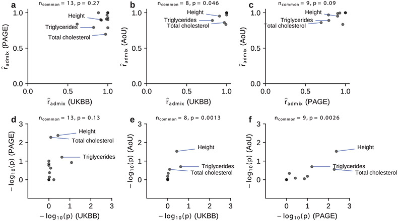
Extended Data Fig. 1 ∣. Consistency of ${\mathit{r}}_{\text{admix}}$ for shared traits across studies.

We compared estimated $r_{\text{admix}}$ for shared traits across studies. We compared both ${\widehat{r}}_{\text{admix}}$ (a–c) and $-{\log }_{10}(p)$ (for one-sided test of $H_0:r_{\text{admix}}=1$; Methods) (d-f). Three traits (Height, Triglycerides, Total cholesterol) with the most significant $p$-values for $H_0:r_{\text{admix}}=1$ were annotated. Number of common traits shared across studies $(n_{\text{common}})$ and Spearman correlation $p$-value were shown in the title for each panel. Overall, there were weak consistency of estimated ${\widehat{r}}_{\text{admix}}$ for shared traits across studies (although $p$-values for $H_0:r_{\text{admix}}=1$ were consistent significantly). Numerical results are reported in Supplementary Table 7.

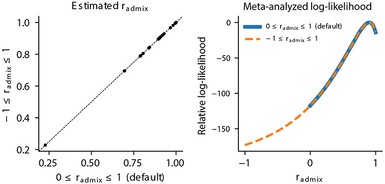
Extended Data Fig. 2 ∣. ${\mathit{r}}_{\mathbf{admix}}$ estimation is robust to the assumption of ${\mathit{r}}_{\mathbf{admix}}>0$.

We performed $r_{\text{admix}}$ estimation using alternative assumption of $-1\le r_{\text{admix}}\le 1$ in real trait analysis in PAGE in light of potential scenarios of effect sizes in opposite directions^36,63. We compared estimated $r_{\text{admix}}$ when assuming $0\le r_{\text{admix}}\le 1$ (default Methods) and when assuming $-1\le r_{\text{admix}}\le 1$. Left: comparing point estimates of $r_{\text{admix}}$ across 24 traits in PAGE. Right: comparing the meta-analyzed log-likelihood. Results obtained from two methods are highly consistent.

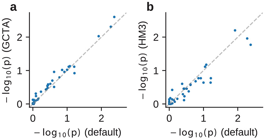
Extended Data Fig. 3 ∣. ${\mathit{r}}_{\mathbf{admix}}$ estimation is robust to genetic architecture and SNP set.

We performed $r_{\text{admix}}$ estimation under the assumption of alternative genetic architecture and SNP set on real trait analysis across PAGE and UKBB. We compared $p$-values (for one-sided test of $H_0:r_{\text{admix}}=1$) of our default setting (using frequency-dependent genetic architecture and imputed SNPs; Table 1) to those obtained using GCTA genetic architecture and imputed SNPs (a), and to those obtained using frequency-dependent genetic architecture and HM3 SNPs (b). Numerical results are reported in Supplementary Table 8.

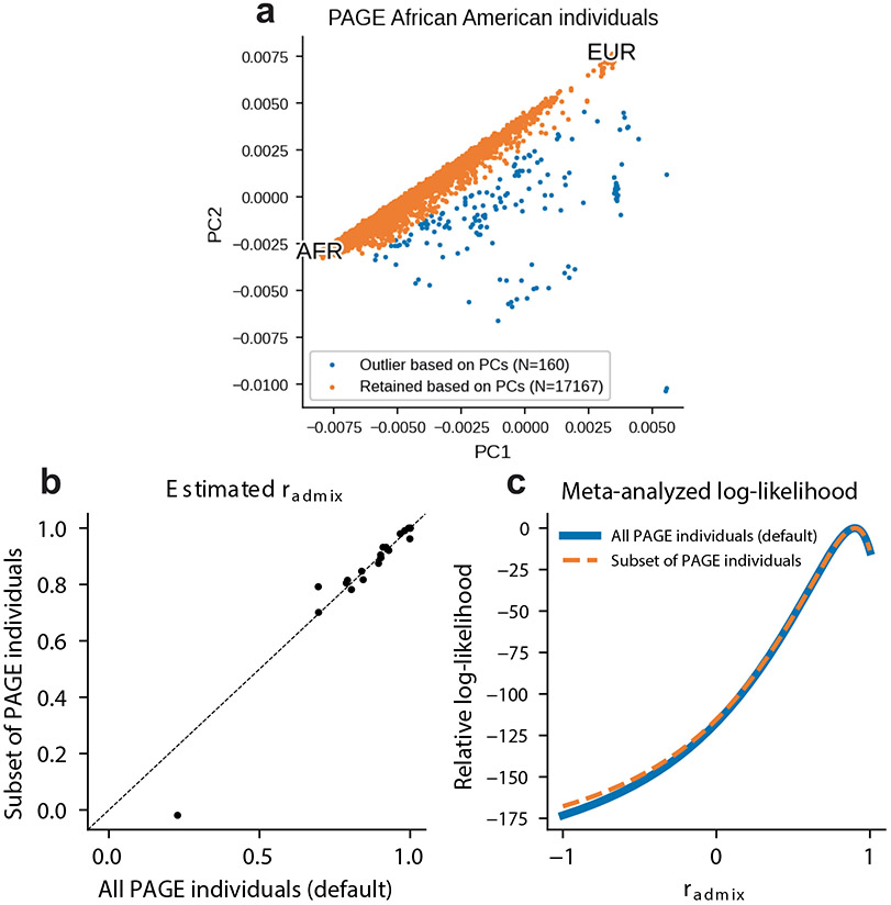
Extended Data Fig. 4 ∣. ${\mathit{r}}_{\mathbf{admix}}$ estimation is robust to subsetting PAGE African American individuals based on genotype PCs.

We subsetted PAGE individuals with self-identified race/ethnicity label of ‘African American’ (total N = 17,327) based on genotype PCs and retained N = 17,167 individuals (a). We found that the estimated $r_{\text{admix}}$ were highly consistent between using all PAGE African American individuals (default) and using subset of PAGE African American individuals based on genotype PCs. (b) comparing point estimates of $r_{\text{admix}}$ across 24 traits in PAGE. (Dot on the bottom left of the figure corresponds to MCHC trait, with a small sample size of 3,650.) (c) comparing the meta-analyzed log-likelihood. Results obtained from two sets of individuals are highly consistent.

Extended Data Fig. 5 ∣. Comparing estimated ${\mathit{r}}_{\mathbf{admix}}$ between alternative method formulations and default method.

Each dot corresponds to a trait. (a) Comparing results of default method and of directly optimizing and estimating ${\sigma }_g^2$, ${\rho }_g$. (b) Comparing results of default method and of directly optimizing and estimating ${\sigma }_{g,1}^2$, ${\sigma }_{g,2}^2$ (different variance components per ancestry) and ${\rho }_g$. See Supplementary Table 9 and Supplementary Note for details.

Extended Data Fig. 6 ∣. Multiple conditionally independent association signals for loci with heterogeneity by ancestry.

Upper panel corresponds to the two-sided association $p$-values and lower panel corresponds to the fine-mapping PIP. Different colors in the PIP plot corresponds to different credible sets. (a) MCH at 16p13.3 for UK Biobank European-African admixed individuals. (b) RBC at 16p13.3 for UK Biobank European-African admixed individuals. (c) CRP at 1q23.2 for PAGE European-African admixed individuals.

Extended Data Fig. 7 ∣. Simulations with single causal variant.

Simulations were based on 100 regions each spanning 20 Mb on chromosome 1 and 17,299 PAGE individuals. In each simulation, we randomly selected single causal variant and simulated quantitative phenotypes where these causal variants had same causal effects across ancestries and each causal variant was expected to explain a fixed amount of heritability (0.2%, 0.6%, 1.0%). Each panel corresponds to one metric for both causal and clumped variants. (a) False positive rate (FPR) of HET test. (b) Deming regression slope with ${\beta }_{\text{afr}}\sim {\beta }_{\text{eur}}$. (c) Deming regression slope with ${\beta }_{\text{eur}}\sim {\beta }_{\text{afr}}$. (d) Pearson correlation. (e) OLS regression slope with ${\beta }_{\text{afr}}\sim {\beta }_{\text{eur}}$. (f) OLS regression slope with ${\beta }_{\text{eur}}\sim {\beta }_{\text{afr}}$. 95% confidence intervals were based on 100 random sub-samplings with each sample consisted of 500 SNPs (Methods). Numerical results are reported in Supplementary Table 13.

Extended Data Fig. 8 ∣. Simulation with multiple causal variants at other sample sizes (Fig. 6d-f).

Simulations were based on chromosome 1 (515,087 SNPs) and 17,299 PAGE individuals. We drew 62,125, 250, 500, 1000 causal variants to simulate different level of polygenicity, such that on average there were approximately 0.25, 0.5, 1.0, 2.0, 4.0 causal variants per Mb. The heritability explained by all causal variants was fixed at $h_g^2=10\%$. (a-c) False positive rate of HET test for the causal variants and clumped variants. (d-f) Deming regression slope of estimated ancestry-specific effects $({\beta }_{\text{eur}}~{\beta }_{\text{af}})$ for the causal variants and clumped variants. 95% confidence intervals were based on 100 random sub-samplings with each sub-sample consisted of $n=50,100,500$ SNPs (instead of n = 1,000 SNPs in Fig. 6c, d) (Methods).

Extended Data Fig. 9 ∣. Additional results for simulations with single causal variant with varying ${\beta }_{\mathbf{eur}}:{\beta }_{\mathbf{afr}}$ and $h_g^2$.

Simulations were based on 100 regions each spanning 20 Mb on chromosome 1 from 17299 PAGE individuals. In each simulation, we randomly selected single causal variant and simulated quantitative phenotypes where these causal variants had varying causal effects across ancestries and each causal variant was expected to explain a fixed amount of heritability (0.2%, 0.6%, 1.0%, 2.0%, 5.0%). We provide results for both causal variants and LD-clumped variants. We separate results into two rows for better visualization: upper row (a-c): ${\beta }_{\text{eur}}:{\beta }_{\text{afr}}=0.9,1.0,1.1$; lower row (d-f): ${\beta }_{\text{eur}}:{\beta }_{\text{afr}}=0.0$. We show results for False positive rate (FPR) of HET test, Deming regression slope with ${\beta }_{\text{eur}}~{\beta }_{\text{afr}}$, and OLS regression slope with ${\beta }_{\text{eur}}~{\beta }_{\text{afr}}$. 95% confidence intervals were based on 100 random sub-samplings with each sample consisted of 500 SNPs (Methods). Numerical results and further discussions are provided in Supplementary Table 15.

Data availability

PAGE individual-level genotype and phenotype data are available through dbGaP https://www.ncbi.nlm.nih.gov/projects/gap/cgi-bin/study.cgi?study_id=phs000356.v2.p1. UKBB individual-level genotype and phenotype data are available through application at https://www.ukbiobank.ac.uk/. AoU individual-level genotype and phenotype are available through application at https://www.researchallofus.org/. The set of preprocessed HapMap3 variants used in this manuscript is retrieved from https://ndownloader.figshare.com/files/25503788.

Code availability

Software implementing genome-wide genetic correlation estimation method: https://github.com/kangchenghou/admix-kit (ref. https://doi.org/10.5281/ZENODO.7482679) Code for replicating analyses: https://github.com/kangchenghou/admix-genet-cor (ref. https://doi.org/10.5281/ZENODO.7482683).

References

- 1.Wojcik GL et al. Genetic analyses of diverse populations improves discovery for complex traits. Nature 570, 514–518 (2019). [DOI] [PMC free article] [PubMed] [Google Scholar]
- 2.Bycroft C. et al. The UK Biobank resource with deep phenotyping and genomic data. Nature 562, 203–209 (2018). [DOI] [PMC free article] [PubMed] [Google Scholar]
- 3.Ramirez AH et al. The All of Us Research Program: data quality, utility, and diversity. Patterns 3, 100570 (2022). [DOI] [PMC free article] [PubMed] [Google Scholar]
- 4.Zhou W. et al. Global Biobank Meta-analysis Initiative: Powering genetic discovery across human disease. Cell Genomics 2, 100192 (2022). [DOI] [PMC free article] [PubMed] [Google Scholar]
- 5.Brown BC, Ye CJ, Price AL & Zaitlen N Transethnic genetic-correlation estimates from summary statistics. Am. J. Hum. Genet 99, 76–88 (2016). [DOI] [PMC free article] [PubMed] [Google Scholar]
- 6.Galinsky KJ et al. Estimating cross-population genetic correlations of causal effect sizes. Genet. Epidemiol 43, 180–188 (2019). [DOI] [PMC free article] [PubMed] [Google Scholar]
- 7.Shi H. et al. Localizing components of shared transethnic genetic architecture of complex traits from GWAS summary data. Am. J. Hum. Genet 106, 805–817 (2020). [DOI] [PMC free article] [PubMed] [Google Scholar]
- 8.Shi H. et al. Population-specific causal disease effect sizes in functionally important regions impacted by selection. Nat. Commun 12, 1098 (2021). [DOI] [PMC free article] [PubMed] [Google Scholar]
- 9.Kanai M. et al. Insights from complex trait fine-mapping across diverse populations. Preprint at medRxiv 10.1101/2021.09.03.21262975 (2021). [DOI] [Google Scholar]
- 10.Wang Y et al. Theoretical and empirical quantification of the accuracy of polygenic scores in ancestry divergent populations. Nat. Commun 11, 3865 (2020). [DOI] [PMC free article] [PubMed] [Google Scholar]
- 11.Martin AR et al. Clinical use of current polygenic risk scores may exacerbate health disparities. Nat. Genet 51, 584–591 (2019). [DOI] [PMC free article] [PubMed] [Google Scholar]
- 12.Gurdasani D, Barroso I, Zeggini E & Sandhu MS Genomics of disease risk in globally diverse populations. Nat. Rev. Genet 20, 520–535 (2019). [DOI] [PubMed] [Google Scholar]
- 13.Sirugo G, Williams SM & Tishkoff SA The missing diversity in human genetic studies. Cell 177, 1080 (2019). [DOI] [PMC free article] [PubMed] [Google Scholar]
- 14.Marigorta UM & Navarro A High trans-ethnic replicability of GWAS results implies common causal variants. PLoS Genet. 9, e1003566 (2013). [DOI] [PMC free article] [PubMed] [Google Scholar]
- 15.Patel RA et al. Genetic interactions drive heterogeneity in causal variant effect sizes for gene expression and complex traits. Am. J. Hum. Genet 109, 1286–1297 (2022). [DOI] [PMC free article] [PubMed] [Google Scholar]
- 16.Cai N et al. Minimal phenotyping yields genome-wide association signals of low specificity for major depression. Nat. Genet 52, 437–447 (2020). [DOI] [PMC free article] [PubMed] [Google Scholar]
- 17.Seldin MF, Pasaniuc B & Price AL New approaches to disease mapping in admixed populations. Nat. Rev. Genet 12, 523–528 (2011). [DOI] [PMC free article] [PubMed] [Google Scholar]
- 18.Mills MC & Rahal C The GWAS Diversity Monitor tracks diversity by disease in real time. Nat. Genet 52, 242–243 (2020). [DOI] [PubMed] [Google Scholar]
- 19.Atkinson EG et al. Tractor uses local ancestry to enable the inclusion of admixed individuals in GWAS and to boost power. Nat. Genet 53, 195–204 (2021). [DOI] [PMC free article] [PubMed] [Google Scholar]
- 20.Hou K, Bhattacharya A, Mester R, Burch KS & Pasaniuc B On powerful GWAS in admixed populations. Nat. Genet 53, 1631–1633 (2021). [DOI] [PMC free article] [PubMed] [Google Scholar]
- 21.Bitarello BD & Mathieson I Polygenic scores for height in admixed populations. G3 10, 4027–4036 (2020). [DOI] [PMC free article] [PubMed] [Google Scholar]
- 22.Marnetto D et al. Ancestry deconvolution and partial polygenic score can improve susceptibility predictions in recently admixed individuals. Nat. Commun 11, 1628 (2020). [DOI] [PMC free article] [PubMed] [Google Scholar]
- 23.Bentley AR et al. Gene-based sequencing identifies lipid-influencing variants with ethnicity-specific effects in African Americans. PLoS Genet. 10, e1004190 (2014). [DOI] [PMC free article] [PubMed] [Google Scholar]
- 24.Rajabli F et al. Ancestral origin of ApoE ε4 Alzheimer disease risk in Puerto Rican and African American populations. PLoS Genet. 14, e1007791 (2018). [DOI] [PMC free article] [PubMed] [Google Scholar]
- 25.Blue EE, Horimoto ARVR, Mukherjee S, Wijsman EM & Thornton TA Local ancestry at APOE modifies Alzheimer’s disease risk in Caribbean Hispanics. Alzheimers Dement. 15, 1524–1532 (2019). [DOI] [PMC free article] [PubMed] [Google Scholar]
- 26.Naslavsky MS et al. Global and local ancestry modulate APOE association with Alzheimer’s neuropathology and cognitive outcomes in an admixed sample. Mol. Psychiatry 27, 4800–4808 (2022). [DOI] [PMC free article] [PubMed] [Google Scholar]
- 27.Yang J, Lee SH, Goddard ME & Visscher PM GCTA: a tool for genome-wide complex trait analysis. Am. J. Hum. Genet 88, 76–82 (2011). [DOI] [PMC free article] [PubMed] [Google Scholar]
- 28.Sakaue S et al. A cross-population atlas of genetic associations for 220 human phenotypes. Nat. Genet 53, 1415–1424 (2021). [DOI] [PubMed] [Google Scholar]
- 29.Zeng J et al. Signatures of negative selection in the genetic architecture of human complex traits. Nat. Genet 50, 746–753 (2018). [DOI] [PubMed] [Google Scholar]
- 30.Schoech AP et al. Quantification of frequency-dependent genetic architectures in 25 UK Biobank traits reveals action of negative selection. Nat. Commun 10, 790 (2019). [DOI] [PMC free article] [PubMed] [Google Scholar]
- 31.Zhang Y, Qi G, Park J-H & Chatterjee N Estimation of complex effect-size distributions using summary-level statistics from genome-wide association studies across 32 complex traits. Nat. Genet 50, 1318–1326 (2018). [DOI] [PubMed] [Google Scholar]
- 32.The International HapMap 3 Consortium. Integrating common and rare genetic variation in diverse human populations. Nature 467, 52–58 (2010). [DOI] [PMC free article] [PubMed] [Google Scholar]
- 33.Speed D & Balding DJ SumHer better estimates the SNP heritability of complex traits from summary statistics. Nat. Genet 51, 277–284 (2019). [DOI] [PMC free article] [PubMed] [Google Scholar]
- 34.Deming WE Statistical adjustment of data. Wiley. (1943). [Google Scholar]
- 35.Pasaniuc B. et al. Enhanced statistical tests for GWAS in admixed populations: assessment using African Americans from CARe and a Breast Cancer Consortium. PLoS Genet. 7, e1001371 (2011). [DOI] [PMC free article] [PubMed] [Google Scholar]
- 36.Hodonsky CJ et al. Ancestry-specific associations identified in genome-wide combined-phenotype study of red blood cell traits emphasize benefits of diversity in genomics. BMC Genomics 21, 228 (2020). [DOI] [PMC free article] [PubMed] [Google Scholar]
- 37.Loh P-R et al. Contrasting genetic architectures of schizophrenia and other complex diseases using fast variance-components analysis. Nat. Genet 47, 1385–1392 (2015). [DOI] [PMC free article] [PubMed] [Google Scholar]
- 38.Johnson R et al. Estimation of regional polygenicity from GWAS provides insights into the genetic architecture of complex traits. PLoS Comput. Biol 17, e1009483 (2021). [DOI] [PMC free article] [PubMed] [Google Scholar]
- 39.Zhang J & Stram DO The role of local ancestry adjustment in association studies using admixed populations. Genet. Epidemiol 38, 502–515 (2014). [DOI] [PMC free article] [PubMed] [Google Scholar]
- 40.Liu J, Lewinger JP, Gilliland FD, Gauderman WJ & Conti DV Confounding and heterogeneity in genetic association studies with admixed populations. Am. J. Epidemiol 177, 351–360 (2013). [DOI] [PMC free article] [PubMed] [Google Scholar]
- 41.Saitou M, Dahl A, Wang Q & Liu X Allele frequency differences of causal variants have a major impact on low cross-ancestry portability of PRS. Preprint at medRxiv 10.1101/2022.10.21.22281371 (2022). [DOI] [Google Scholar]
- 42.Pasaniuc B et al. Analysis of Latino populations from GALA and MEC studies reveals genomic loci with biased local ancestry estimation. Bioinformatics 29, 1407–1415 (2013). [DOI] [PMC free article] [PubMed] [Google Scholar]
- 43.Yang J et al. Common SNPs explain a large proportion of the heritability for human height. Nat. Genet 42, 565–569 (2010). [DOI] [PMC free article] [PubMed] [Google Scholar]
- 44.Speed D, Hemani G, Johnson MR & Balding DJ Improved heritability estimation from genome-wide SNPs. Am. J. Hum. Genet 91, 1011–1021 (2012). [DOI] [PMC free article] [PubMed] [Google Scholar]
- 45.Gazal S et al. Linkage disequilibrium-dependent architecture of human complex traits shows action of negative selection. Nat. Genet 49, 1421–1427 (2017). [DOI] [PMC free article] [PubMed] [Google Scholar]
- 46.Gazal S, Marquez-Luna C, Finucane HK & Price AL Reconciling S-LDSC and LDAK functional enrichment estimates. Nat. Genet 51, 1202–1204 (2019). [DOI] [PMC free article] [PubMed] [Google Scholar]
- 47.Hou K et al. Accurate estimation of SNP-heritability from biobank-scale data irrespective of genetic architecture. Nat. Genet 51, 1244–1251 (2019). [DOI] [PMC free article] [PubMed] [Google Scholar]
- 48.Linnet K Performance of Deming regression analysis in case of misspecified analytical error ratio in method comparison studies. Clin. Chem 44, 1024–1031 (1998). [PubMed] [Google Scholar]
- 49.Chiu AM, Molloy EK, Tan Z, Talwalkar A & Sankararaman S Inferring population structure in biobank-scale genomic data. Am. J. Hum. Genet 109, 727–737 (2022). [DOI] [PMC free article] [PubMed] [Google Scholar]
- 50.Chang CC et al. Second-generation PUNK: rising to the challenge of larger and richer datasets. Gigascience 4, 7 (2015). [DOI] [PMC free article] [PubMed] [Google Scholar]
- 51.Loh P-R et al. Reference-based phasing using the Haplotype Reference Consortium panel. Nat. Genet 48, 1443–1448 (2016). [DOI] [PMC free article] [PubMed] [Google Scholar]
- 52.Maples BK, Gravel S, Kenny EE & Bustamante CD RFMix: a discriminative modeling approach for rapid and robust local-ancestry inference. Am. J. Hum. Genet 93, 278–288 (2013). [DOI] [PMC free article] [PubMed] [Google Scholar]
- 53.The 1000 Genomes Project Consortium, et al. A global reference for human genetic variation. Nature 526, 68–74 (2015). [DOI] [PMC free article] [PubMed] [Google Scholar]
- 54.Schubert R, Andaleon A & Wheeler HE Comparing local ancestry inference models in populations of two- and three-way admixture. Peer J 8, e10090 (2020). [DOI] [PMC free article] [PubMed] [Google Scholar]
- 55.Gay NR et al. Impact of admixture and ancestry on eQTL analysis and GWAS colocalization in GTEx. Genome Biol. 21, 233 (2020). [DOI] [PMC free article] [PubMed] [Google Scholar]
- 56.Pardiñas AF et al. Common schizophrenia alleles are enriched in mutation-intolerant genes and in regions under strong background selection. Nat. Genet 50, 381–389 (2018). [DOI] [PMC free article] [PubMed] [Google Scholar]
- 57.Schoech AP et al. Negative short-range genomic autocorrelation of causal effects on human complex traits. Preprint at medRxiv 10.1101/2020.09.23.310748 (2020). [DOI] [Google Scholar]
- 58.Bulik-Sullivan B et al. An atlas of genetic correlations across human diseases and traits. Nat. Genet 47, 1236–1241 (2015). [DOI] [PMC free article] [PubMed] [Google Scholar]
- 59.Reich D et al. Reduced neutrophil count in people of African descent is due to a regulatory variant in the Duffy antigen receptor for chemokines gene. PLoS Genet. 5, e1000360 (2009). [DOI] [PMC free article] [PubMed] [Google Scholar]
- 60.Reiner AP et al. Genome-wide association and population genetic analysis of C-reactive protein in African American and Hispanic American women. Am. J. Hum. Genet 91, 502–512 (2012). [DOI] [PMC free article] [PubMed] [Google Scholar]
- 61.Manichaikul A et al. Robust relationship inference in genome-wide association studies. Bioinformatics 26, 2867–2873 (2010). [DOI] [PMC free article] [PubMed] [Google Scholar]
- 62.Wang G, Sarkar A, Carbonetto P & Stephens M A simple new approach to variable selection in regression, with application to genetic fine mapping. J. R. Stat. Soc. Ser. B 82, 1273–1300 (2020). [DOI] [PMC free article] [PubMed] [Google Scholar]
- 63.Cook JP & Morris AP Multi-ethnic genome-wide association study identifies novel locus for type 2 diabetes susceptibility. Eur. J. Hum. Genet 24, 1175–1180 (2016). [DOI] [PMC free article] [PubMed] [Google Scholar]
Associated Data
This section collects any data citations, data availability statements, or supplementary materials included in this article.
Supplementary Materials
Data Availability Statement