Relationship between protein folding thermodynamics and the energy landscape

Abstract

The origin of protein folding thermodynamics is examined in terms of the energy landscape, employing an off-lattice protein model with scaled non-native attractions, which is continuously tunable between a Go-like model and a highly frustrated system. Extensive statistical temperature molecular dynamics simulations, combined with inherent structure analysis, reveal the intimate connection between the global geometric properties of the energy landscape and the statistical temperature. The basin depth of the energy landscape is shown to play a key role in the first-order-like characteristics of the statistical temperature, which are easily identified by the squared modulus of the potential energy gradient in the microcanonical ensemble.

Protein folding—i.e., how a polypeptide chain reaches a unique native state for a given sequence of amino acids [1]—is one of the fundamental problems in biological science. While significant advances have been made [2–9], fundamental open questions still remain. For example, one would like to understand the remarkable observation that most single-domain proteins exhibit a cooperative, two-state folding transition with no detectable intermediates [2].

Energy landscape theory [3–6] provides a theoretical framework for protein folding, in which the connection between a proteinlike sequence and a minimally frustrated energy landscape is rationalized via a folding funnel [4]. A good folding sequence is characterized by a smooth potential energy landscape (PEL), with an overall funnel shape biased to the native state, while a poorly designed sequence like a random heteropolymer has a rugged PEL susceptible to long-lived kinetic trapping [7]. Many simulation studies have been devoted to elucidate the determinants of a proteinlike system, such as the ratio of the folding and glass transition temperatures [3], the stability gap between a native state and low-lying excited states [8], and the collapse cooperativity [9].

Recently, Mazzoni and Casetti [10] proposed the fluctuations of the energy landscape curvature, $K_R={\nabla }^{2}U,U$ being the potential energy, as a determinant. A dramatic enhancement of the fluctuations, $\kappa \left(T\right)=\sqrt{\left(⟨K_R^2⟩-{⟨K_R⟩}^2\right)}/⟨K_R⟩$, in the vicinity of the folding temperature $T=T_f$ was observed in the proteinlike folding of well-designed sequences, where ⟨⋅⟩ denotes an equilibrium average. The enhancement in $\kappa \left(T_f\right)$ is attributed to effective two-state dynamics between the native and denatured states with different curvatures [10].

Two-state protein folding is analogous to a first-order phase transition in finite-size systems [11–13]. Indeed, a recent study [14] reveals that the “backbending” ($S$ bend) in the statistical temperature, or microcanonical caloric curve, characteristic of a first-order-like phase transition, fully characterizes protein folding and clearly distinguishes good folders from poor ones. The question naturally arises: how does the global geometry of the PEL translate into the behavior of the statistical temperature? This paper addresses the issue by establishing a rigorous connection between the statistical temperature and various energy landscape measures, leading to the identification of the principal landscape determinants of two-state folding thermodynamics.

The key quantity in our study is the statistical temperature in the microcanonical ensemble, $T_S\left(U\right)=[\partial S(U)/\partial U{]}^{-1},S(U)$ being the microcanonical entropy. It is well known that in a finite-size system such as a protein, the microcanonical ensemble is well suited to the analysis of phase transitions [11–14]. Around a first-order phase transition, $S\left(U\right)$ shows a convex dip, with ${\partial }^{2}S/\partial U^2>0$, corresponding to backbending in $T_S\left(U\right)$ or a negative specific heat. Backbending is associated with an extremum condition in the Helemholtz free energy at $T_f,F\left(U,T_f\right)=U-T_{f}S\left(U\right)$, which has three roots $U_i(i=1-3)$, satisfying $T_S\left(U_i\right)=T_f\left(U_1<U_2<U_3\right)$. The multiple roots are associated with two-state transition behavior between free-energy minima at $U_1$ and $U_3$, involving the crossing of a transition barrier at $U_2$, while the transition becomes downhill-like without a barrier for the monotonic $T_S\left(U\right)$ Thus, all essential features of the transitions occurring in good and poor folders are completely characterized by the behavior of $T_S\left(U\right)$.

Our analysis linking $T_S\left(U\right)$ to the PEL is based on the thermodynamic identity between the statistical temperature and the configurational temperature $T_{\mathit{\text{conF}}}\left(U\right)$ originally introduced by Rugh [15] and later generalized by Jepps et al. [16]:

$$T_S\left(U\right)=T_{\mathit{\text{conF}}}\left(U\right)=\frac{{⟨\parallel \nabla U{\parallel }^2⟩}_U}{{⟨{\nabla }^{2}U⟩}_U}=\frac{ℱ\left(U\right)}{𝒦\left(U\right)},$$ (1)

where the subscript “$\mathrm{c}\mathrm{o}\mathrm{n}F$” implies that the configurational temperature is evaluated as the fraction of two separate microcanonical averages, $ℱ\left(U\right)={⟨\parallel \nabla U{\parallel }^2⟩}_U$ and $𝒦\left(U\right)={⟨{\nabla }^{2}U⟩}_U$ [16]. The significance of Eq. (1) is that it allows a rigorous mathematical connection between the purely statistical quantity $T_S\left(U\right)$ and the geometric structure of the energy landscape via the force, $\mathbf{F}=-\nabla U$, and the curvature, $K_R={\nabla }^{2}U$.

All-atom simulations considering the protein and explicit solvent are the most accurate, but still computationally demanding. Thus a simplified description, retaining the main features of real proteins, but reducing the number of degrees of freedom through a coarse graining, is especially appealing for the characterization of protein-folding mechanisms over long time scales. The newly suggested folding determinants [10,14] have been examined in coarse-grained models, with varied sequences exhibiting a different foldability.

Here we employ the scaled Honeycutt-Thirumalai (SHT) off-lattice model [17] to mimic the effect of sequence variations and to examine how two-state folding results from the global shape of the PEL and the emerging backbending behavior of $T_S\left(U\right)$. The original HT model [18] has a $\beta$-barrel native state and consists of 46 beads with three different types: hydrophobic $\left(B\right)$, hydrophilc $\left(L\right)$, and neutral $\left(N\right)$. We modified the model to incorporate scaled, Go-like interactions by modulating the attractions between non-native $BB$ contacts, which allows, for the original HT sequence $B_9{N}_3\left(LB{)}_4{N}_3{B}_9{N}_3\right(LB{)}_{5}L$, a continuous tuning from a highly frustrated PEL to a weakly rugged funnel. The potential energy is a sum of bond stretching $\left(U_B\right)$, bending $\left(U_A\right)$, torsion $\left(U_T\right.$), and nonbonded interactions ($U_{NB,\lambda }$):

$$U\left(\mathbf{r};\lambda \right)=U_B+U_A+U_T+U_{NB,\lambda },$$ (2)

where $U_B={\Sigma }_i{k}_r{\left(r_i-r_e\right)}^2,U_A={\Sigma }_i{k}_{\theta }{\left({\theta }_i-{\theta }_e\right)}^2$, and $U_T={\Sigma }_i\left\{A_i[1\right.\left.\left.+\mathrm{c}\mathrm{o}\mathrm{s}\left({\varphi }_i\right)\right]+B_i\left[1+\mathrm{c}\mathrm{o}\mathrm{s}\left(3{\varphi }_i\right)\right]\right\}$. The stretching and bending constants are $k_r=200ϵ/{\sigma }^2$ and $k_{\theta }=10ϵ/{\mathrm{r}\mathrm{a}\mathrm{d}}^2$, respectively, $ϵ$ and $\sigma$ being energy and length units, with $r_e=\sigma$ and ${\theta }_e={105}^{\circ }$. Torsion parameters are $A_i=B_i=1.2$ for a quartet of successive beads with zero or one $N$ bead, while otherwise $A_i=0$ and $B_i=0.2$.

The nonbonded term in Eq. (2) contains the scaling factor $\lambda (0⩽\lambda ⩽1)$ to modulate the non-native attractions as $U_{NB,\lambda }={\Sigma }_{i<j-3}\left[U_{ij}+(\lambda -1)U_{ij}\delta (i,\alpha )\delta (j,\alpha )\right],U_{ij}=4ϵS_1\left[{\left(\sigma /r_{ij}\right)}^{12}-S_2{\left(\sigma /r_{ij}\right)}^6\right]$, where $S_1=S_2=1$ for $BB$ pairs, $S_1=2/3$ and $S_2=-1$ for $LL$ and $LB$ pairs, and $S_1=1$ and $S_2=0$ for all other pairs involving $N$. Here $\delta (i,\alpha )=1$ if $\alpha =B$ and bead $i$ belongs to the non-native contact set, and otherwise $\delta (i,\alpha )=0$. As $\lambda$ approaches zero, the second term in $U_{NB,\lambda }$ introduces a strong native bias in denatured states by prohibiting close contacts between non-native $BB$ pairs. All 57 native contact pairs are identified with the cutoff $1.3\sigma$, based on the global minimum structure of the original HT model $(U=-49.2635)$.

Due to the high degree of frustration in the original HT model [18,19], an enhanced sampling technique is indispensable to obtain a correct conformational sampling for both the transition and low-temperature regions, overcoming ergodicity breaking. We applied the statistical temperature molecular dynamics (STMD) algorithm [19], which generates a flat energy sampling via the dynamic refinement of the statistical temperature (for details see Ref. [19]) with four different scalings at $\lambda =1.0,0.9,0.5$, and 0. All STMD simulations have been performed to sample the temperature range from 0.07 to 1.3, with the average kinetic energy fixed at $T_0=1.3$. A total of 8 × 10⁴ configurations for each simulation were collected to determine the canonical and microcanonical thermodynamics, and minimized using the conjugate-gradient algorithm to map inherent structures (ISs) [20].

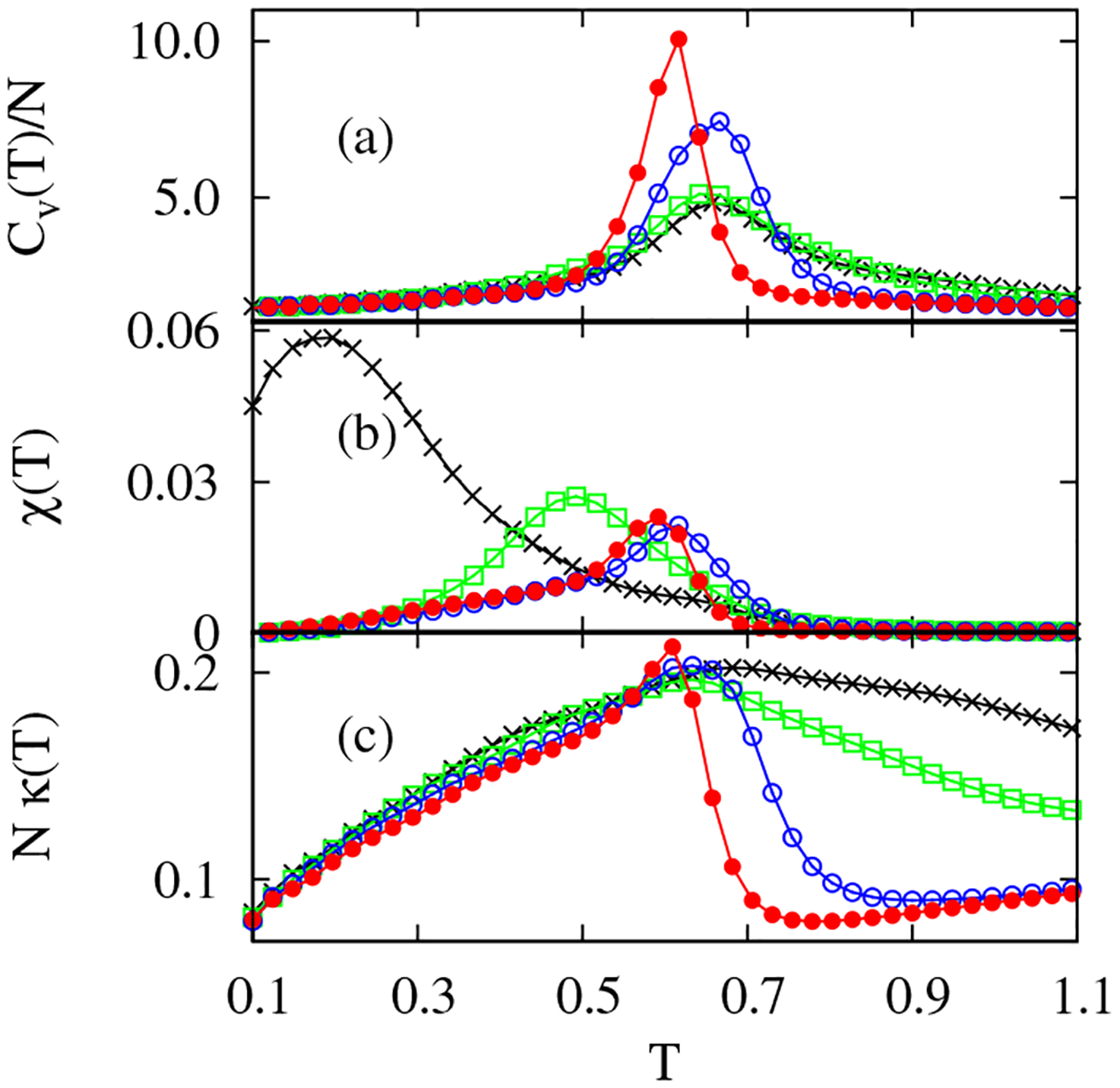
As summarized in Table I, the folding $\left(T_f\right)$ and collapse $\left(T_{\theta }\right)$ temperatures, identified by peaks in the $T$-dependent heat capacities and order parameter fluctuations in Figs. 1(a) and 1(b), respectively, illustrate that the original HT model (SHT with $\lambda =1$) is a poor folder and the SHT model with $\lambda =0.9$ is an intermediate folder, while $\lambda =0.5$ and 0 correspond to good folders according to the classification based on the collapse cooperativity, $\sigma =\left(T_{\theta }-T_f\right)/T_{\theta }$ [9]. The validity of this classification is also seen in the profiles of the curvature fluctuations $\kappa \left(T\right)$ in Fig. 1(c). A marked peak shows up close to $T_f$ for good folders, while the plots are featureless in poor and intermediate folders [10]. Note that the temperature $T_{\kappa }$, corresponding to the maximum curvature fluctuation in Fig. 1(c), coincides with $T_f$ for good folders, implying that $\kappa \left(T\right)$ is also an effective folding indicator.

TABLE I.

Characteristic temperatures of folding $\left(T_f\right)$, collapse $\left(T_{\theta }\right)$, and curvature fluctuation $\left(T_{\kappa }\right)$ and the collapse cooperativity $\sigma$ at different $\lambda =1.0,0.9,0.5$, and 0.

Scaling parameter $\mathit{\lambda }$	${\mathit{T}}_{\mathit{f}}$	${\mathit{T}}_{\mathit{\theta }}$	${\mathit{T}}_{\mathit{\kappa }}$	$\mathit{\sigma }=\left({\mathit{T}}_{\mathit{\theta }}-{\mathit{T}}_{\mathit{f}}\right)/{\mathit{T}}_{\mathit{\theta }}$
1.0	0.19	0.67	0.68	0.71
0.9	0.49	0.65	0.64	0.25
0.5	0.61	0.67	0.62	0.09
0.0	0.59	0.62	0.60	0.05

FIG. 1.

(Color online) (a) Specific heats $C_v\left(T\right)$, (b) order parameter fluctuations $\chi \left(T\right)$, and (c) curvature fluctuations $\kappa \left(T\right)$ at different $\lambda =1.0,0.9,0.5$, and 0 from bottom to top in (a) at $T=0.6$.

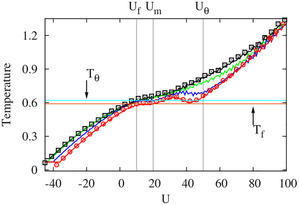
The statistical temperature $T_S\left(U\right)$, determined by STMD in Fig. 2, shows a dramatic change as the energy landscape changes with decreasing $\lambda$. The smooth, monotonically varying $T_S\left(U\right)$ in the original HT model $(\lambda =1)$ first starts to show a plateau, or weak backbending, and a substantial backbending appears as $\lambda$ falls below 0.5. Remarkably, the temperatures corresponding to the plateau and backbending regions in $T_S\left(U\right)$ with $\lambda =0$ exactly match $T_f$ and $T_{\theta }$, respectively. The alteration of the folding mechanism from second-order-like collapse $(\lambda =1)$ into first-order-like folding $(\lambda =0)$ is clearly seen through the behavior of $T_S\left(U\right)$.

FIG. 2.

(Color online) Statistical temperatures $T_S\left(U\right)$ (solid lines) and configurational temperatures $T_{\mathit{\text{conF}}}\left(U\right)$ (squares and circles) with different $\lambda =1.0,0.9,0.5$, and 0 from top to bottom at $U=40$. Note that horizontal lines at $T_{\theta }=0.62$ and $T_f=0.59$ match the backbending and plateau regions of $T_S\left(U\right)$ at $\lambda =0$, respectively.

We find that the folding in Go-like models occurs through the transient formation of a three-strand core near $T_{\theta }$ and the immediate attachment of the terminal strand to attain the native state at $T_f\left(\simeq T_{\theta }\right)$. A significant slowing down is observed in the folding of the original HT model with $T_f\ll T_{\theta }$ due to trapping in misfolded states. Since $U$ is the external control parameter in the microcanonical ensemble (playing the role of the temperature in the canonical ensemble), we also identify the characteristic energies to describe the folding transition as a function of $U$, in the case of $\lambda =0$. In Fig. 2, both $U_f=10$ and $U_m=20$ approximately define the plateau region in $T_S\left(U\right)$, and both $U_m$ and $U_{\theta }=50$ bound the collapse region associated with the backbending of $T_S\left(U\right)$, $T_S\left(U_{\theta }\right)=0.65$. The good folder with $\lambda =0$ starts to collapse as $U$ crosses $U_{\theta }$, and completes its folding once $U$ passes through $U_f$.

Assuming that STMD samples all configurations with a given $U$, the microcanonical average in Eq. (1) is directly computed by binning in energy and collecting configurations corresponding to each bin. The configurational temperature $T_{\mathit{\text{conF}}}\left(U\right)$ with unit bin size shows good agreement with $T_S\left(U\right)$ in both $\lambda =1$ and 0, illustrating that the thermodynamic identity, Eq. (1), is robust even with a smaller system size.

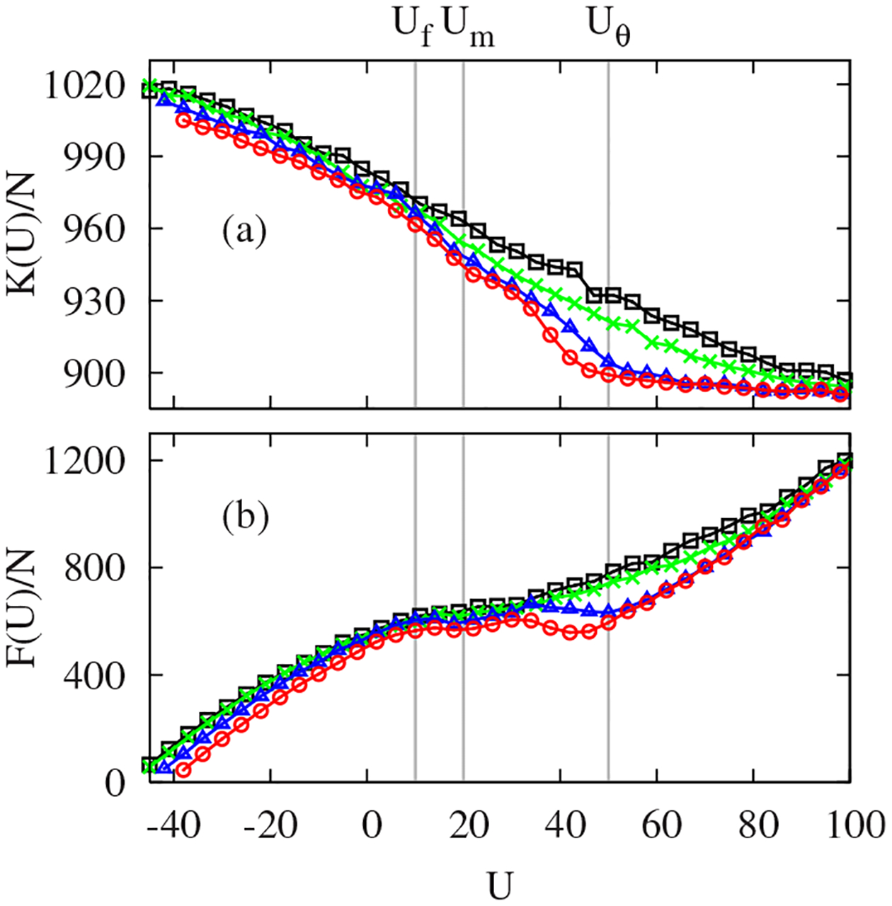
To illustrate how the PEL controls $T_S\left(U\right)$, and hence the folding, via Eq. (1), both $𝒦\left(U\right)$ and $ℱ\left(U\right)$ are plotted in Figs. 3(a) and 3(b), respectively. For all scalings, the curvature $𝒦\left(U\right)$ monotonically increases with decreasing $U$, showing that folded (denatured) states are associated with steeper (shallow) potential wells. The primary feature differentiating good from poor folders in Fig. 3(a) is that good folders have nearly constant curvature for $U>U_{\theta }$, suggesting that their denatured states are structurally homogeneous. This finding is in accordance with our expectations for Go-like interactions. The main frustration of the original HT model arises from the conformational diversity of the collapsed states [18]. The native-centric $U_{NB,\lambda }$ in Go-like models significantly suppresses the frustration from hydrophobic mismatches of $\beta$ strands during the collapse by reducing non-native interstrand $BB$ contacts and also makes the unfolded landscape less structured. With decreasing $U$ in good folders, the flat $𝒦\left(U\right)$ begins to increase steeply between $U_f$ and $U_{\theta }$, the backbending and plateau regions of $T_S\left(U\right)$, contributing to the large curvature fluctuation $\kappa \left(T_f\right)$ and to the bimodal energy distributions [10]. By contrast, in poor folders the slope of $𝒦\left(U\right)$ is nearly constant, causing no structure in $T_S\left(U\right)$ and corresponding to the fact that all systems studied have nearly identical $𝒦\left(U\right)$ at the highest and lowest $U$.

FIG. 3.

(Color online) Microcanonical average of (a) $𝒦\left(U\right)$ and (b) $ℱ\left(U\right)$ with different $\lambda =1.0,0.9,0.5$, and 0 from top to bottom around $U=40$.

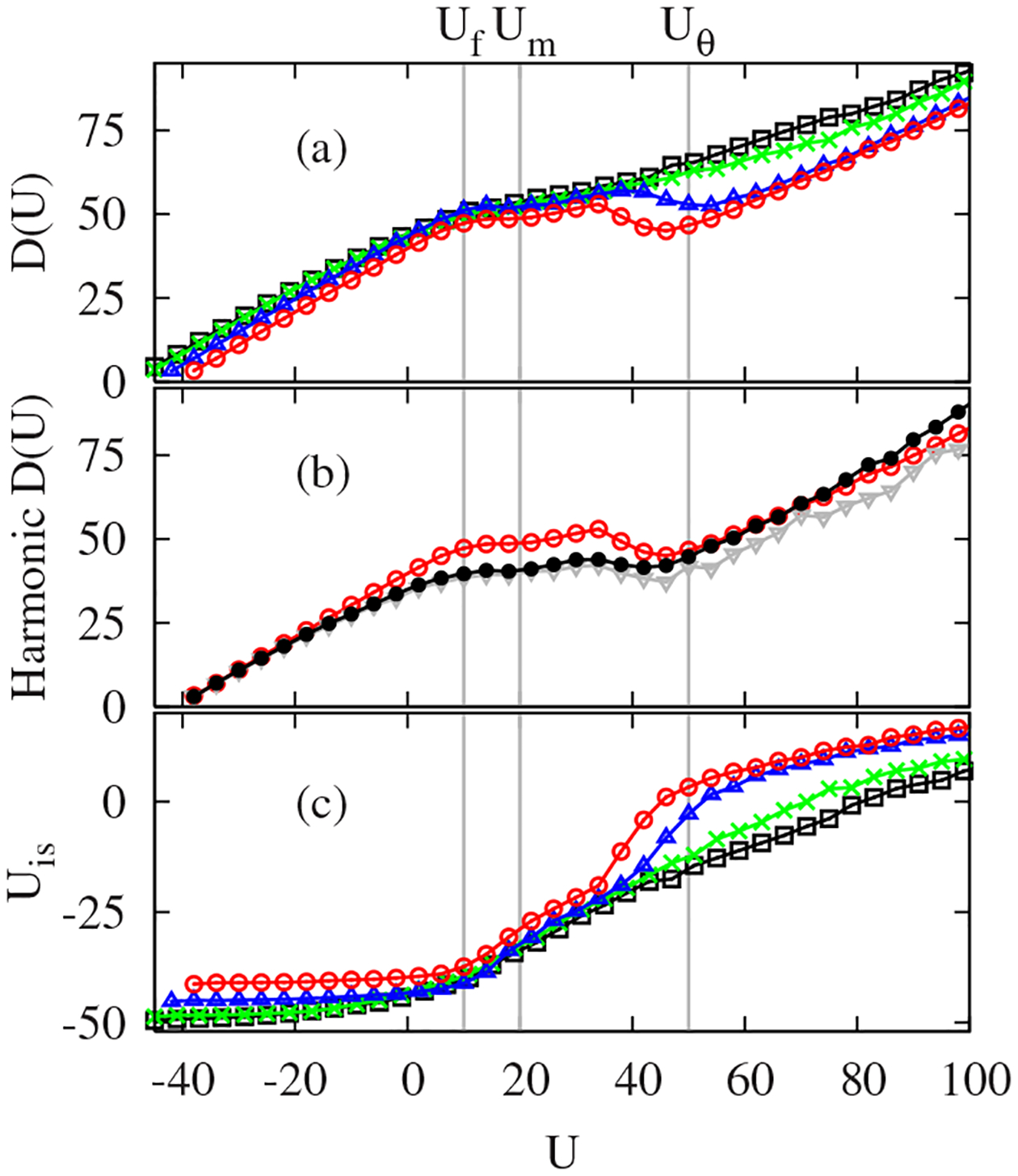
Turning to $ℱ\left(U\right)$, the most remarkable aspect of Fig. 3(b) is that $ℱ\left(U\right)$ retains all essential features of $T_S\left(U\right)$. Despite the discussion in the last paragraph, the dynamic range of $𝒦\left(U\right)$ is small and the variation of $T_S\left(U\right)$ is mostly encoded into $ℱ\left(U\right)$. What is the underlying physics relating $ℱ\left(U\right)$ to $T_S\left(U\right)$? Some insight is gained by noting that $ℱ\left(U\right)$ is a measure of the geometric distance between the sampled configurations at $U$ and their associated ISs [20]. Indeed, the microcanonical basin depth of the PEL, quantified as $𝒟\left(U\right)=U-U_{IS}\left(U\right),U_{IS}\left(U\right)={⟨U_{IS}⟩}_U$ being the average IS energy, shows a remarkable resemblance to $T_S\left(U\right)$ in Fig. 4(a). More quantitatively, in a harmonic approximation, the canonical basin depth obeys ${𝒟}_{\mathit{\text{har}}}^T\left(T\right)=N_{f}T/2,N_f$ being the number of degrees of freedom. Replacing the temperature $T$ by $T_S\left(U\right)$ gives ${𝒟}_{\mathit{\text{har}}}^T\left(U\right)\approx \left(N_f/2\right)T_S\left(U\right)=\left(N_f/2\right)\frac{ℱ\left(U\right)}{𝒦\left(U\right)}$, which unveils a direct link translating the global geometry of the PEL into the proteinlike folding markers of $T_S\left(U\right)$. We checked the validity of the harmonic approximation by comparing $𝒟\left(U\right)$ and its harmonic counterparts, ${𝒟}_{\mathit{\text{har}}}^T\left(U\right)$ and ${𝒟}_{\mathit{\text{har}}}\left(U\right)=\frac{1}{2}⟨\nabla U\cdot \delta \mathbf{r}{⟩}_U$ [21]. As shown in Fig. 4(b), both independently derived $D_{har}^T\left(U\right)$ and ${𝒟}_{\mathit{\text{har}}}\left(U\right)$ display the essential characteristics of $𝒟\left(U\right)$.

FIG. 4.

(Color online) (a) Basin depth $𝒟\left(U\right)$, (b) harmonic basin depths ${𝒟}_{\mathit{\text{har}}}\left(U\right)$ (solid circles) and $D_{\mathit{\text{har}}}^T\left(U\right)$ (triangles) at $\lambda =0$, and (c) average IS energy $U_{IS}\left(U\right)$. $\lambda =1.0,0.9,0.5,0$ from top to bottom in (a).

The basin depth of the PEL as a function of $U$ is most directly seen in the profile of $U_{IS}\left(U\right)$ in Fig. 4(c). A sharp drop in $U_{IS}\left(U\right)$, to a constant value, occurs for good folders between $U_{\theta }$ and $U_f$. This means that the system quickly reaches the native state basin as $U$ crosses $U_f$, while $U_{IS}\left(U\right)$ shows a slow decay due to residual frustrations among collapsed states in poor and intermediate folders. The plateau regions in $U_{IS}\left(U\right)$ for $U>U_{\theta }$ reflect the homogeneous inherent structures in characteristic of the denatured states of good folders as observed in $𝒦\left(U\right)$ in Fig. 3(a). Our analysis suggests that the Go-like model has a near-Levinthal-like landscape [22], in which the denatured state landscape is gently slanted, while the folded state landscape has a steep funnel to the native state, resulting from the native-centric interactions stabilizing the native state while homogenizing the denatured states.

In summary, we have shown that a sharp variation in the basin depth, $𝒟\left(U\right)$, from the denatured states to the native state, gives rise to the first-order-like folding in good folders. The basin depth is reflected in the statistical temperature $T_S\left(U\right)$ through the relations $T_S\left(U\right)=ℱ\left(U\right)/𝒦\left(U\right)\approx \left(2/N_f\right)𝒟\left(U\right)$. Two-state protein folding is associated with marked transitions of the potential energy gradient $ℱ\left(U\right)$, the average IS energy $U_{IS}\left(U\right)$, and the curvature $𝒦\left(U\right)$.

References

- [1].Anfinsen C, Science 181, 223 (1973). [DOI] [PubMed] [Google Scholar]
- [2].Fersht AR, Curr. Opin. Struct. Biol 7, 3 (1997); [DOI] [PubMed] [Google Scholar]; Jackson SE, Folding Des 3, R81 (1998). [DOI] [PubMed] [Google Scholar]
- [3].Bryngelson JD and Wolynes PG, Proc. Natl. Acad. Sci. U.S.A 84, 7524 (1987). [DOI] [PMC free article] [PubMed] [Google Scholar]
- [4].Leopold PE, Montal M, and Onuchic JN, Proc. Natl. Acad. Sci. U.S.A 89, 8721 (1992). [DOI] [PMC free article] [PubMed] [Google Scholar]
- [5].Wales DJ, Energy Landscapes (Cambridge University Press, Cambridge, England, 2003). [Google Scholar]
- [6].Dill KA and Chan HS, Nat. Struct. Biol 4, 10 (1997). [DOI] [PubMed] [Google Scholar]
- [7].Nymeyer H, Garcia AE, and Onuchic JN, Proc. Natl. Acad. Sci. U.S.A 95, 5921 (1998). [DOI] [PMC free article] [PubMed] [Google Scholar]
- [8].Sali A, Shakhnovich EI, and Karplus M, Nature (London) 369, 248 (1994). [DOI] [PubMed] [Google Scholar]
- [9].Klimov DK and Thirumalai D, Phys. Rev. Lett 76, 4070 (1996). [DOI] [PubMed] [Google Scholar]
- [10].Mazzoni LN and Casetti L, Phys. Rev. Lett 97, 218104 (2006); [DOI] [PubMed] [Google Scholar]; Phys. Rev. E 77, 051917 (2008). [Google Scholar]
- [11].Gross DHE and Kenney JF, J. Chem. Phys 122, 224111 (2005). [DOI] [PubMed] [Google Scholar]
- [12].Wales DJ and Berry RS, Phys. Rev. Lett 73, 2875 (1994). [DOI] [PubMed] [Google Scholar]
- [13].Junghans C, Bachmann M, and Janke W, Phys. Rev. Lett 97, 218103 (2006). [DOI] [PubMed] [Google Scholar]
- [14].Hernandez-Rojas J and Gomez Llorente JM, Phys. Rev Lett 100, 258104 (2008). [DOI] [PubMed] [Google Scholar]
- [15].Rugh HH, Phys. Rev. Lett 78, 772 (1997). [Google Scholar]
- [16].Jepps OG, Ayton G, and Evans DJ, Phys. Rev. E 62, 4757 (2000). [DOI] [PubMed] [Google Scholar]
- [17].Kim J and Keyes T, J. Phys. Chem. B 112, 954 (2008). [DOI] [PubMed] [Google Scholar]
- [18].Honeycutt JD and Thirumalai D, Proc. Natl. Acad. Sci. U.S.A 87, 3526 (1990). [DOI] [PMC free article] [PubMed] [Google Scholar]
- [19].Kim J, Straub JE, and Keyes T, Phys. Rev. Lett 97, 050601 (2006); [DOI] [PubMed] [Google Scholar]; J. Chem. Phys 126, 135101 (2007).17430069 [Google Scholar]
- [20].Stillinger FH and Weber TA, Phys. Rev. A 28, 2408 (1983); [Google Scholar]; Science 225, 983 (1984). [DOI] [PubMed] [Google Scholar]
- [21].In a harmonic approximation to the PEL around each IS configuration and is the Hessian at the IS. Denoting .
- [22].Kaya H and Chan HS, Proteins: Struct., Funct., Genet 52, 510 (2003). [DOI] [PubMed] [Google Scholar]