Calibrated prediction intervals for polygenic scores across diverse contexts

Abstract

Polygenic scores (PGS) have emerged as the tool of choice for genomic prediction in a wide range of fields. We show that PGS performance varies broadly across contexts and biobanks. Contexts such as age, sex and income can impact PGS accuracy with similar magnitudes as genetic ancestry. Here we introduce an approach (CalPred) that models all contexts jointly to produce prediction intervals that vary across contexts to achieve calibration (include the trait with 90% probability), whereas existing methods are miscalibrated. In analyses of 72 traits across large and diverse biobanks (All of Us and UK Biobank), we find that prediction intervals required adjustment by up to 80% for quantitative traits. For disease traits, PGS-based predictions were miscalibrated across socioeconomic contexts such as annual household income levels, further highlighting the need of accounting for context information in PGS-based prediction across diverse populations.

Accurate prediction of complex diseases or traits integrating genetic and nongenetic factors is essential for multiple fields from agriculture to personalized genomic medicine. The genetic contribution is typically predicted using polygenic scores (PGS) that summarize the joint contribution of many genetic factors^1–4. A critical barrier in PGS use^4–6 is their context-specific accuracy—their performance (and/or bias) varies across various contexts such as genetic ancestry^5,7–10, age, sex, socioeconomic status and other factors^11–13.

PGS use large-scale genome-wide association studies (GWAS) to train linear prediction models of traits based on genetic variants; PGS are then employed in new data that often have different context characteristics from training (for example, different distributions of genetic ancestry, age, sex and social determinants of health)^1,2,14. Even when testing is similar to training, genetic effects themselves can vary by contexts (for example, due to genotype–environment interaction, across age¹⁵, sex¹⁶ and genetic ancestry^17–20), thus leading to context-specific PGS performance/bias. As genetic effects are unknown, allele frequency, linkage disequilibrium and differential tagging of true latent genetic factors can also lead to context-specific accuracy/bias in PGS-based predictions^11,15,21.

To account for PGS accuracy variability, we use ‘trait prediction intervals’ that are allowed to vary across contexts. Trait prediction intervals denote the range containing the true trait value at prespecified confidence (for example, 90%) and provide a natural approach to model variability in PGS accuracy—narrower prediction intervals correspond to contexts where PGS attains higher accuracy^11,22,23. Consider the case of two individuals with the same PGS-based predictions for low-density lipoprotein cholesterol (LDL) of 180 mg dl⁻¹. If the two individuals have different contexts (for example, sex) that are known to impact PGS accuracy (for example, $R^2=0.1$ in men versus 0.2 in women), their prediction intervals will also vary (for example, 180 ± 40 mg dl⁻¹ versus 180 ± 10 mg dl⁻¹) with the second individual more likely to meet a decision criterion of LDL >160 mg dl⁻¹ for hypothetical clinical intervention.

In this Article, we introduce CalPred, a statistical framework that jointly models the effects of all contexts on PGS accuracy with parameters learned in a calibration dataset. The key assumption is that the calibration data have a similar context distribution as new target individuals for whom PGS-based predictions will be employed. The motivation comes from precision health efforts that created electronic health record (EHR)-linked biobanks of patients from the same medical system in which PGS-based predictions will be implemented in the future^24–27; in this context, the assumption is that the biobank is representative of future patients entering the same medical system.

We analyze data from two large-scale biobanks (UK Biobank²⁸ and All of Us²⁹) to find pervasive impact of context on PGS accuracy across a wide range of traits. All considered traits (N = 72) have at least one context impacting their accuracy^11,13. Socioeconomic contexts have similar magnitudes of impact as genetic ancestry; for example, PGS accuracy varies by up to ~50% across ‘education years’ averaged across all considered traits in All of Us.

Next, we establish that CalPred provides calibrated predictions across individuals of diverse contexts in extensive simulations and real data analyses. For example, for LDL prediction, prediction intervals need adjustment by up to ~40% across contexts to achieve calibration. Context specificity of PGS prediction varies across traits and the studied population; for example, prediction intervals for ‘education years’ need adjustment by 94% in All of Us versus 10% in UK Biobank, reflecting the more diverse distribution of ‘education years’ and other social determinants of health in All of Us. For disease traits, incorporating context information is critical for calibrated predicted probability. In All of Us, PGS-based type 2 diabetes (T2D) predictions ignoring ‘annual household income’ are miscalibrated across income groups, while incorporating income in the model leads to calibrated predictions. Overall, our approaches provide a path forward to accounting for contexts in implementing PGS-based predictions for complex traits and diseases.

Results

Overview

We incorporate context-specific accuracy using prediction intervals that vary across contexts to maintain calibration: the true phenotype is contained within the prediction interval at a prespecified probability (for example, 90%; Fig. 1a). Naturally, as accuracy varies by context, the interval width needs to vary adaptively to maintain calibration (Fig. 1b). We distinguish among three types of prediction intervals (Fig. 1c). First, standard errors of PGS weights can be used to estimate prediction intervals that do not vary across contexts and/or individuals; these types of intervals are calibrated only when target perfectly matches training, which is impractical. Second, prediction intervals can be estimated empirically using a calibration dataset while ignoring context^1,30–34; these types of intervals are robust to mismatches between training and testing, but are miscalibrated in particular contexts due to the variability of PGS accuracy. Third, prediction intervals that vary across contexts can be estimated using a calibration dataset by empirically quantifying the impact of each context on prediction accuracy; context-specific prediction intervals are adaptive and robust across contexts albeit at the expense of a more complex statistical model and larger calibration data that span all contexts.

Fig. 1 |. Calibrated and context-specific prediction intervals via CalPred.

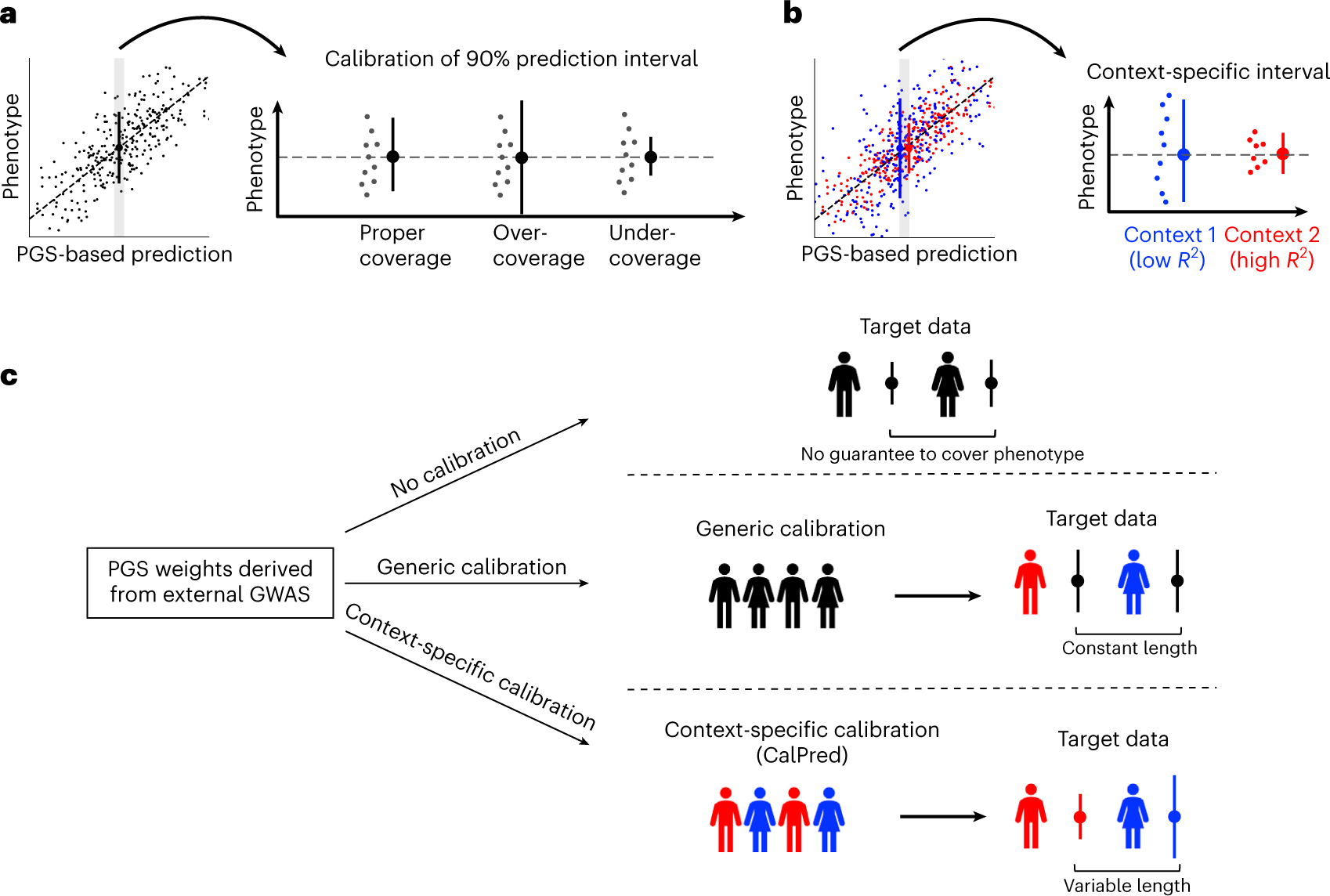
a, Calibration of prediction intervals. We consider a set of individuals with the same point prediction (shaded area, left; dashed horizontal line, right). Each dot denotes an individual’s phenotype value. Intervals with proper coverage cover the true phenotype at prespecified probability of 90%; intervals with over-coverage are incorrectly wide; intervals with under-coverage are incorrectly narrow. b, Context-specific calibration of prediction intervals. We consider two subpopulations in different contexts. Context 1 has lower prediction accuracy and therefore wider variation around the mean, while context 2 has higher prediction accuracy and therefore narrower variation around the mean. Context-specific intervals vary by context, providing intervals with proper coverage in each context. c, Different approaches for prediction intervals of PGS-based models. All approaches start with a set of predefined PGS weights derived from existing GWAS. ‘No calibration’: prediction intervals can be calculated using analytical formula without calibration data. However, these intervals are not guaranteed to be well calibrated. ‘Generic calibration’: these methods do not consider context information; they produce generic prediction intervals that are constant across individuals. ‘Context-specific calibration’: these methods leverage a set of calibration data to estimate the impact of each context to trait prediction accuracy; the estimated impact can then be used to generate prediction intervals for any target individuals matching in distribution with calibration data.

Next, we distinguish three categories of data. Training, used to perform GWAS and PGS weights estimation, often involves meta-analysis of multiple datasets where additional context adjustment is impractical due to data access limitations or unmeasured context variables. Calibration, used to calibrate PGS with respect to trait-relevant contexts, such as EHR-linked biobanks within medical systems, reflects the makeup of the patient population. Testing, with new individuals for whom prediction models will be employed (for example, patients within medical systems not currently involved in EHR-linked biobanks). Motivated by clinical implementation of PGS-based predictions in medical systems where EHR-linked biobanks already exist, we focus on the problem of using calibration data to provide multi-context calibration. We assume that the EHR-linked biobanks are reflective of future patients within the same medical system.

Context-specific prediction intervals are implemented with two components: (1) context-specific mean $\widehat{y_i}=\mathbb{E}\left[y_i\mid {\mathbf{c}}_i\right]$ as a function of context ${\mathbf{c}}_i$ for each individual $i$; we also include PGS–context interaction terms (PGS×C) to model varying PGS slope across contexts; (2) context-specific variance $\mathbb{E}\left[{\left(y_i-\widehat{y_i}\right)}^2\mid {\mathbf{c}}_i\right]=\mathrm{e}\mathrm{x}\mathrm{p}\left({\mathbf{c}}_i^{\mathrm{\top }}{\mathbf{\beta }}_{\sigma }\right)$, where ${\mathbf{c}}_i$ denotes contexts including age, sex, socioeconomic factors and genetic ancestry, and ${\mathbf{\beta }}_{\sigma }$ quantifies the unique impact of each context on variation of the prediction interval accounting for other contexts (Methods). Denoting prediction standard deviation (s.d.) as ${\hat{\sigma }}_i=\sqrt{\mathrm{e}\mathrm{x}\mathrm{p}({\mathbf{c}}_i^{\mathrm{\top }}{\stackrel{\mathbf{ˆ}}{\mathbf{\beta }}}_{\sigma })}$, 90% prediction intervals can be derived as $\left(\widehat{y_i}-1.645\times \widehat{{\sigma }_i},\widehat{y_i}+1.645\times \widehat{{\sigma }_i}\right)$. Our approach builds upon existing models for heteroscedasticity in probabilistic forecasting^35–39. Existing works incorporate variable residual variances across different subsets of data (that is, contexts in our case) in addition to modeling prediction mean in standard regression analysis. Within genetics literature, such models have been used to detect genotypes associated with phenotype variability^40–42. We build on such methods toward modeling PGS variable accuracy across contexts.

Widespread context-specific PGS accuracy across populations

Although PGS accuracy has been shown to vary across selected traits and contexts^5,11–13, its pervasiveness remains unclear. We analyzed two large-scale biobanks in the United Kingdom and the United States (UK Biobank and All of Us) comprising >600,000 individuals spanning a wide range of contexts. We trained PGS for 72 traits in individuals previously annotated as ‘white British’²⁸ (WB) from UK Biobank and evaluated these PGS in independent testing data from UK Biobank and All of Us. We focused on 11 contexts that span age, sex, socioeconomic factors such as educational attainment and genetic ancestry (we used top two genetic principal components (PCs) to represent major axes of genetic variation; see ‘Population descriptor usage’ section in Methods). We used relative $\mathrm{\Delta }{R}^2$ to quantify the impact of context to PGS accuracy, defined as $\frac{R_{\text{top}\text{quintile}}^2-R_{\text{bottom}\text{quintile}}^2}{R_{\text{all}}^2}$, where $R_{\text{[subset]}}^2$ denotes $R^2$ between PGS and residual phenotype computed in a given range of the context variable (top/bottom quintile as subsets for continuous contexts; binary subgroups as subsets for binary contexts). We found widespread context-specific PGS accuracy across all traits and contexts studied (Methods, Fig. 2, Supplementary Figs. 1 and 2 and Supplementary Tables 1 and 2).

Fig. 2 |. Widespread context-specific PGS prediction accuracy in UK Biobank.

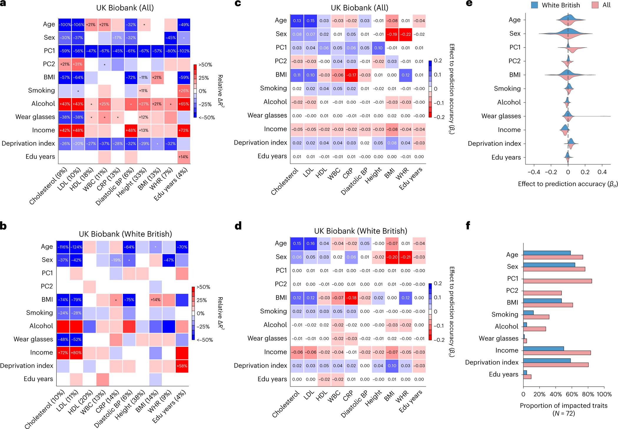
a,b, Heatmaps for context-specific PGS accuracy for all individuals (a) and WB individuals (b). Each row denotes a context and each column denotes a trait; the squared correlation between PGS and residual phenotype ($R^2$) is shown in parentheses. Heatmap color denotes the PGS phenotype relative $\mathrm{\Delta }{R}^2$ (defined as $\frac{R_{\text{group}1}^2-R_{\text{group}2}^2}{R_{\text{all}}^2}$), where $R_{\text{[subset]}}^2$ represents $R^2$ computed in a given range of the context variable. For continuous contexts, relative $\mathrm{\Delta }{R}^2$ denotes differences of top quintile minus bottom quintile; for binary contexts (including sex, smoking, wear glasses and alcohol), relative $\mathrm{\Delta }{R}^2$ denotes differences of male minus female, smoking minus not smoking, wearing glasses minus not wearing glasses, drinking alcohol minus not drinking alcohol (these orders were arbitrarily chosen). Numerical values of relative $R^2$ differences are displayed for PGS–context pairs with statistically significant differences (multiple testing correction for all 10 × 11 PGS–context pairs in this figure; two-sided P < 0.05/(10 × 11)). *PGS–context pairs with nominally significant differences (multiple testing correction for 11 contexts; two-sided P < 0.05/11). c,d, Heatmaps of effects to prediction accuracy in CalPred model (estimated ${\beta }_{\sigma }$) for all individuals (c) and WB individuals (d). Colormaps were inversed to those of a and b to reflect that positive ${\beta }_{\sigma }$ corresponds to lower prediction accuracy and vice versa. e, Distribution of estimated ${\beta }_{\sigma }$ in the CalPred model for each context across traits. f, Number of significantly impacted traits by each context (two-sided P < 0.05/(72 × 11)). CRP, C-reactive protein; BP, blood pressure; Edu, education.

Context-specific accuracy in UK Biobank

All 72 traits had at least one context impacting their accuracy in UK Biobank data; 264 (out of 792) PGS–context pairs had significant variable accuracy (P < 0.05/(72 × 11); Methods). Genetic ancestry had the most widespread impact on PGS accuracy: 70 of 72 traits had significant differences in PGS accuracy, with an average relative $\mathrm{\Delta }{R}^2$ of −46% between top and bottom PC1 quintiles (Supplementary Fig. 3). Socioeconomic contexts also significantly impacted PGS accuracy; PGS accuracy significantly differed for 62 traits, with an average relative $\mathrm{\Delta }{R}^2$ of −23% between top and bottom deprivation index quintiles. The direction of context’s impact depended on the trait being studied. For example, age significantly impacted 20 traits; rather than consistently increasing or decreasing accuracy, an older age led to increased accuracy for 14 traits (for example, high-density lipoprotein cholesterol (HDL) and white blood cell count (WBC) in Fig. 2) and to decreased accuracy for 6 traits (for example, LDL).

The widespread context specificity remained when testing data were matched to training data by genetic ancestry (Fig. 2). A total of 21 (out of 72) PGS had at least one context significantly impacting their prediction accuracy; 42 PGS–context pairs had significant variable accuracy (P < 0.05/(72 × 11)). We replicated previously reported variable PGS accuracy in WB individuals for diastolic blood pressure, body mass index, and ‘education years’ across contexts of sex, age and deprivation index¹¹. As an example, LDL was significantly impacted by six contexts in WB individuals, with age having the strongest impact (relative $\mathrm{\Delta }{R}^2$ was more than 100% between top and bottom age quintiles).

Next, we studied the unique impact of each context on variable PGS accuracy within CalPred model jointly accounting for all contexts (Methods and Fig. 2c,d). Context contribution to variable accuracy conditional on all other contexts was quantified with ${\beta }_{\sigma }$, where larger absolute ${\beta }_{\sigma }$ indicated more substantial variation in accuracy along a context variable (Methods). Effects of contexts to traits were largely independent. For example, both PC1 and deprivation index significantly impacted PGS accuracy for a range of traits in the joint model, indicating both had a unique contribution to variable PGS accuracy. We also found examples showing otherwise: the impact of the ‘wear glasses’ context on LDL accuracy can be explained by its correlation with age (Extended Data Fig. 1), while other contexts independently contributed to variable LDL accuracy. These results indicated the importance of jointly considering all measured contexts to correctly assess the unique contribution of each context. We found that contexts including sex, age, income and deprivation index had comparable impact on accuracy as genetic ancestry (Fig. 2e,f). The distribution of estimated effects of ${\beta }_{\sigma }$ suggested predominantly higher prediction accuracy for individuals with higher income and lower deprivation indices, partly explained by different context distribution in training versus testing data: WB individuals had higher income and lower deprivation indices compared to the rest of the UK Biobank⁴³ (Extended Data Fig. 2). We noted two context–trait pairs with large differences between single-context and combined-context analysis results even within UK Biobank WB individuals (sex–body mass index (BMI) and sex–waist–hip ratio (WHR)). This is because single-context analysis uses population-level $R^2$ focusing on the predictive power of only PGS while combined-context analysis assesses the impact of context on phenotypical residual variance (Supplementary Note).

Context-specific accuracy in All of Us

We next turned to All of Us, a diverse biobank across the United States comprising more than 245,000 participants (Supplementary Fig. 3 and Extended Data Fig. 3). Due to challenges in phenotype matching across biobanks, we restricted the analysis to 12 PGS and 11 contexts matching the UK Biobank analyses (Methods). All PGS had at least one context impacting their accuracy (Fig. 3 and Supplementary Tables 3 and 4). A total of 89 PGS–context pairs were significant when considering all individuals, and 61 PGS–context pairs were significant when restricting to individuals with self-identified race/ethnicity (SIRE) as ‘white’ (‘white SIRE’) (P < 0.05/(12 × 11); Methods). Prediction of cholesterol and LDL was similarly impacted by a broad range of contexts. Prediction of ‘education years’ was impacted by contexts including age, BMI, employment and income, both when considering all individuals and considering the ‘white SIRE’ sample, consistent with the socioeconomic contexts influencing PGS of sociobehavioral traits such as education^11,44,45.

Fig. 3 |. Widespread context-specific PGS prediction accuracy in All of Us.

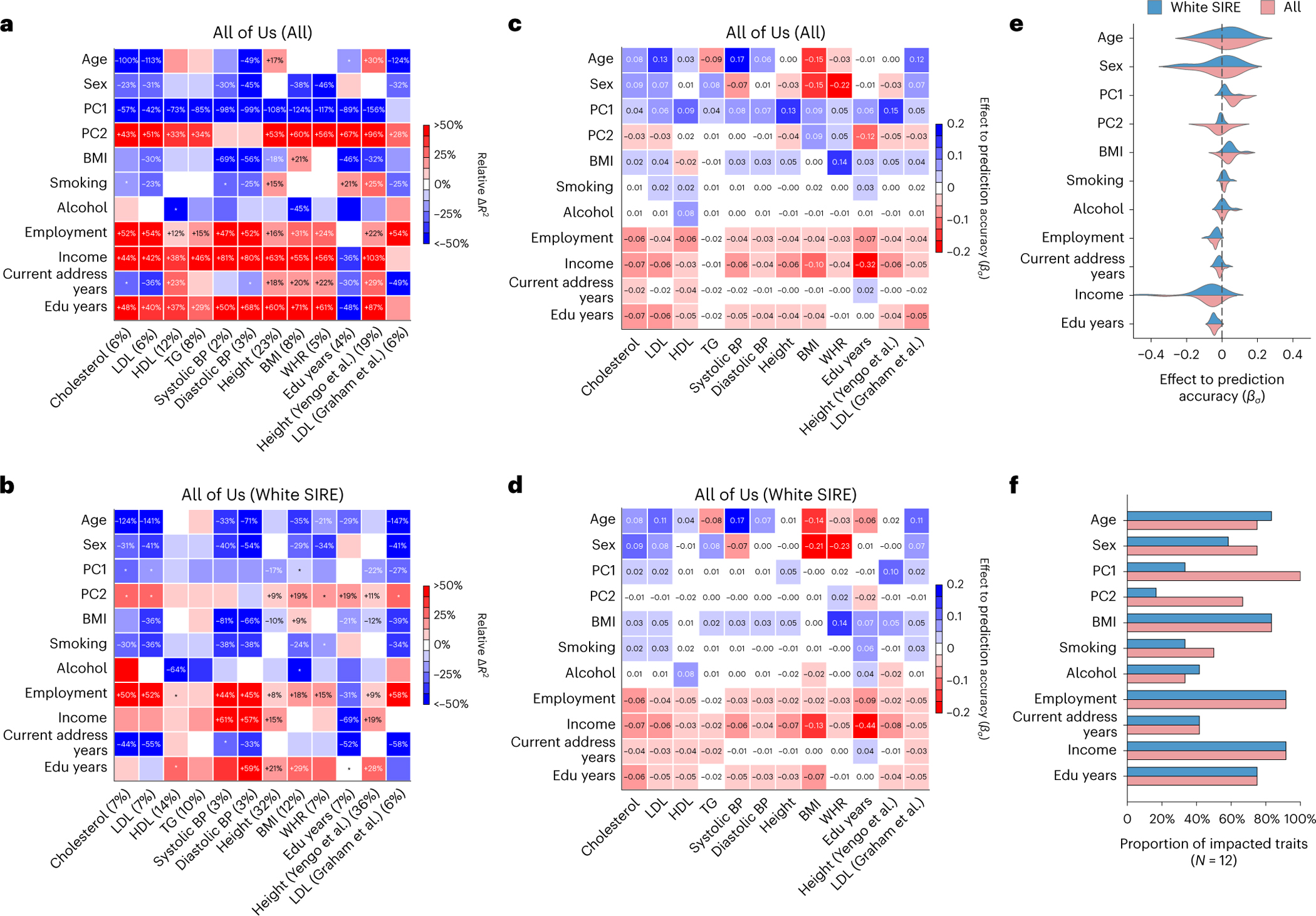
a,b, Heatmaps for context-specific PGS accuracy for all individuals (a) and white SIRE individuals (b). Each row denotes a context and each column denotes a trait; overall $R^2$ is shown in parentheses. Heatmap color denotes relative $\mathrm{\Delta }{R}^2$: differences of top quintile minus bottom quintile for continuous contexts and difference of male minus female for binary context of sex. Numerical values of relative $R^2$ differences are displayed for trait–context pairs with statistically significant differences (multiple testing correction for all 12 × 11 PGS–context pairs in this figure; two-sided P < 0.05/(12 × 11)). *PGS–context pairs that are displayed with nominally significant differences (multiple testing correction for 11 contexts; two-sided P < 0.05/11). c,d, Heatmaps of estimated ${\beta }_{\sigma }$ in CalPred model for all individuals (c) and white SIRE individuals (d). e, Distribution of estimated ${\beta }_{\sigma }$ in CalPred model for each context across traits. f, The number of significantly impacted traits by each context (with two-sided P < 0.05/(12 × 11)). BP, blood pressure; Edu, education; TG, triglycerides.

Interestingly, socioeconomic contexts had greater impact on context specificity in All of Us as compared to UK Biobank. For example, ‘education years’ context significantly impacted 9 out of 11 traits with average relative $\mathrm{\Delta }{R}^2=50\mathrm{\%}$, as compared to 2 out of 71 traits with average relative $\mathrm{\Delta }{R}^2=0.2\mathrm{\%}$ in UK Biobank (averaging across traits other than ‘education years’ itself). This may be explained by larger variation of ‘education years’ in the United States and/or ‘education years’ being more correlated with social determinants of health in the United States compared to the United Kingdom. When restricting analysis to a subset of individuals with more homogeneous genetic ancestry, the impact of ‘education years’ and income level was attenuated but remained significant; this is consistent with variable PGS accuracy across socioeconomic contexts being partially accounted for through their correlation with genetic ancestry (Extended Data Fig. 4).

For completeness we also evaluated PGS for height⁴⁶ and LDL⁴⁷ derived from multi-ancestry meta-analyses from PGS catalog⁴⁸ (Fig. 3). We found that multi-ancestry PGS did not alleviate widespread context-specific accuracy. Higher income, ‘education years’, better employment or lower BMI predominately led to higher prediction accuracy across traits (Fig. 3e,f). Additional secondary analyses assessing the consistency of fitted ${\beta }_{\sigma }$ coefficients across populations, as well as factors explaining context-specificity patterns, are reported in Supplementary Figs. 4–6.

CalPred is calibrated across contexts in simulations

Having shown pervasive context specificity of PGS accuracy, we next turned to CalPred to estimate context-specific prediction intervals accounting for context- and trait-specific variable accuracy (Methods). We performed simulations to evaluate calibration of CalPred in the presence of gene-by-context interactions^16,49. For quantitative traits, we simulated individuals in two contexts with different heritability and an imperfect genetic correlation (the first context is used to train PGS; Methods and Fig. 4a). Due to genetic heterogeneity, PGS weights derived in the first context were not portable to the second context, producing a biased phenotype–PGS regression slope and prediction intervals with deflated coverage. With CalPred, prediction mean was calibrated via PGS×C terms; prediction interval lengths were adjusted to reflect different prediction precision across two contexts. For disease traits, we simulated individuals in two contexts under a liability threshold model with different disease prevalence and an imperfect genetic correlation (Fig. 4b and Methods). We first predicted disease probability with a logistic regression model for all individuals in both contexts, using PGS weights derived from the first context. As expected, this model ignoring context information was miscalibrated overall in each context. By incorporating PGS, PGS×C interaction and context variables, we determined disease risk predictions were then calibrated within and across contexts. We also simulated other scenarios of gene–context interactions for both quantitative and disease traits and verified that our framework produced calibrated predictions (Extended Data Figs. 5 and 6).

Fig. 4 |. Simulation studies with gene–context interactions.

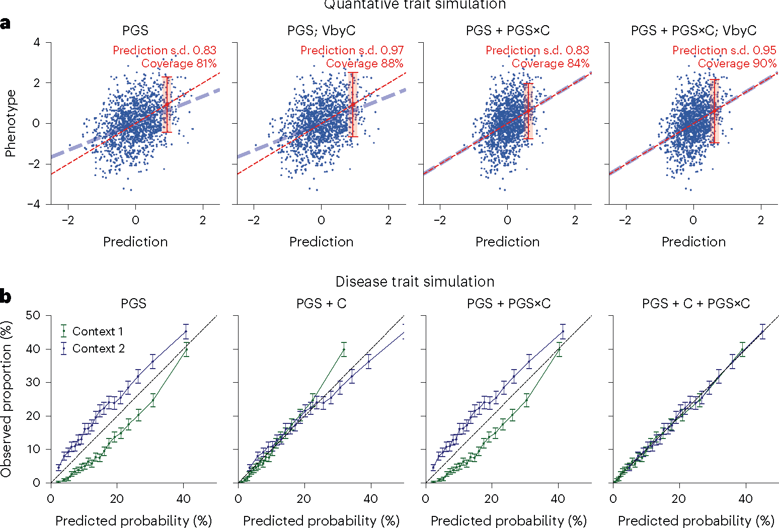
a, For quantitative traits, we simulated traits for individuals in two contexts with 0.7 cross-context genetic correlation and heritability of 0.5/0.4, respectively, in two contexts. PGS weights were trained in the first context and applied in the second context. We showed results for predictions in the second context using four combinations of approaches to model prediction mean (using PGS or PGS+PGS×C) and prediction variance (with or without VbyC). We did not simulate effects of context variables to phenotype and therefore results using ‘PGS + C’ and ‘PGS + C+PGS×C’ would yield same results as ‘PGS’ and therefore were not included. Dashed blue line denotes the best fit to data; dashed red line denotes model predictions; red error bar denotes the CalPred 90% prediction interval for individual at top 5% quantile of PGS. Prediction interval coverage was evaluated within data in top PGS decile. Additional details can be found in Extended Data Fig. 5 and Methods. b, For disease traits, we simulated diseases for individuals in two contexts under a liability threshold model with 0.5 heritability, 0.7 cross-context genetic correlation and disease prevalence of 10%/20%, respectively, in two contexts (blue and green lines). Disease probability was predicted using four sets of predictors: (1) PGS; (2) PGS and context variables (PGS + C); (3) PGS and PGS×C (PGS + PGS×C); (4) PGS, context variables and PGS×C (PGS + C + PGS×C). VbyC led to similar results. Error bars denote observed disease proportions and their 95% confidence intervals for each predicted probability bin (n = 2,000 individuals for each error bar). Additional details can be found in Extended Data Fig. 6 and Methods.

We next evaluated CalPred in simulations where prediction accuracy varies across contexts similar to real data^5,7,11 (Fig. 5 and Methods). We assessed calibration of prediction intervals both at the overall level and within each context subgroup (Methods). First, generic prediction intervals without context-specific adjustment had severe over-/under-coverage within each context subgroup stratified by PC1, age or sex. As expected, bias of coverage tracked closely with accuracy across contexts. Second, CalPred context-specific prediction intervals were calibrated across contexts, by incorporating context-specific prediction accuracy in the interval estimation. We also performed simulations to find if CalPred performance depended on calibration sample size $N_{\text{cal}}>500$ for accurate model fitting and an appropriate set of contexts in calibration (Extended Data Fig. 7). Parameter estimation of ${\beta }_{\sigma }$ was accurate with correctly specified model and robust with model misspecification (Supplementary Fig. 7). Overall, simulation results demonstrated that CalPred produces well-calibrated prediction intervals when contexts are measured and present in the data and highlighted the importance of comprehensive profiling of relevant context information.

Fig. 5 |. Simulation studies with multiple contexts.

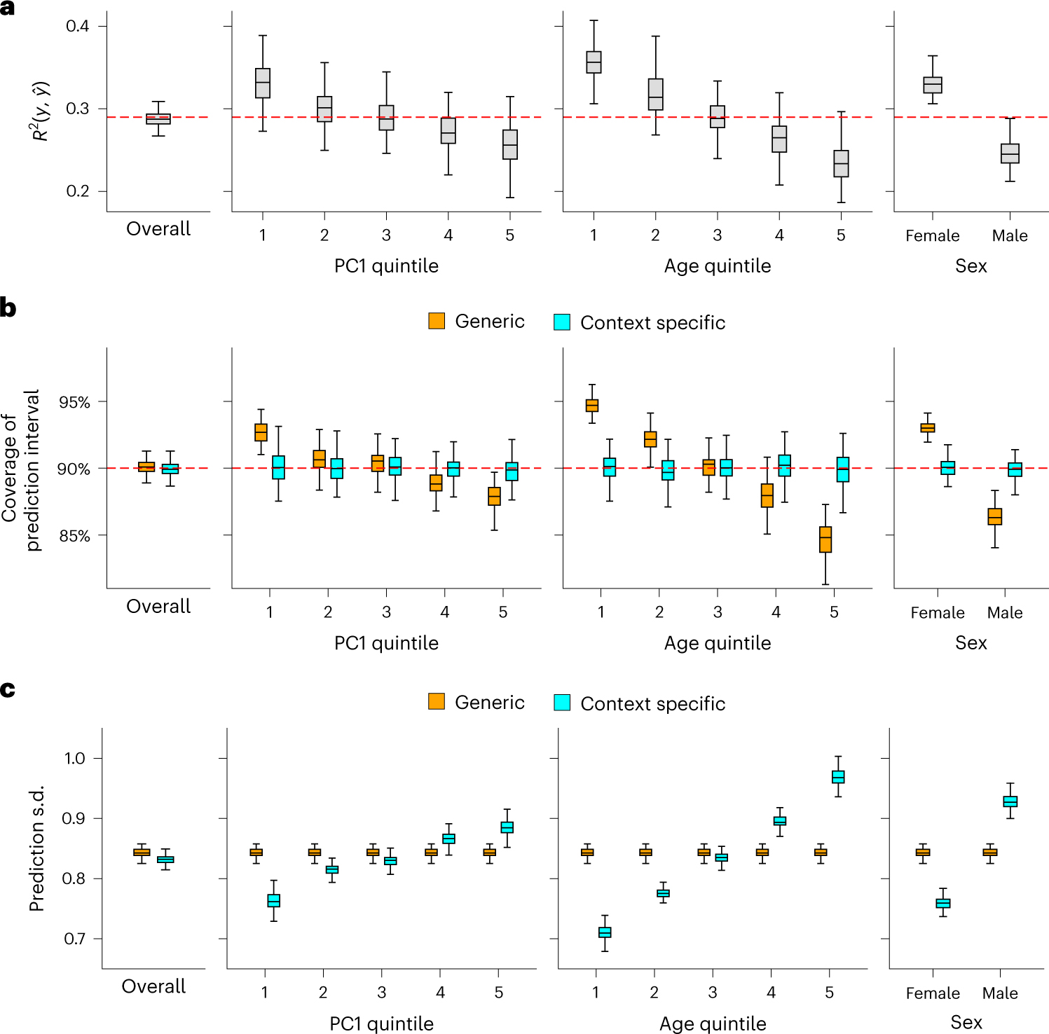
Simulations were performed to reflect scenarios where individuals have variable prediction accuracy by genetic PC1, age and sex. For each simulation, we first trained a calibration model using a random set of 5,000 training individuals and then evaluated resulting prediction intervals on 5,000 target individuals (Methods). a, Prediction $R^2$ between $y$ and $\hat{y}$ in simulated data both at the overall level and in each context subgroup. b, Coverage of generic (orange) versus context-specific (blue) 90% prediction intervals evaluated in each context subgroup. Generic intervals were obtained by applying CalPred without context information; context-specific intervals were obtained by applying CalPred together with context information. c, Average length of generic versus context-specific prediction s.d. in each context. Across a, b and c, each box plot contains $R^2/\mathrm{c}\mathrm{o}\mathrm{v}\mathrm{e}\mathrm{r}\mathrm{a}\mathrm{g}\mathrm{e}/\mathrm{a}\mathrm{v}\mathrm{e}\mathrm{r}\mathrm{a}\mathrm{g}\mathrm{e}\mathrm{l}\mathrm{e}\mathrm{n}\mathrm{g}\mathrm{t}\mathrm{h}$ evaluated across 100 simulations (n = 100 points for each box); the center corresponds to the median, the box represents the first and third quartiles of the points, and the whiskers represent the minimum and maximum points located within 1.5× interquartile range from the first and third quartiles, respectively.

CalPred yields calibrated context-specific predictions

We applied CalPred to produce context-specific prediction intervals for a wide range of quantitative traits. We first performed several analyses in All of Us to investigate best practices to model quantitative traits. We examined effects of PGS, context variables and PGS×C for trait prediction and found that PGS contributed the most in explaining trait variation (cross-trait average standardized effects with magnitudes of 0.23 compared to 0.22 of sex and 0.14 of BMI, the second and third largest contributors). PGS×C had significant contributions but with smaller effects than those from context variable themselves (Extended Data Fig. 8). Notably, inclusion of PGS substantially increased inter-individual variation in prediction s.d., suggesting that PGS is an important source of variation in prediction accuracy (Extended Data Fig. 9). PGS×C and modeling variance by contexts (VbyC) components had additive contribution in improving model fitting, capturing independent aspects of traits (Supplementary Figs. 8–10).

We focused on LDL, an important risk factor of cardiovascular disease⁴⁷. Calibration by context is particularly important because LDL prediction accuracy was impacted by many contexts, with the largest impact made from age (Figs. 2 and 3). We modeled prediction mean using PGS together with age, sex and genetic ancestry, and modeled context-specific prediction intervals using the set of contexts in Figs. 2 and 3 (Methods). LDL prediction accuracy decreased with age ($R^2=18\mathrm{\%}$ in youngest quintile versus $R^2=11\mathrm{\%}$ in oldest quintile; Fig. 6a). Generic prediction intervals were miscalibrated with coverage of 93% and 86% for youngest and oldest quintiles instead of the nominal level of 90%. In contrast, context-specific prediction intervals had the expected 90% coverage across all considered contexts. This resulted from varying prediction interval length by context, with a wider interval compensating for lower prediction accuracy. For example, as CalPred estimated a positive impact of age to prediction uncertainty (${\beta }_{\sigma }=0.15$; P < 10⁻³⁰), individuals in youngest/oldest age quintiles had average prediction s.d. of 27.4 versus 34.3 mg dl⁻¹ (25% difference; Supplementary Fig. 11 and Methods). These findings were replicated in All of Us and in other traits (Supplementary Figs. 12 and 13), where $R^2$ varied across contexts and context-specific prediction intervals achieved well calibration across contexts providing per-individual accuracy metrics (Supplementary Fig. 14). Next, we sought to examine the joint contribution of all considered contexts to variable prediction s.d. (instead of separately considering age, PC1 or sex; Fig. 6b). Context-specific accuracy was more pronounced by ranking individuals by prediction s.d. accounting for impact of all contexts (prediction s.d. ranged approximately from 20 mg dl⁻¹ to 45 mg dl⁻¹; Fig. 6b): we detected a 44% difference comparing individuals in bottom and top deciles of prediction s.d. (25.2 mg dl⁻¹ versus 36.5 mg dl⁻¹; Fig. 6c and Supplementary Figs. 15 and 16). This implied that individuals in top prediction s.d. decile (characterized by contexts of male, increased PC1 and age; Fig. 2c) need to have prediction interval widths increased by 44% compared to those in bottom decile.

Fig. 6 |. CalPred PGS calibration of LDL in UK Biobank.

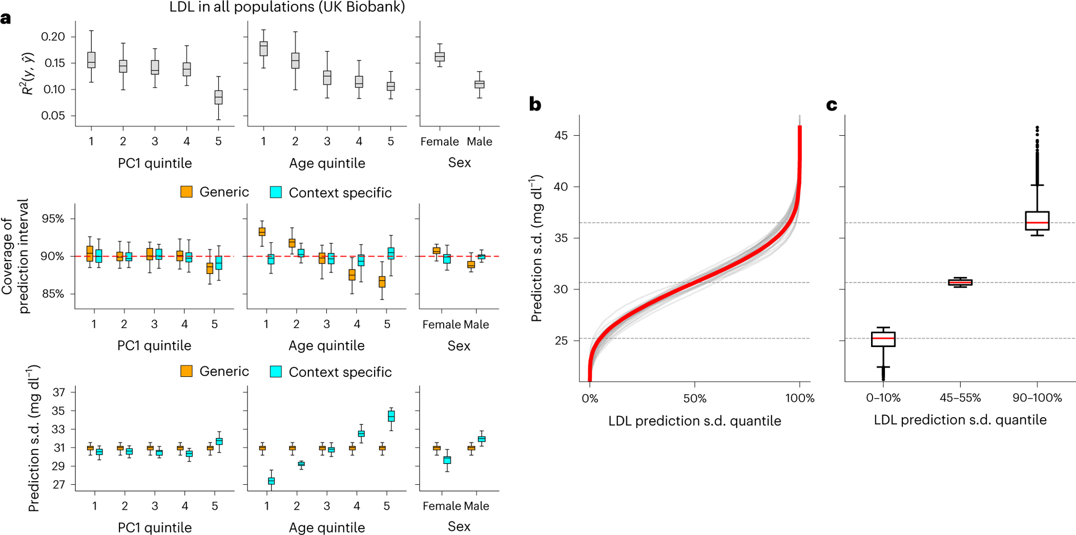
a, Top: prediction $R^2$ between phenotype and point predictions (incorporating PGS and other covariates) in each subgroup of individuals stratified by context ($R^2$ evaluated across all individuals is 0.147). Middle: coverage of generic (orange) versus context-specific (blue) 90% prediction intervals evaluated in each context subgroup. Generic intervals were obtained by applying CalPred without context information; context-specific intervals were obtained by applying CalPred together with context information. Bottom: average length of generic versus context-specific 90% prediction intervals in each context. Each box plot contains $R^2$, coverage or average length across 30 random samples with each sample of 5,000 training and 5,000 target individuals (n = 30 points for each box). b, Ordered LDL prediction s.d. in the unit of mg dl⁻¹. Gray lines denote prediction s.d. obtained with random sample of 5,000 training and applied to 5,000 target individuals. Red lines denote prediction s.d. obtained from all individuals. c, Box plots of results in b from individuals of LDL prediction s.d. quantile of 0–10%, 45–55% and 90–100% (n = 110,000 individuals in total). For box plots in both a and c, the center corresponds to the median, the box represents the first and third quartiles of the points, and the whiskers represent the minimum and maximum points located within 1.5× interquartile range from the first and third quartiles, respectively.

Extending analysis accounting for all contexts to all traits in UK Biobank and All of Us, we determined a widespread large variation of context-specific prediction intervals across traits (Fig. 7 and Supplementary Fig. 17). Average differences between top and bottom prediction s.d. deciles across traits were 30% and 47%, respectively, for UK Biobank and All of Us. Comparing across two datasets, BMI, LDL and cholesterol were more heavily influenced by context than average, while diastolic blood pressure and HDL were less impacted, suggesting trait-specific susceptibility to context-specific accuracy. There were cases where context specificity of the same trait was drastically different across datasets. For example, prediction s.d. differences for predicting ‘education years’ were 94% in All of Us versus 10% in UK Biobank. This disparity probably reflected the more diverse distribution of ‘education years’ and other social determinants of health in the US population sampled in All of Us (Figs. 2 and 3). Such differences between datasets highlight that context specificity can be population specific and the need to consider characteristics of different populations in calibration.

Fig. 7 |. Variation of prediction s.d. accounting for all contexts.

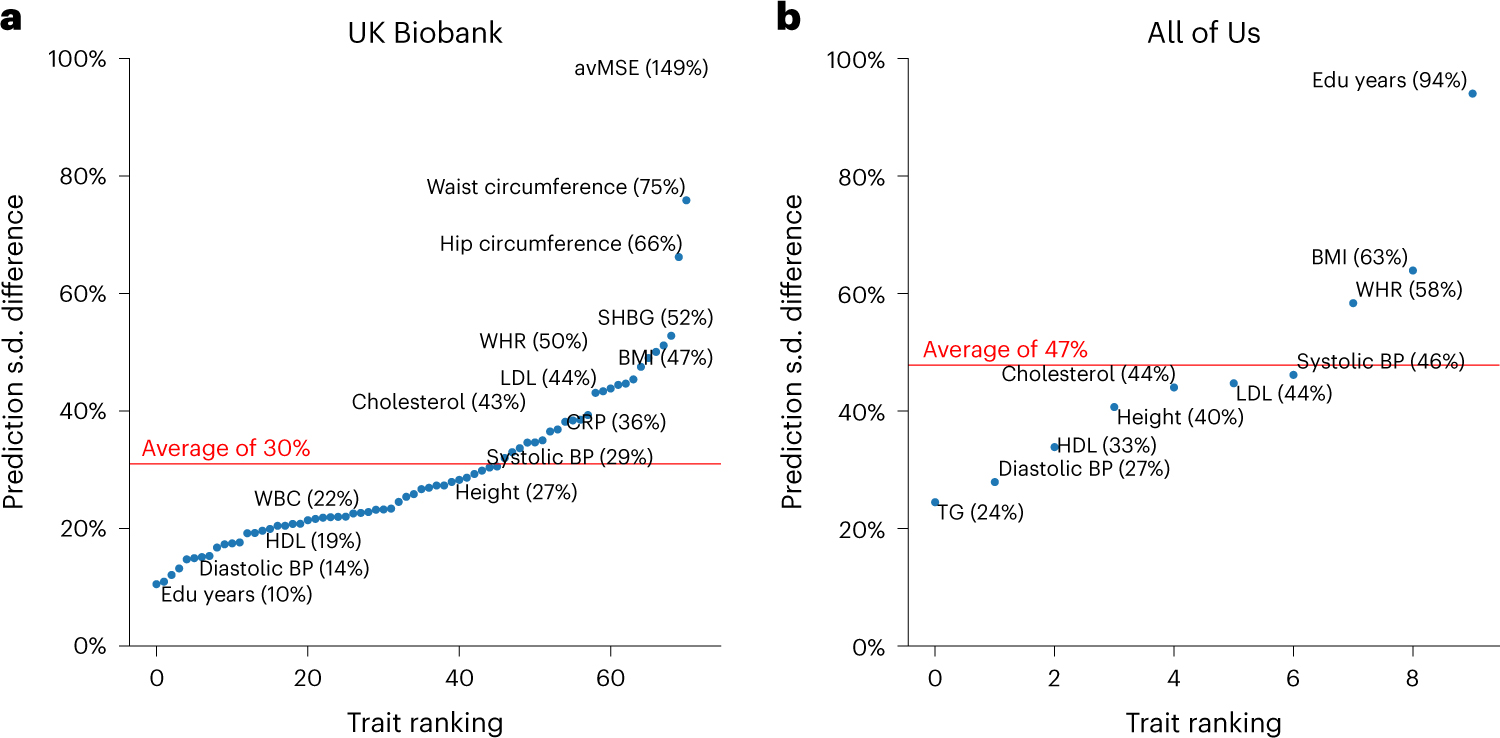
a,b, Relative difference of prediction s.d. between top and bottom prediction s.d. deciles (90–100% versus 0–10%) for all traits in UK Biobank (a) and All of Us (b). Traits are ranked by prediction s.d. The difference is calculated with the median prediction s.d. within decile of individuals with highest prediction s.d. $s_{\mathrm{d}1}$ and decile of individuals with lowest prediction s.d. $s_{\mathrm{d}10}$ using $\left(\frac{s_{\mathrm{d}1}-s_{\mathrm{d}10}}{s_{\mathrm{d}10}}-1\right)\times 100\mathrm{\%}$. The trait with the highest prediction s.d. difference was average mean spherical equivalent (avMSE), a measure of refractive error that was impacted the most by ‘wear glasses’ context. Individuals who wore glasses had a much higher PGS phenotype $R^2$ than those who did not, probably due to the reduced variation in avMSE phenotypes among individuals who did not wear glasses. Red lines denote the average prediction s.d. difference across traits within each dataset. SHBG, sex hormone binding globulin; CRP, C-reactive protein; BP, blood pressure; TG, triglycerides; Edu years, ‘education years’.

We next investigated disease risk prediction for four well-powered heritable diseases: T2D⁵⁰, coronary artery disease⁵¹, prostate cancer⁵² and breast cancer⁵³ (Extended Data Fig. 10). We first considered a baseline model using logistic regression to predict disease probability with PGS, age, sex, BMI and top ten PCs as predictors (Methods). We evaluated calibration of predicted disease risk—whether predicted probability aligned with the observed disease rate. While baseline model predictions were calibrated at an aggregate level, they were miscalibrated within specific contexts (Fig. 8a). For example, among individuals with a predicted T2D risk of approximately 30% (25–35%, N = 4,662), the observed proportion with T2D was 30.9% (standard error (s.e.), 0.7%). However, this proportion varied significantly with individual’s ‘annual household income’: 32.7% (s.e., 2.0%) in the lowest income bracket (N = 562) had T2D, compared to only 18.1% (s.e., 2.3%) in the highest income bracket (N = 271); T2D risk was consistently underestimated for individuals of lower income and overestimated for individuals with higher income. The discrepancy suggests that a baseline model ignoring disease-relevant contexts produces severely miscalibrated probability estimates. We then used a logistic model to incorporate contexts, including ‘annual household income’ together with their interaction with PGS, to find that predicted disease risk was calibrated at the overall level and also within each income group; modeling variance by context for disease liability achieved similar calibration (Fig. 8b and Supplementary Figs. 18 and 19) and we discussed reasons explaining their similar performances (Methods). Overall, our results emphasize the importance of incorporating contexts into probability risk calibration to achieve calibrated predictions across all considered contexts.

Fig. 8 |. Calibration of T2D risk prediction across income groups.

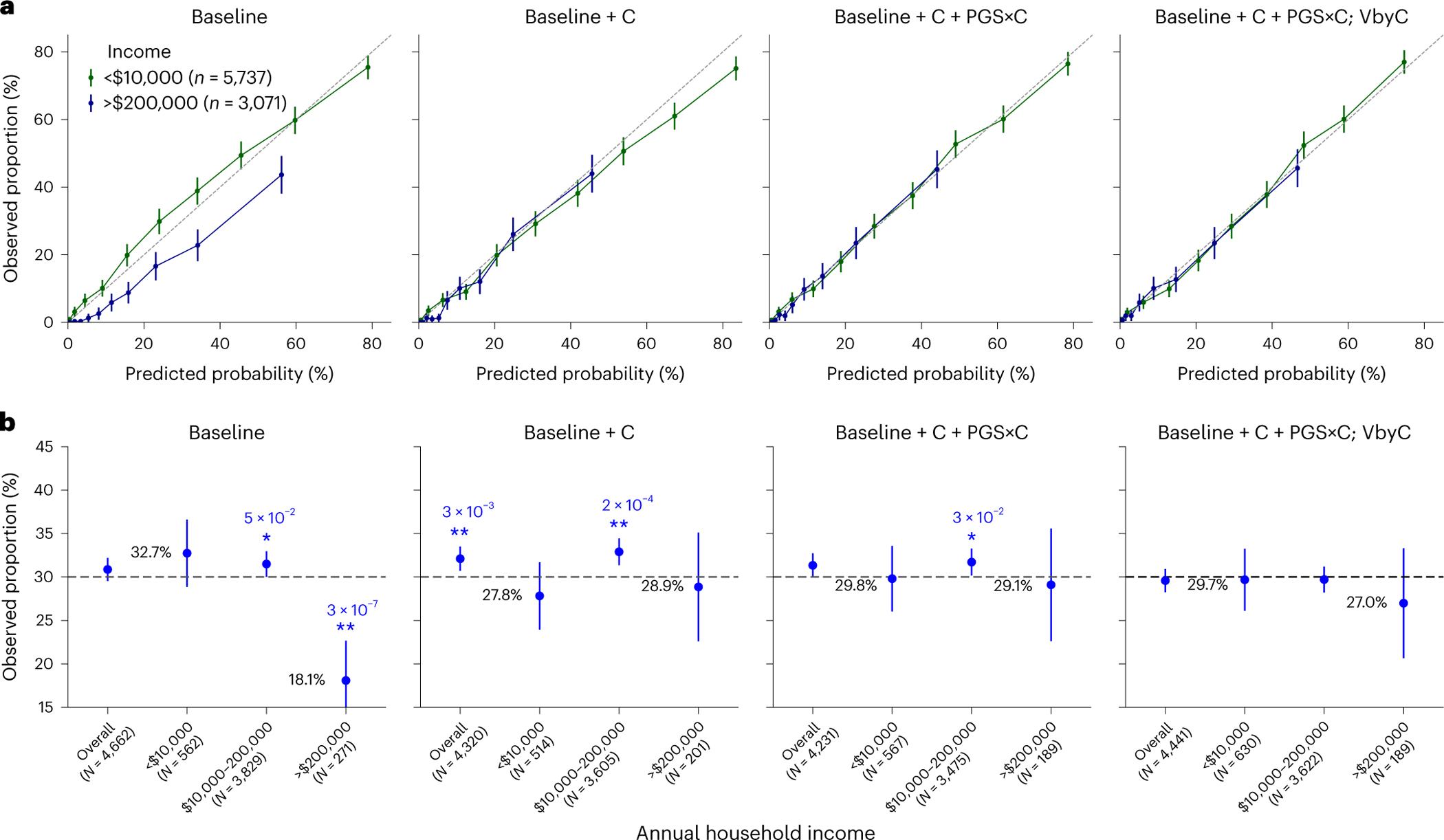
We compared four models for predicting T2D across all individuals in All of Us. ‘Baseline’ is the logistic regression model with PGS, age, sex, BMI and top ten PCs as predictors; ‘Baseline+C’ is the logistic regression model additionally including smoking status, drinking, employment, income, current address years and ‘education years’; ‘Baseline+C+PGS×C’ additionally includes PGS×C interactions; and ‘Baseline+C+PGS×C; VbyC’ additionally shows modeling variance by contexts within a liability threshold model. The dataset was evenly split into training and testing datasets. a, Observed proportion versus predicted probability of T2D for lowest (green) and highest (blue) income groups. Error bars denote the observed proportions and their 95% confidence intervals (number of total individuals shown in key). b, Observed proportion of individuals with T2D among individuals predicted with a predicted T2D risk of approximately 30% (25–35%) for baseline and calibrated models stratified by annual household income. Error bars denote the observed proportions and their 95% confidence intervals (number of individuals for each error bar is shown in parentheses). Numerical values of the observed proportions were shown in black fonts for ‘<$10,000’ and ‘>$200,000’ groups; * and ** denote statistical significance levels for deviations from the 30% predicted risk, with * indicating P < 0.05 and ** denoting P < 0.01, respectively (two-sided tests); numerical P values were also displayed.

Discussion

Our work adds to the literature of PGS-based prediction. We show that context-specific accuracy of PGS is highly pervasive across traits and biobanks with socioeconomic contexts often having larger impact than genetic ancestry^{5,11,13,23,54}. We introduce CalPred to estimate context-specific prediction intervals. Compared to other PGS calibration approaches, CalPred incorporates context information leveraging a calibration dataset (Supplementary Note). For quantitative traits, CalPred provides a framework to quantify individualized context-specific generalizability/portability of a given PGS. Prediction intervals can be interpreted as a reference range accounting for each individual’s contexts providing individual-level uncertainty metrics. For example, they can be used to identify individuals having PGS-based predictions with exceedingly high uncertainty and inform cases when it is not appropriate to report polygenic scoring results because of the high instability. For disease traits, we found models that overlooked context information resulting in miscalibrated disease probability predictions in the presence of gene–context interactions. Such miscalibrations are problematic if they lead to over-/under-diagnosis for individuals across socioeconomic context groups. To address this, we incorporated context variables and PGS×C interactions in PGS-based predictions, which led to calibrated predictions across contexts.

We note several limitations of our work. First, we motivated our approach for clinical implementation using continuous biomarkers and focused on LDL as an example continuous lab value with clinical application. Other biomarkers to consider could be prostate-specific antigen currently employed for patient stratification for biopsies and prostate cancer diagnosis. Recent work has highlighted incorporating genetically predicted prostate-specific antigen levels improves clinical utility by reducing unnecessary biopsies and improving detection of aggressive form of prostate cancer⁵⁵. Therefore, lab values form a useful system for prediction method development that may have clinical implications; actual clinical utility requires thorough implementation considering clinical decision processes. Second, CalPred requires calibration data that match in distribution with the target data, including both distribution of contexts and their impact to traits. Otherwise, there may be bias in target samples underrepresented in calibration data. Meanwhile, PGS weights do not need to be trained from the same population as the testing population. Third, comprehensive profiling of context information is fundamental in calibration and interpreting results. In our simulation studies, missing contexts prevent proper calibration of PGS. In our T2D analysis, ‘annual household income’ is probably a proxy of contexts such as diet and physical exercise that are more directly relevant to T2D. Therefore, we advocate standardized and comprehensive profiling of contexts across biobanks to quantify the role of contexts to PGS accuracy. Relatedly, GWAS data collection needs to prioritize diversity not only in genetic ancestry, but also across socioeconomic contexts. Fourth, context-specific accuracy can arise due to biological genetic effects differences across contexts such as gene-by-age and gene-by-sex interactions, or because of statistical differences of minor allele frequency/linkage disequilibrium patterns contributing to a substantial proportion of PGS performance differences across genetic ancestry. Disentangling various aspects driving context-specific accuracy is an ongoing research direction^11,16,49. Fifth, this work has primarily focused on the impact of PGS on the variability of prediction intervals across contexts. However, it is important to note that variable accuracy of other predictors and variable phenotypic variance also contribute to our findings. The results presented here regarding variable prediction accuracy should be attributed to the collective impact of all predictors, rather than solely to PGS. While we have determined the substantial contribution of PGS to variable accuracy, further quantifying the relative contributions of each predictor is an important future direction.

Online content

Any methods, additional references, Nature Portfolio reporting summaries, source data, extended data, supplementary information, acknowledgements, peer review information; details of author contributions and competing interests; and statements of data and code availability are available at https://doi.org/10.1038/s41588-024-01792-w.

Methods

Ethical approval

This research complies with all relevant ethical regulations. Ethics committee/institutional research board of UK Biobank gave ethical approval for collection of the UK Biobank data (https://www.ukbiobank.ac.uk/learn-more-about-uk-biobank/about-us/ethics). Approval to use UK Biobank at an individual level in this work was obtained under application 33297 at http://www.ukbiobank.ac.uk. Ethics committee/institutional research board of All of Us gave ethical approval for collection of All of Us data (https://allofus.nih.gov/about/who-we-are/institutional-review-board-irb-of-all-of-us-research-program). Approval to use All of Us controlled tier data in this work was obtained through application at https://www.researchallofus.org.

Constructing calibrated and context-specific prediction intervals

We first provide an overview of CalPred framework. CalPred takes as input pretrained PGS weights, genotype, phenotype and contexts to train a calibration model producing calibrated and context-specific prediction intervals for target individuals. We consider a calibration dataset with $N_{\text{cal}}$ individuals. For each individual $i=1,\dots ,N_{\text{cal}}$, we have a genotype vector ${\mathbf{g}}_i\in \{0,1,2{\}}^M$ with multiple ($M$) single-nucleotide polymorphisms (SNPs) and phenotype $y_i$. Using pretrained PGS weights for a given trait ${\mathbf{\beta }}_g\in {\mathbb{R}}^M$, we calculate PGS in calibration data with ${\mathbf{g}}_i^{\mathrm{\top }}{\mathbf{\beta }}_g$. PGS and other contexts including age, sex, genetic ancestry and socioeconomic factors compose each individual $i$’s contexts ${\mathbf{c}}_i$ (all ‘1’ intercepts are also included). Phenotypes are modeled as

$$y_i=𝒩\left(\mu \left({\mathbf{c}}_i\right),{\sigma }^2\left({\mathbf{c}}_i\right)\right),i=1,\dots ,N_{\text{cal}}$$

$$\mu \left({\mathbf{c}}_i\right)={\mathbf{c}}_i^{\mathrm{\top }}{\mathbf{\beta }}_{\mu },{\sigma }^2\left({\mathbf{c}}_i\right)=\exp \left({\mathbf{c}}_i^{\mathrm{\top }}{\mathbf{\beta }}_{\sigma }\right).$$

There are two main components:

• $\mu \left({\mathbf{c}}_i\right)={\mathbf{c}}_i^{\mathrm{\top }}{\mathbf{\beta }}_{\mu }$ models the baseline prediction mean using predictors of PGS, contexts, as well as PGS×C.

• ${\sigma }^2\left({\mathbf{c}}_i\right)=\mathrm{e}\mathrm{x}\mathrm{p}\left({\mathbf{c}}_i^{\mathrm{\top }}{\mathbf{\beta }}_{\sigma }\right)$ models context-specific variance of $y$ around prediction mean. Differential prediction accuracy across contexts lead to variable variance around prediction mean across contexts. The use of exp (·) is to ensure that the variance term ≥0. PGS×C terms are not included for ease of interpretation.

We estimate ${\mathbf{\beta }}_{\mu }$, ${\mathbf{\beta }}_{\sigma }$ leveraging calibration data using restricted maximum likelihood for linear model with heteroskedasticity⁵⁶ (statmod v1.5.0 (ref. 57)). Individual-specific predictive distribution $𝒩(\hat{\mu }({\mathbf{c}}_i)={\mathbf{c}}_i^{\mathrm{\top }}{\stackrel{\mathbf{ˆ}}{\mathbf{\beta }}}_{\mu },{\hat{\sigma }}^2({\mathbf{c}}_i)=\mathrm{e}\mathrm{x}\mathrm{p}({\mathbf{c}}_i^{\mathrm{\top }}{\stackrel{\mathbf{ˆ}}{\mathbf{\beta }}}_{\sigma }))$ can be generated for any target individual ${\mathbf{c}}_i$ using the fitted ${\stackrel{\mathbf{ˆ}}{\mathbf{\beta }}}_{\mu }$, ${\stackrel{\mathbf{ˆ}}{\mathbf{\beta }}}_{\sigma }$. The corresponding $\alpha$-level prediction interval (for example, $\alpha =90\mathrm{\%}$ for 90% prediction interval) is $\left[\hat{\mu }\left({\mathbf{c}}_i\right)-{\Phi }^{-1}\left(1-\frac{\alpha }{2}\right)\hat{\sigma }\left({\mathbf{c}}_i\right),\hat{\mu }\left({\mathbf{c}}_i\right)+{\Phi }^{-1}\left(1-\frac{\alpha }{2}\right)\hat{\sigma }\left({\mathbf{c}}_i\right)\right]$, where ${\Phi }^{-1}$ is the inverse cumulative distribution function of a standard normal distribution (for example, ${\Phi }^{-1}\left(1-\frac{\alpha }{2}\right)=1.645$ for 90% prediction interval). With moderate sample size for calibration data (for example, $N_{\text{cal}}>500$ as validated in our simulation studies), such models can be estimated with high precision.

Quantile normalization for nonnormal phenotype distribution.

In the above, we have assumed that prediction intervals can be modeled as a Gaussian distribution, which may not be valid for every phenotype. For robust implementation in real data, we apply a transformation function $Q(\cdot )$ to $y$ with rank-based inverse normal transformation such that $Q\left(y\right)$ follows a normal distribution; $Q\left(y\right)$ can then be modeled using methods described above. Fitted prediction intervals can then be transformed back into the original $y$ space using $Q^{-1}\left(y\right)$.

Model for disease trait within the liability threshold model.

CalPred model can be extended for disease traits. We first use CalPred to model continuous disease liability $y^{\text{liab}}=𝒩\left(\mu \left(\mathbf{c}\right),{\sigma }^2\left(\mathbf{c}\right)\right)$, and then integrate out scenarios where disease liability is above the threshold $P(y=1)=\Phi \left(y^{\text{liab}}>0\right)=\Phi \left(\frac{\mu (\mathbf{c})}{\sigma (\mathbf{c})}\right)$, where $\Phi (\cdot )$ is a link function used in logistic or probit regression. Intuitively, this maps the continuous liability into disease risk while accounting for liability uncertainty. Disease trait probability can be alternatively modeled using a logistic regression model $P(y=1)=\Phi \left({\mathbf{c}}^{\mathrm{\top }}{\mathbf{\beta }}_{\text{logistic}}\right)$. In real data analysis (Fig. 8 and Supplementary Fig. 19), we did not observe substantial improvement of CalPred model over logistic linear model. To explain this, comparing logistic regression model $P(y=1)=\Phi \left(\frac{\mu (\mathbf{c})}{\sigma (\mathbf{c})}\right)$, we note that ${\mathbf{c}}^{\mathrm{\top }}{\mathbf{\beta }}_{\text{logistic}}$ can be seen as first-order terms in Taylor expansion approximating $\frac{\mu (\mathbf{c})}{\sigma (\mathbf{c})}$. Therefore, our observation is explained by the fact that linear logistic regression model is a good approximation of CalPred disease model.

Quantifying context-specific ${\mathit{R}}^2$ of PGS

We quantify context-specific prediction accuracy ($R^2$) of PGS, that is, to what extent PGS have variable prediction accuracy across contexts (including age, sex, genetic ancestry, socioeconomic factors that can influence traits⁵⁸). Identification of contexts contributing to variable prediction accuracy is important in constructing calibration model. For each pair of context and trait in a population, we calculated prediction accuracy $R^2$ between PGS ${\hat{y}}_i$ and covariate-regressed phenotypes $y_i$ (phenotypes for each trait were regressed out of age, sex, age × sex and top ten PCs; this adjustment is to better separate the contribution of PGS) across each subgroup of individuals defined by contexts. We summarized results using relative differences of $R^2$ across context groups to baseline $R^2$ calculated across all evaluated individuals (differences between two classes for binary contexts; differences between top and bottom quintiles for continuous contexts). We calculated Spearman’s $R^2$ between point predictions and covariate-regressed phenotypes $R^2(\hat{y},y)$ within each context subgroup. We also calculated the baseline Spearman’s $R^2$ denoted as $R_{\mathrm{a}\mathrm{l}\mathrm{l}}^2$ across all individuals regardless of contexts. We summarized the results for each pair of trait and context using the ‘relative $\mathrm{\Delta }{R}^2$’ defined as $\frac{R_{\text{group1}}^2-R_{\text{group}2}^2}{R_{\text{all}}^2}$. We assessed statistical significance of $\mathrm{\Delta }{R}^2$ across context subgroups by testing the null hypothesis $H_0:\mathrm{\Delta }{R}^2=0$ using 1,000 bootstrap samples of $\mathrm{\Delta }{R}^2$ (in each bootstrap sample, the whole dataset was resampled with replacement and $\mathrm{\Delta }{R}^2$ were then re-evaluated). Statistical significance was assessed using two-sided P values comparing the observed $\mathrm{\Delta }{R}^2$ to the bootstrap samples of $\mathrm{\Delta }{R}^2$.

Relationship between CalPred model and ${\mathit{R}}^2$.

Population-level metrics such as $R^2$ can be derived from the model as a function of ${\mathbf{\beta }}_{\sigma }$ and distribution of ${\mathbf{c}}_i$. Suppose $y=\hat{y}+e,e~𝒩\left(0,\mathrm{e}\mathrm{x}\mathrm{p}\left({\mathbf{c}}^{\mathrm{\top }}{\mathbf{\beta }}_{\sigma }\right)\right)$, where $y,\hat{y},e$ denote phenotypes, point predictions and residual noises. We have

$$R^2(y,\hat{y})=R^2(\hat{y}+e,\hat{y})=\frac{\mathrm{V}\mathrm{a}\mathrm{r}\left[\hat{y}\right]}{\mathrm{V}\mathrm{a}\mathrm{r}\left[\hat{y}\right]+\mathrm{V}\mathrm{a}\mathrm{r}\left[e\right]}$$

Holding $\mathrm{V}\mathrm{a}\mathrm{r}\left[\hat{y}\right]$ as fixed, $R^2(y,\hat{y})$ is a function of $\mathrm{V}\mathrm{a}\mathrm{r}\left[e\right]$, which is determined by the distribution of $\mathbf{c}$ and values of ${\mathbf{\beta }}_{\sigma }$. This indicates a correspondence between ${\mathbf{\beta }}_{\sigma }$ and $R^2(y,\hat{y})$. Therefore, estimated ${\mathit{\beta }}_{\sigma }$ can also be used as a metric to quantify context-specific accuracy (as used in Figs. 2 and 3). While relative $\mathrm{\Delta }{R}^2$ is easier to interpret, it assesses the marginal contribution of each context separately and require discretization of continuous contexts. Meanwhile, ${\mathbf{\beta }}_{\sigma }$ in CalPred model jointly account for all contexts in parametric regression, and therefore can quantify the unique distribution of each context to variable accuracy. On the other hand, even with constant prediction interval length (constant $\mathrm{V}\mathrm{a}\mathrm{r}\left[e\right]$), variable $R^2$ can result from variable $\mathrm{V}\mathrm{a}\mathrm{r}\left[\hat{y}\right]$ across context groups. While CalPred focuses on modeling $\mathrm{V}\mathrm{a}\mathrm{r}\left[e\right]$ as a function of contexts to represent variable $R^2,\mathrm{V}\mathrm{a}\mathrm{r}\left[\hat{y}\right]$ can change across contexts. For example, $\mathrm{V}\mathrm{a}\mathrm{r}\left[\hat{y}\right]$ can vary with contexts if $\hat{y}=\mathrm{P}\mathrm{G}\mathrm{S}\times {\beta }_{\text{slope}}$ and the slope ${\beta }_{\text{slope}}$ varies as a function of context. Such variable slope term can be modeled with variable slope terms in prediction mean $\hat{y}$ (Supplementary Note).

Real data analysis

We analyzed a diverse set of contexts and traits in UK Biobank and All of Us (1) to quantify the extent of context-specific prediction accuracy, (2) to evaluate context-specific prediction intervals via CalPred for quantitative traits and (3) to evaluate probability prediction for disease traits.

PGS weights.

PGS were trained on 370,000 individuals in UK Biobank that were assigned to ‘WB’ cluster and 1.1 million HapMap3 (ref. 59) SNPs. For each trait, we performed GWAS using PLINK2 (v2.0a3) plink2-glm with age, sex and the top 16 PCs as covariates. We estimated PGS weights using snp_ldpred2_auto in LDpred2 (ref. 60) (bigsnpr v1.8.1) with GWAS summary statistics and in-sample linkage disequilibrium matrix. These PGS weights were applied to target individuals in both UK Biobank and All of Us to obtain individual-level PGS. To train PGS weights for All of Us individuals, we overlapped 1.2 million SNPs in All of Us quality-controlled microarray data to 12 million SNPs in UK Biobank imputed data to obtain a set of 0.8 million SNPs present in both datasets. Then we trained and applied PGS weights using these shared SNPs in UK Biobank to All of Us individuals. This procedure improves PGS accuracy in All of Us by ensuring all SNPs with nonzero weights to present in the data.

UK Biobank dataset.

We analyzed 490,000 genotyped individuals (including both training and target individuals). We used 1.1 million HapMap3 (ref. 59) SNPs in all analyses. All UK Biobank individuals are clustered into subcontinental ancestry clusters based on the top 16 precomputed PCs (data field 22009 in ref. 28, as in ref. 7). This procedure assigned 410,000 individuals into the ‘WB’ cluster. A random subset of 370,000 ‘WB’ individuals was used to perform GWAS and estimate PGS weights (see above); we trained PGS weights starting with individual-level data to avoid overlap of sample between training and target data. For evaluation, we used the rest of the 120,000 individuals with genotypes, phenotypes and contexts (including individuals from both ~40,000 ‘WB’ individuals and ~80,000 other individuals). We focused on analyzing 72 traits with $R^2>0.05$ in 40,000 WB target individuals and/or biological importance). We followed https://github.com/privefl/UKBB-PGS/blob/main/code/prepare-pheno-fields.R and ref. 7 to preprocess trait values (for example, log transformation and clipping of extreme values). For each trait, we quantile-normalized phenotype values; when performing calibration, phenotype quantiles were calculated on the basis of calibration data and then used to normalize target data. We analyzed 11 contexts representing a broad set of socioeconomic and genetic ancestry contexts, including binary contexts (sex, ever smoked, wear glasses and drinking alcohol) and continuous contexts (top two PCs, age, BMI, income, deprivation index and ‘education years’). We note that income and ‘education years’ have been processed into five quintiles in the original data of UK Biobank.

All of Us dataset.

We analyzed 245,000 genotyped individuals with diverse genetic ancestry contexts (short read whole genome sequencing data in release v7). We retained 1.2 million SNPs from microarray data after quality control using PLINK2 (v2.0a3) with plink2 --geno 0.05 --chr 1–22 --max-alleles 2 --rm-dup exclude-all --maf 0.001. We used microarray data because it contains more individuals and can be analyzed with low computational cost. All individuals with microarray data were used in the evaluation. We analyzed ten traits, including height, BMI, WHR, diastolic blood pressure, systolic blood pressure, ‘education years’, LDL, cholesterol, HDL and triglycerides; they are straightforward to phenotype and have large sample sizes. Physical measurement phenotypes were extracted from participant-provided information. Lipid phenotypes (including LDL, HDL, cholesterol and triglycerides) were extracted following https://github.com/all-of-us/ukb-cross-analysis-demo-project/tree/main/aou_workbench_siloed_analyses, including procedures of extracting most recent measurements per person, and correcting for statin usage. For each trait, we quantile-normalized phenotype values; when performing calibration, phenotype quantiles were calculated on the basis of calibration data and were then used to normalize target data. We included age, sex, age × sex and the top ten in-sample PCs as covariates in the model. We also quantile-normalized each covariate and used the average of each covariate to impute missing values in covariates. We analyzed 11 contexts, including binary contexts (sex) and continuous contexts (top two PCs, age, BMI, smoking, alcohol, employment, ‘education years’, income and number of years living in current address).

Population descriptor usage.

We explain our usage choices of population descriptor, including the use of the top two PCs to capture genetic ancestry/similarity and the use of ‘WB’ in analyses of UK Biobank and ‘white SIRE’ in analyses of All of Us. We use the top two PCs computed across all individuals in UK Biobank or in All of Us, respectively, to capture the continuous genetic ancestry variation in each dataset. While these two PCs provide major axes of genetic variation (Supplementary Fig. 3), we acknowledge that top two PCs alone are not sufficient to fully capture all variation in the entire population. We used discretized PC1 and PC2 subgroups to calculate population-level statistics such as $R^2$, while we acknowledge that the underlying genetic variation is continuous. In UK Biobank, we intended to analyze a set of individuals with relatively similar genetic ancestry to perform GWAS and derive PGS. We used a set of individuals previously annotated with ‘WB’ that were identified using a combination of self-reported ethnic background and genetic information having very similar ancestral backgrounds based on PC analysis results²⁸. In All of Us, we selected a set of individuals, with SIRE being ‘white’, to study how PGS have different accuracy across environmental contexts in such a sample defined by SIRE. Noting that SIRE is not equivalent to genetic ancestry, the contrast of results from UK Biobank and All of Us helps understand how genetic and nongenetic factors impact PGS accuracy in a group of individuals defined by SIRE or genetic ancestry.

Evaluating context-specific prediction intervals.

For quantitative traits, noting that prediction mean and standard deviation are $\hat{\mu }(\mathbf{c})$, $\hat{\sigma }(\mathbf{c})$ for a target individual with contexts $\mathbf{c}$, we evaluate prediction intervals with regard to phenotypes $y$ using metrics of (1) prediction accuracy: $R^2(\hat{\mu }(\mathbf{c}),y)$; and (2) coverage of prediction intervals: evaluating $\mathrm{P}\mathrm{r}\left\{y\in \left[\hat{\mu }\left({\mathbf{c}}_i\right)-{\Phi }^{-1}\left(1-\frac{\alpha }{2}\right)\hat{\sigma }\left({\mathbf{c}}_i\right),\hat{\mu }\left({\mathbf{c}}_i\right)+{\Phi }^{-1}\left(1-\frac{\alpha }{2}\right)\hat{\sigma }\left({\mathbf{c}}_i\right)\right]\right\}\approx \alpha$, that is, whether prediction intervals cover true phenotypes with prespecified probability of $\alpha$. Both metrics are evaluated both across all individuals, and within each context subgroup. We generated and evaluated context-specific intervals in both UK Biobank and All of Us. The prediction mean includes predictors of PGS, age, age × sex, age², the top ten PCs and the contexts in Figs. 2 and 3. Prediction variance includes predictors of age, sex, PC1, PC2 and the contexts in Figs. 2 and 3. For each trait, we performed evaluation by repeatedly randomly sampling 5,000 individuals as calibration data and 5,000 individuals as target data (as described in ‘constructing calibrated and context-specific intervals’).

Evaluating disease probability predictions.

For disease traits, denoting binary disease status as $y$ and predicted probability as $\hat{p}(\mathbf{c})$, we evaluate calibration of disease probability. For each predicted probability bin $\left[p_{\text{low}},p_{\text{high}}\right]$, we examine whether the observed disease prevalence $P\left[y=1\mid \hat{p}(\mathbf{c})\in \left[p_{\text{low}},p_{\text{high}}\right]\right]$ is approximately equal to $\frac{p_{\text{low}}+p_{\text{high}}}{2}$. Calibration is evaluated for all individuals, and for each context subgroup.

We analyzed four well-powered disease trait GWAS in All of Us: T2D^50,61, coronary artery disease⁵¹, prostate cancer⁵² and breast cancer⁵³. We predicted disease probability using four models by incrementally adding complexity: (1) ‘Baseline’ used logistic regression using PGS, age, age², sex, age × sex, top ten PCs, BMI and BMI² as predictors; (2) ‘Baseline+C’ had additional context predictors of smoking, alcohol, employment, ‘education years’, income and number of years living in current address; (3) ‘Baseline+C+PGS×C’ had additional PGS×C terms; and (4) ‘Baseline+C+PGS×C (VbyC)’ had additional context-specific variance as a function of contexts.

Simulation studies of context-specific calibration

We performed simulations for both quantitative and disease traits with gene–context interactions.

Simulations of quantitative traits with gene–context interactions.

For quantitative traits, we evaluated CalPred under three common scenarios of gene–context interactions in two contexts. Denoting genetic and environmental components in two contexts as $G_1$, $G_2$, $E_1$, $E_2$, these three scenarios include (1) imperfect genetic correlation: $\mathrm{C}\mathrm{o}\mathrm{r}\left[G_1,G_2\right]<1$, $\mathrm{V}\mathrm{a}\mathrm{r}\left[G_1\right]=\mathrm{V}\mathrm{a}\mathrm{r}\left[G_2\right]$ and $\mathrm{V}\mathrm{a}\mathrm{r}\left[E_1\right]=\mathrm{V}\mathrm{a}\mathrm{r}\left[E_2\right]$; (2) varyinggenetic variance: $\mathrm{C}\mathrm{o}\mathrm{r}\left[G_1,G_2\right]=1,\mathrm{V}\mathrm{a}\mathrm{r}\left[G_1\right]\ne \mathrm{V}\mathrm{a}\mathrm{r}\left[G_2\right]$ and $\mathrm{V}\mathrm{a}\mathrm{r}\left[E_1\right]=\mathrm{V}\mathrm{a}\mathrm{r}\left[E_2\right]$; and (3) proportional amplification of genetic and environmental components: $\mathrm{C}\mathrm{o}\mathrm{r}\left[G_1,G_2\right]=1$, $\mathrm{V}\mathrm{a}\mathrm{r}\left[G_1\right]\ne \mathrm{V}\mathrm{a}\mathrm{r}\left[G_2\right]$, $\mathrm{V}\mathrm{a}\mathrm{r}\left[E_1\right]\ne \mathrm{V}\mathrm{a}\mathrm{r}\left[E_2\right]$, while ratios between $G$ and $E$ are the same across contexts: $\frac{\mathrm{V}\mathrm{a}\mathrm{r}\left[G_1\right]}{\mathrm{V}\mathrm{a}\mathrm{r}\left[E_1\right]}=\frac{\mathrm{V}\mathrm{a}\mathrm{r}\left[G_2\right]}{\mathrm{V}\mathrm{a}\mathrm{r}\left[E_2\right]}$. Across three scenarios, PGS weights derived in the first context were applied in both contexts. We evaluated the bias in prediction mean and coverage of prediction intervals.

Simulations of disease traits with gene–context interactions.

For disease traits, we performed simulations with gene–context interactions in two contexts under a liability threshold model. These three scenarios include: (1) imperfect genetic correlation, (2) varying genetic variance, and (3) varying disease prevalence where $G_1$, $E_1$ and $G_2$, $E_2$ are simulated using the same model but the disease prevalence is different across contexts. PGS weights derived in the first context were applied to individuals in both contexts. We fit four regression models using different sets of predictors across all individuals: (1) $y~\mathrm{P}\mathrm{G}\mathrm{S}$; (2) $y~\mathrm{P}\mathrm{G}\mathrm{S}+\mathrm{c}\mathrm{o}\mathrm{n}\mathrm{t}\mathrm{e}\mathrm{x}\mathrm{t}$; (3) $y~\mathrm{P}\mathrm{G}\mathrm{S}+\mathrm{P}\mathrm{G}\mathrm{S}\times \mathrm{C}$; (4) $y~\mathrm{P}\mathrm{G}\mathrm{S}+\mathrm{P}\mathrm{G}\mathrm{S}\times \mathrm{C}+\mathrm{c}\mathrm{o}\mathrm{n}\mathrm{t}\mathrm{e}\mathrm{x}\mathrm{t}$. We note that logistic and probit regression models produced similar results.

Simulations of quantitative traits with multiple contexts.

We simulated PGS point predictions $\hat{y}$ and phenotype values $y$ to simulate traits with variable prediction accuracy across genetic ancestry, age and sex. We started with real contexts from UK Biobank individuals not used for PGS training (see ‘Real data analyses’ section). We quantile-normalized each context so they had mean 0 and variance 1. Such simulations preserved the correlation between contexts. Given these processed contexts, we simulated point predictions $\hat{y}$ using a normal distribution $\hat{y}~𝒩(0,1)$, and we simulated phenotypes $y$ with:

$$y~𝒩\left(\hat{y},\exp \left({\beta }_{\sigma ,0}+\sum _c{\beta }_{\sigma ,c}\times c\right)\right),$$

where ${\beta }_{\sigma ,0}$ denoted the baseline variance of $y$, and ${\beta }_{\sigma ,c}$ was the effect of context $c$ to the variance of $y$. ‘$\sum _c$ ‘ enumerated over PC1, age and sex.

This procedure simulated different variance of $y$ around $\hat{y}$ for individuals with different contexts, as observed in real data. We first selected ${\beta }_{\sigma ,0}$ such that $R^2(y,\hat{y})=30\mathrm{\%}$ for individuals with average contexts $(\sum _c{\beta }_{\sigma ,c}\times c=0)$. We simulated data with variable variances and we set ${\beta }_{\sigma ,\text{age}}=0.25$, ${\beta }_{\sigma ,\text{sex}}=0.2$, ${\beta }_{\sigma ,\mathrm{P}\mathrm{C}1}=0.15$. These parameters were manually chosen to match observed variable $R^2$ in real data. In each simulation, we randomly sampled $N_{\text{cal}}=\mathrm{100,500,2},500$ and 5,000 individuals used for estimating the calibration model and $N_{\text{test}}=5000$ individuals for evaluation. New point predictions and phenotypes $\hat{y}$, $y$ were simulated in each simulation. And we quantified prediction accuracy and coverage of prediction intervals in each simulation replicate.

Statistics and reproducibility

We analyzed two publicly available datasets of UK Biobank and All of Us, and sample sizes were determined in these studies. We did not use randomization or blinding. No data were excluded from the analyses. We replicated our findings across these two independent datasets.

Extended Data

Extended Data Fig. 1 |. Pearson’s correlation between context variables in UK Biobank and All of Us datasets.

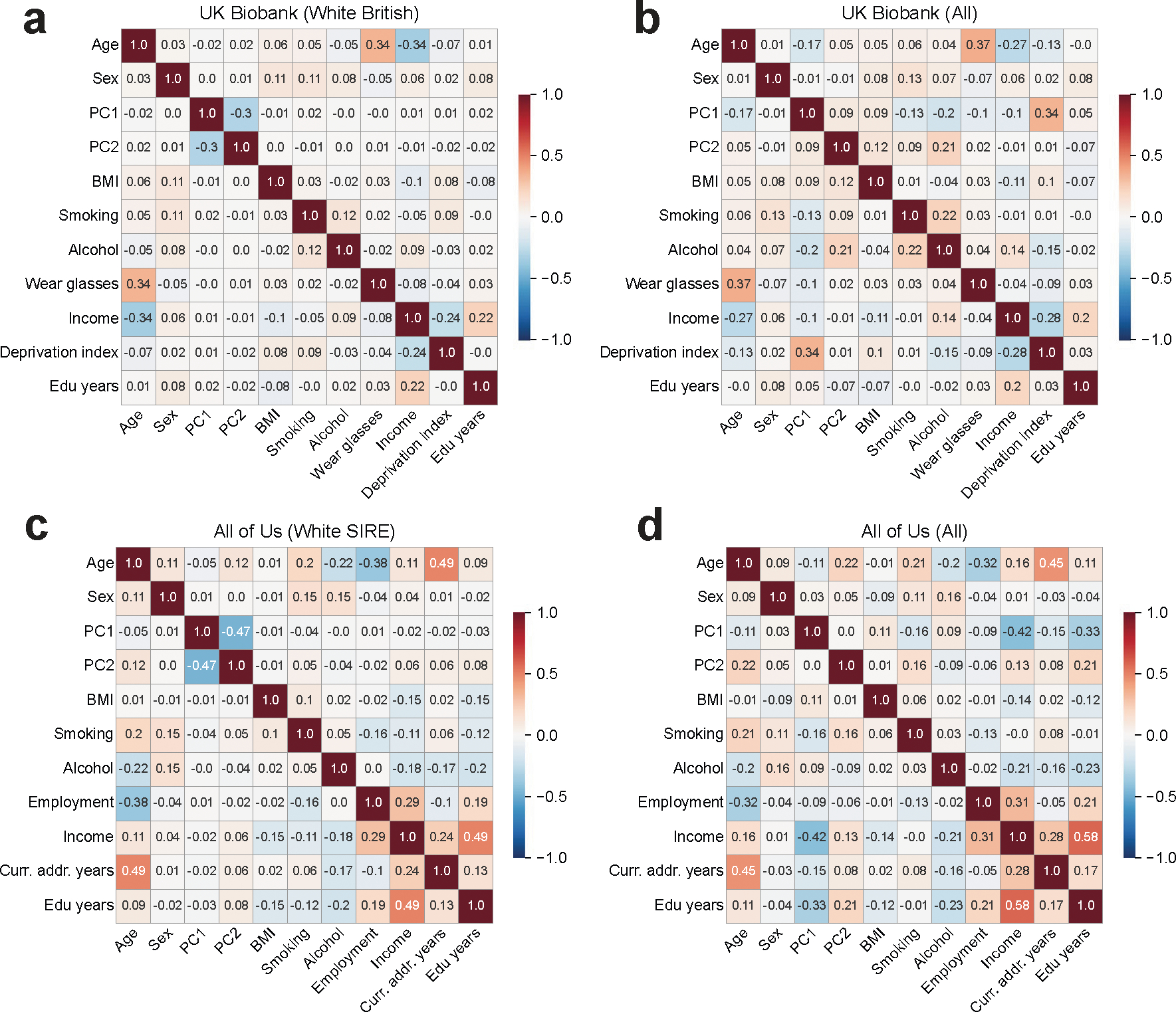
Pearson correlations were calculated separately within individuals annotated with “white British’ in UK Biobank and within individuals with SIRE “white’ in All of Us (a,c) and across all individuals (b,d).

Extended Data Fig. 2 |. Distribution of context variables in UK Biobank.

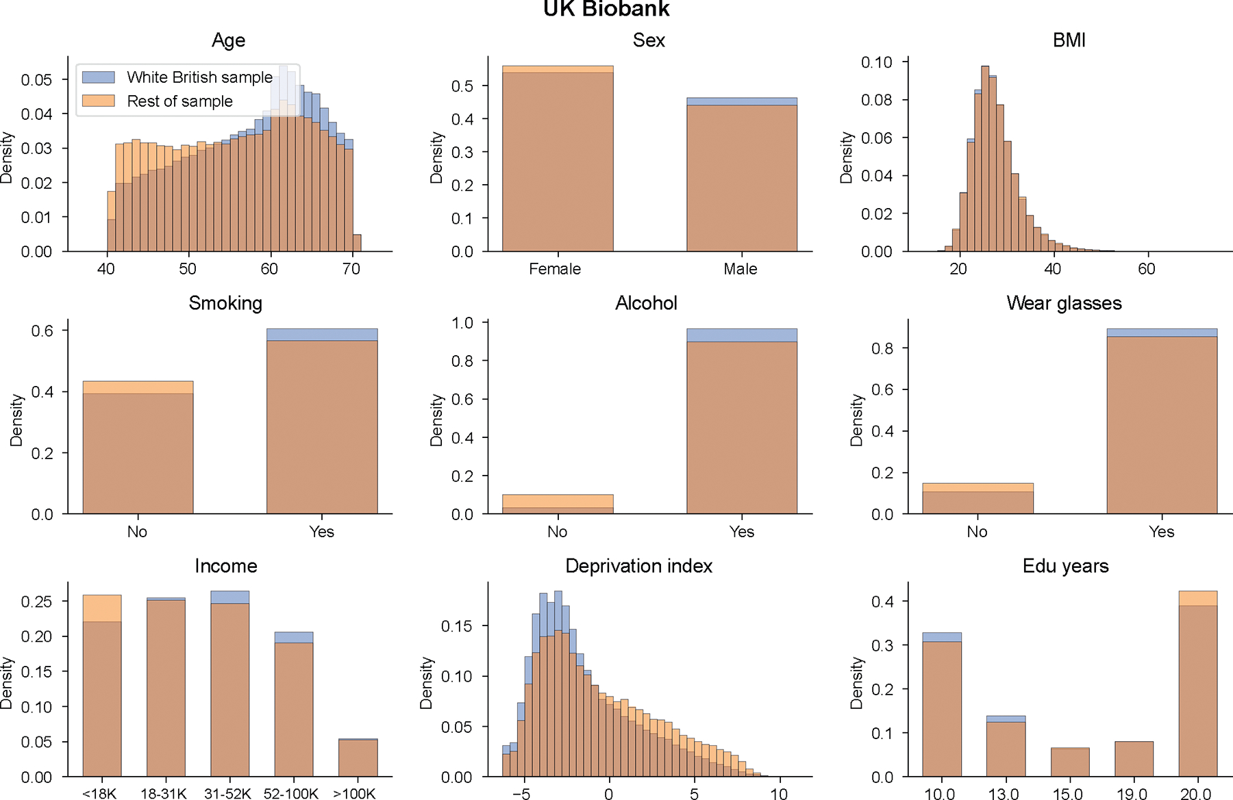
We show context distribution separately for “white British’ individuals and rest of individuals in UK Biobank.

Extended Data Fig. 3 |. Distribution of context variables in All of Us.

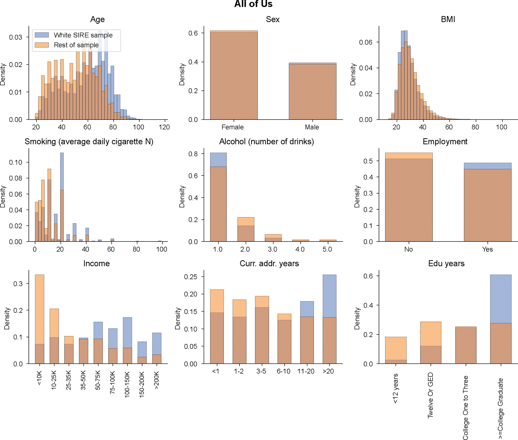
We show context distribution separately for “white SIRE’ individuals and rest of individuals in All of Us.

Extended Data Fig. 4 |. ${\mathrm{R}}^2$ between covariate-adjusted height and PGS across education and income levels in All of Us.

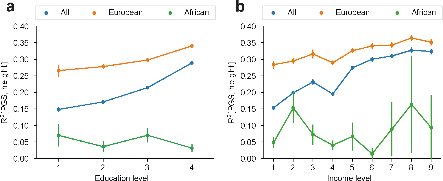
${\mathrm{R}}^2$ were calculated across all individuals, and within individuals of European and African genetic ancestry (with estimated admixture proportion of the corresponding ancestry > 90%), across education levels (a) and income levels (b). Error bars denote mean values +/− standard deviation of ${\mathrm{R}}^2$ across 30 bootstrap samples.

Extended Data Fig. 5 |. Quantitative trait simulations with gene-context interactions.

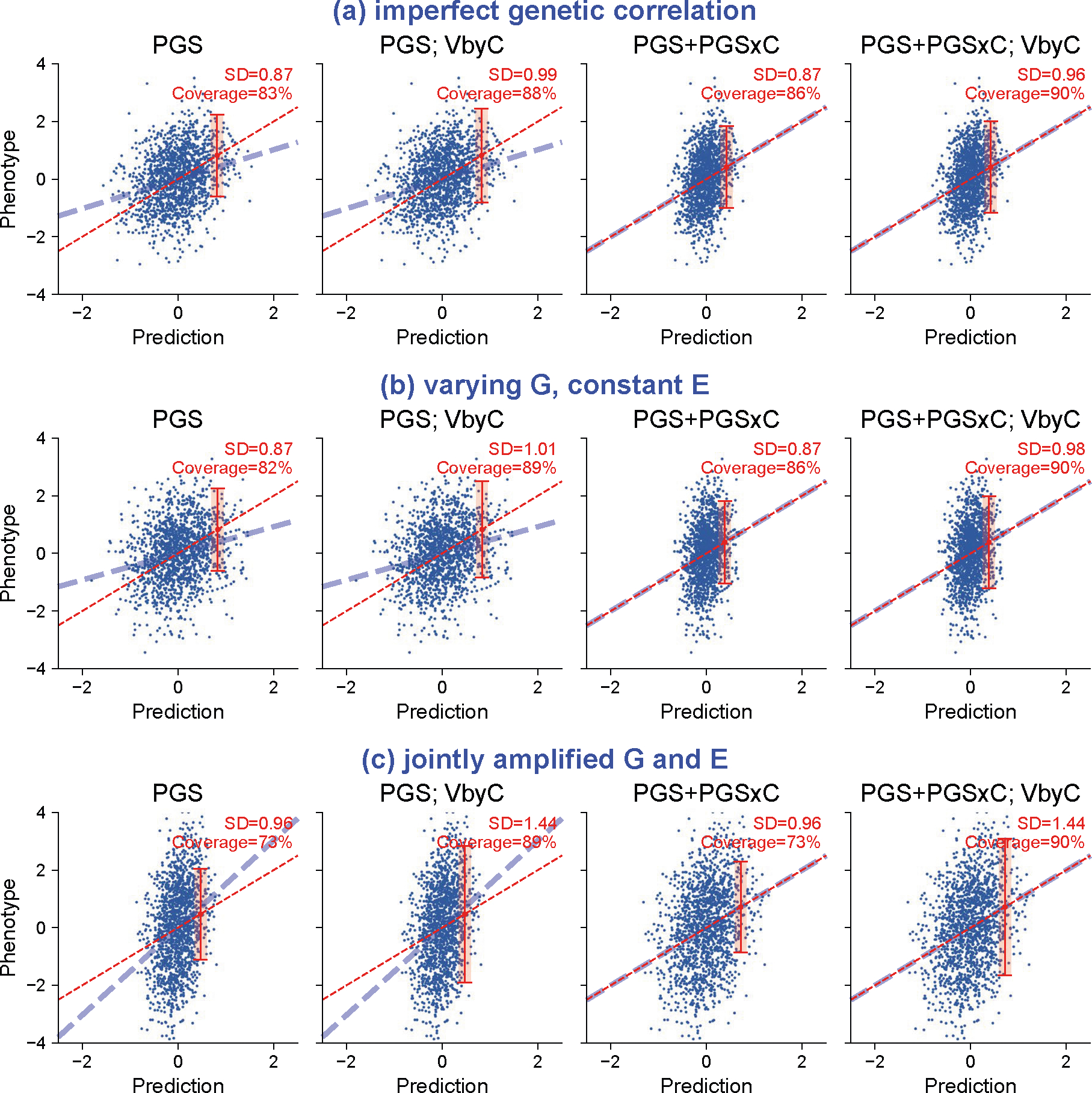
We simulated three scenarios of gene-context interactions for quantitative traits and evaluated calibration of prediction intervals. These scenarios include (a) imperfect genetic correlation: Var[G] = 0.5, Var[E] = 0.5 in both contexts; genetic correlation=0.5 across contexts. (b) varying heritability: Var[G] = 0.5, Var[E] = 0.5 in context 1 and Var[G] = 0.1, Var[E] = 0.9 in context 2; genetic correlation=1. (c) joint amplified G and E: Var[G] = 0.25, Var[E] = 0.75 in context 1 and Var[G] = 0.25*1.5, Var[E] = 0.75*1.5; genetic correlation=1. Across three scenarios, PGS weights derived in the first context were applied to individuals in both contexts. We show results for individuals in context 2 using four modeling approaches. “PGS’: PGS and prediction variance calculated with individuals from context 1 were applied to individuals in context 2; “PGS; VbyC’: fit y ~ N(PGS, VbyC); “PGS+PGSxC’: fit y ~ N(PGS + PGSxC, prediction variance derived in context 1); “PGS+PGSxC; VbyC’: fit y ~ N(PGS + PGSxC, VbyC). Blue dashed line denotes the best fit to data; red dashed line denotes model predictions; red error bar denotes the prediction interval for an individual at top 5% quantile of PGS. Prediction interval coverage was evaluated within data in top PGS decile. We note these three simulation scenarios did not cover all possible modes of gene-context interactions: these models assume gene-context interactions act similarly across all causal variants, and they model gene-context interactions using PGSxC and VbyC.

Extended Data Fig. 6 |. Disease trait simulations with gene-context interactions.

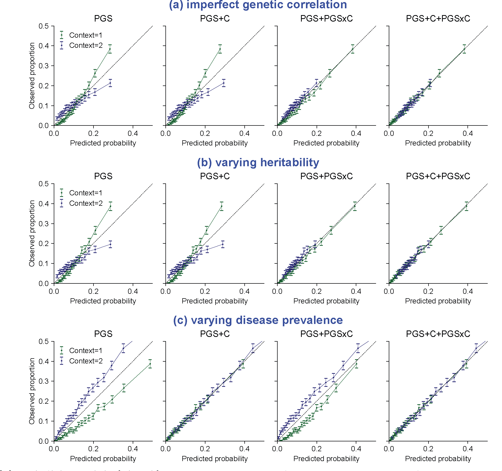
We simulated three scenarios of gene-context interactions for disease traits using a liability threshold model and evaluated calibration of probability prediction. These scenarios include: (a) imperfect genetic correlation: Var[G] = 0.5, Var[E] = 0.5, disease prevalence = 10% in both contexts; genetic correlation=0.5 across two contexts. (b) varying heritability: Var[G] = 0.5, Var[E] = 0.5 in context 1 and Var[G] = 0.1, Var[E] = 0.9 in context 2, disease prevalence=10% in both contexts; genetic correlation=1 across two contexts. (c) varying disease prevalence: Var[G] = 0.5, Var[E] = 0.5 in both contexts; disease prevalence = 10%/20% in context 1/2. Across three scenarios, PGS weights derived in the first context were applied to individuals in both contexts. We fit four models using different sets of predictors in logistic regression across individuals in two contexts (probit regression led to similar results): “PGS’: fit y ~ PGS; “PGS + C’: fit y ~ PGS + Context; “PGS+PGSxC’: fit y ~ PGS + PGSxContext; “PGS+PGSxC+C’: fit y ~ PGS + PGSxContext + Context. Error bars denote observed disease proportions and their 95% confidence intervals for each predicted probability bin (n = 2000 individuals for each error bar).

Extended Data Fig. 7 |. Simulations with varying number of individuals, unmeasured contexts, excessive dummy contexts.

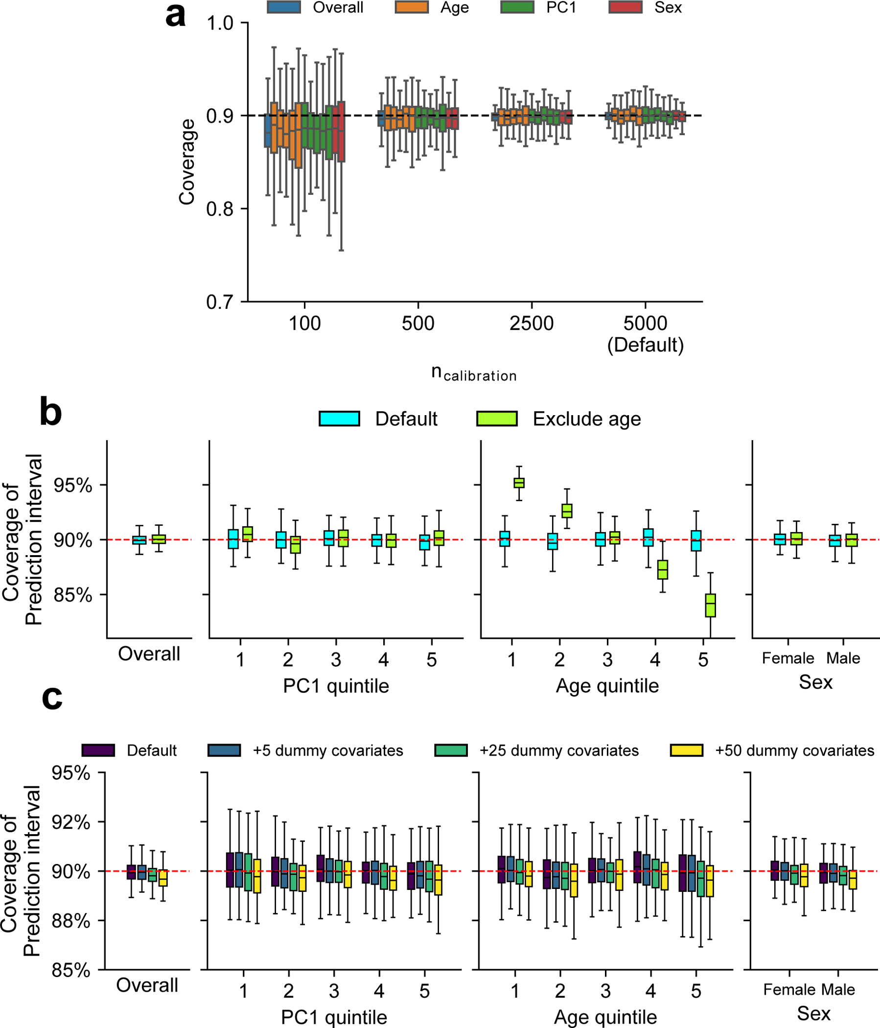
We performed simulations to investigate factors that influence coverage of prediction intervals. We compared coverage in these alternative scenarios with default scenario (marked by ‘Default’ in the figure) where we performed calibration using age, PC1, and sex and 5000 individuals as calibration data (same as Fig. 5). (a) Coverage of prediction intervals with varying number of individuals used in calibration ($N_{\text{cal}}=100,500,2500,5000$). We evaluated the coverage both at the overall level and within each group (groups are denoted by colors) using 5,000 testing individuals. Different box plots with the same color denotes different strata for each context (quintile for age and PC1; male/female for sex). We determined coverages had more downward bias and higher variance when less individuals are used in the calibration. (b) Coverage of prediction intervals when certain context variables were not measured. To simulate unmeasured covariate, we performed calibration using PC1 and sex only (excluding age). And we determined prediction intervals were mis-calibrated along the unmeasured context of age in this scenario. (c) Coverage of prediction intervals when including excessive dummy contexts in calibration. We simulated dummy variables with no effects to phenotype variance (number of dummy covariates $N_{\text{dummy}}=5,25,50$; drawn from N(0,1)) and included them in calibration to investigate the effect of including excessive covariates to prediction coverage. We determined coverages had more downward bias and higher variance when more dummy variables were used in the calibration. For (a-c), each box plot contains results across 100 simulations (each box contains n = 100 points). For box plots, the center corresponds to the median; the box represents the first and third quartiles of the points; the whiskers represent the minimum and maximum points located within 1.5× interquartile ranges from the first and third quartiles, respectively.

Extended Data Fig. 8 |. Standardized effects of PGS, contexts, and PGSxC interaction terms in quantitative trait prediction in All of Us.

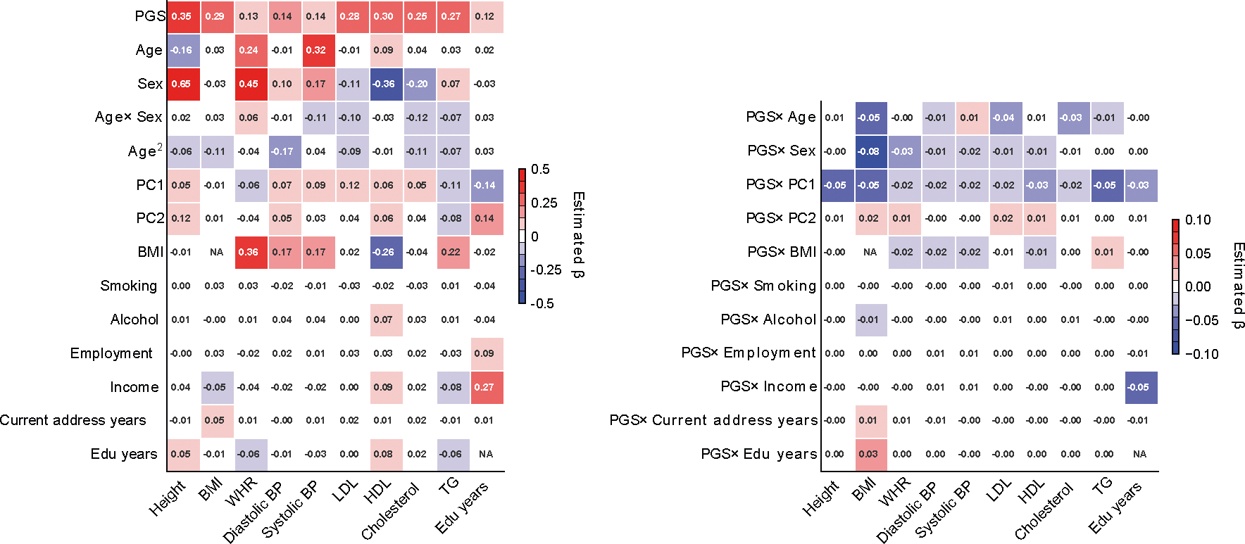
We display standardized effects of all predictors where they are standardized with mean 0 and variance 1 in regression analysis. We note that the left figure containing effects of PGS and contexts has a different color scale than the right figure containing PGSxC interaction terms.

Extended Data Fig. 9 |. Contribution of PGS to inter-individual variation of prediction SDs in All of Us.

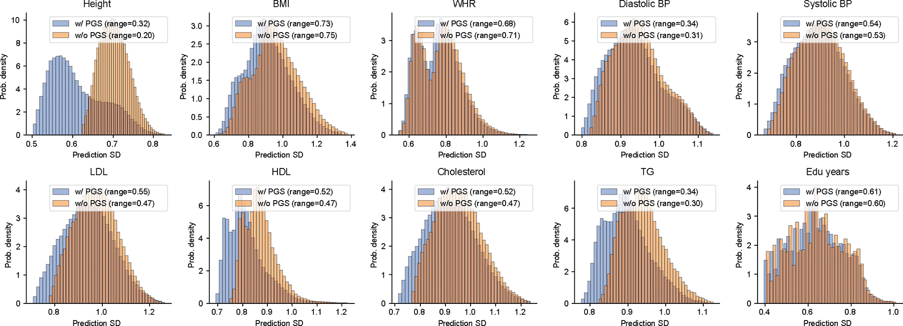
We compared inter-individual variation of prediction SDs in two models: (1) prediction mean as a function of all contexts without PGS; (2) include PGS as part of prediction mean in the baseline model. Prediction SD is modeled as a function of all contexts in both models. By comparing prediction SDs in these two models, we found including PGS substantially impacted inter-individual variation in prediction SD.

Extended Data Fig. 10 |. Standardized effects of PGS, contexts, and PGSxC interaction terms in disease trait prediction in All of Us.

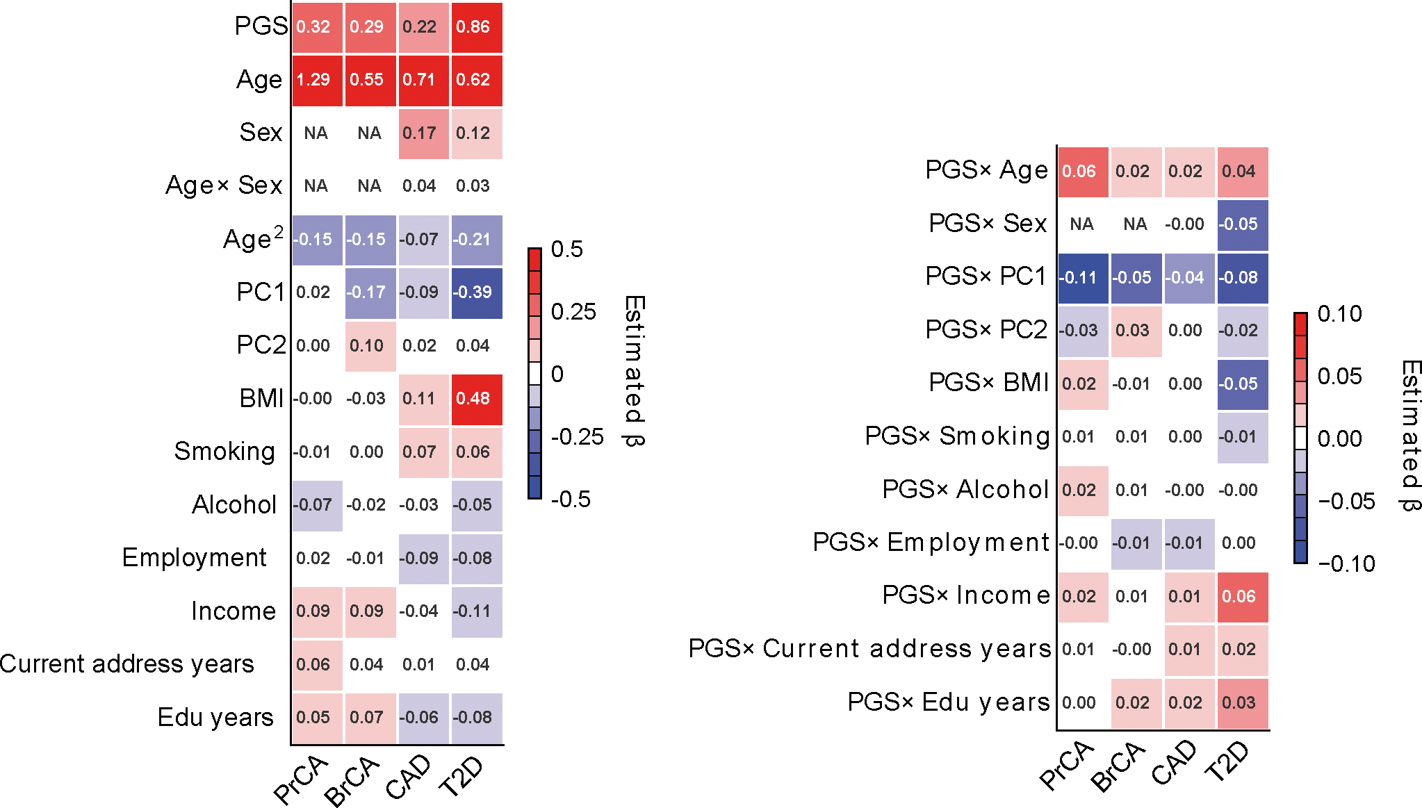
We show standardized effects where all predictor variables are standardized with mean 0 and variance 1 in regression analysis within all individuals. Left figure containing PGS and contexts has different color scale from the right figure containing PGSxC interaction terms.

Data availability

UK Biobank individual-level genotype and phenotype data are available through application at http://www.ukbiobank.ac.uk. All of Us individual-level genotype and phenotype are available through application at https://www.researchallofus.org.

References

- 1.Chatterjee N, Shi J & García-Closas M Developing and evaluating polygenic risk prediction models for stratified disease prevention. Nat. Rev. Genet. 17, 392–406 (2016). [DOI] [PMC free article] [PubMed] [Google Scholar]
- 2.Torkamani A, Wineinger NE & Topol EJ The personal and clinical utility of polygenic risk scores. Nat. Rev. Genet. 19, 581–590 (2018). [DOI] [PubMed] [Google Scholar]
- 3.Li R, Chen Y, Ritchie MD & Moore JH Electronic health records and polygenic risk scores for predicting disease risk. Nat. Rev. Genet. 21, 493–502 (2020). [DOI] [PubMed] [Google Scholar]
- 4.Kullo IJ et al. Polygenic scores in biomedical research. Nat. Rev. Genet. 23, 524–532 (2022). [DOI] [PMC free article] [PubMed] [Google Scholar]
- 5.Martin AR et al. Clinical use of current polygenic risk scores may exacerbate health disparities. Nat. Genet. 51, 584–591 (2019). [DOI] [PMC free article] [PubMed] [Google Scholar]
- 6.Ding Y et al. Large uncertainty in individual polygenic risk score estimation impacts PRS-based risk stratification. Nat. Genet. 54, 30–39 (2022). [DOI] [PMC free article] [PubMed] [Google Scholar]
- 7.Privé F et al. Portability of 245 polygenic scores when derived from the UK Biobank and applied to 9 ancestry groups from the same cohort. Am. J. Hum. Genet. 109, 12–23 (2022). [DOI] [PMC free article] [PubMed] [Google Scholar]
- 8.Weissbrod O et al. Leveraging fine-mapping and multipopulation training data to improve cross-population polygenic risk scores. Nat. Genet. 54, 450–458 (2022). [DOI] [PMC free article] [PubMed] [Google Scholar]
- 9.Ruan Y et al. Improving polygenic prediction in ancestrally diverse populations. Nat. Genet. 54, 573–580 (2022). [DOI] [PMC free article] [PubMed] [Google Scholar]
- 10.Bitarello BD & Mathieson I Polygenic scores for height in admixed populations. G3 10, 4027–4036 (2020). [DOI] [PMC free article] [PubMed] [Google Scholar]
- 11.Mostafavi H et al. Variable prediction accuracy of polygenic scores within an ancestry group. eLife 9, e48376 (2020). [DOI] [PMC free article] [PubMed] [Google Scholar]
- 12.Jiang X, Holmes C & McVean G The impact of age on genetic risk for common diseases. PLoS Genet. 17, e1009723 (2021). [DOI] [PMC free article] [PubMed] [Google Scholar]
- 13.Hui D et al. Quantifying factors that affect polygenic risk score performance across diverse ancestries and age groups for body mass index. Pac. Symp. Biocomput. 28, 437–448 (2023). [PMC free article] [PubMed] [Google Scholar]
- 14.Wray NR et al. Pitfalls of predicting complex traits from SNPs. Nat. Rev. Genet. 14, 507–515 (2013). [DOI] [PMC free article] [PubMed] [Google Scholar]
- 15.Ge T, Chen C-Y, Neale BM, Sabuncu MR & Smoller JW Phenome-wide heritability analysis of the UK Biobank. PLoS Genet. 13, e1006711 (2017). [DOI] [PMC free article] [PubMed] [Google Scholar]
- 16.Zhu C et al. Amplification is the primary mode of gene-by-sex interaction in complex human traits. Cell Genom. 3, 100297 (2023). [DOI] [PMC free article] [PubMed] [Google Scholar]
- 17.Brown BC, Ye CJ, Price AL & Zaitlen N Transethnic genetic-correlation estimates from summary statistics. Am. J. Hum. Genet. 99, 76–88 (2016). [DOI] [PMC free article] [PubMed] [Google Scholar]
- 18.Shi H et al. Population-specific causal disease effect sizes in functionally important regions impacted by selection. Nat. Commun. 12, 1098 (2021). [DOI] [PMC free article] [PubMed] [Google Scholar]
- 19.Patel RA et al. Genetic interactions drive heterogeneity in causal variant effect sizes for gene expression and complex traits. Am. J. Hum. Genet. 109, 1286–1297 (2022). [DOI] [PMC free article] [PubMed] [Google Scholar]
- 20.Weine E, Smith SP, Knowlton RK & Harpak A Tradeoffs in modeling context dependency in complex trait genetics. Preprint at bioRxiv 10.1101/2023.06.21.545998 (2023). [DOI] [Google Scholar]
- 21.Wang Y et al. Theoretical and empirical quantification of the accuracy of polygenic scores in ancestry divergent populations. Nat. Commun. 11, 3865 (2020). [DOI] [PMC free article] [PubMed] [Google Scholar]
- 22.Lambert SA, Abraham G & Inouye M Towards clinical utility of polygenic risk scores. Hum. Mol. Genet. 28, R133–R142 (2019). [DOI] [PubMed] [Google Scholar]
- 23.Ding Y et al. Polygenic scoring accuracy varies across the genetic ancestry continuum. Nature 618, 774–781 (2023). [DOI] [PMC free article] [PubMed] [Google Scholar]
- 24.Johnson R et al. Leveraging genomic diversity for discovery in an electronic health record linked biobank: the UCLA ATLAS Community Health Initiative. Genome Med. 14, 104 (2022). [DOI] [PMC free article] [PubMed] [Google Scholar]
- 25.Wiley LK et al. Building a vertically integrated genomic learning health system: the biobank at the Colorado Center for Personalized Medicine. Am. J. Hum. Genet. 111, 11–23 (2024). [DOI] [PMC free article] [PubMed] [Google Scholar]
- 26.Belbin GM et al. Toward a fine-scale population health monitoring system. Cell 184, 2068–2083.e11 (2021). [DOI] [PubMed] [Google Scholar]
- 27.Abul-Husn NS & Kenny EE Personalized medicine and the power of electronic health records. Cell 177, 58–69 (2019). [DOI] [PMC free article] [PubMed] [Google Scholar]
- 28.Bycroft C et al. The UK Biobank resource with deep phenotyping and genomic data. Nature 562, 203–209 (2018). [DOI] [PMC free article] [PubMed] [Google Scholar]
- 29.The All of Us Research Program Genomics Investigators et al. Genomic data in the All of Us Research Program. Nature 627, 340–346 (2024). [DOI] [PMC free article] [PubMed] [Google Scholar]
- 30.Wand H et al. Improving reporting standards for polygenic scores in risk prediction studies. Nature 591, 211–219 (2021). [DOI] [PMC free article] [PubMed] [Google Scholar]
- 31.Wei J et al. Calibration of polygenic risk scores is required prior to clinical implementation: results of three common cancers in UKB. J. Med. Genet. 59, 243–247 (2022). [DOI] [PubMed] [Google Scholar]
- 32.van Houwelingen HC Validation, calibration, revision and combination of prognostic survival models. Stat. Med. 19, 3401–3415 (2000). [DOI] [PubMed] [Google Scholar]
- 33.Van Calster B et al. Calibration: the Achilles heel of predictive analytics. BMC Med. 17, 230 (2019). [DOI] [PMC free article] [PubMed] [Google Scholar]
- 34.Sun J et al. Translating polygenic risk scores for clinical use by estimating the confidence bounds of risk prediction. Nat. Commun. 12, 5276 (2021). [DOI] [PMC free article] [PubMed] [Google Scholar]
- 35.Smyth GK Generalized linear models with varying dispersion. J. R. Stat. Soc 51, 47–60 (1989). [Google Scholar]
- 36.Koenker R Quantile Regression (Cambridge Univ. Press, 2005). [Google Scholar]
- 37.Rigby RA & Stasinopoulos DM Generalized additive models for location, scale and shape. J. R. Stat. Soc. Ser. C 54, 507–554 (2005). [Google Scholar]
- 38.Romano Y, Patterson E & Candès EJ Conformalized quantile regression. Advances in Neural Information Processing Systems 32 (2019). [Google Scholar]
- 39.Gneiting T & Katzfuss M Probabilistic forecasting. Annu. Rev. Stat. Appl. 1, 125–151 (2014). [Google Scholar]
- 40.Yang J et al. FTO genotype is associated with phenotypic variability of body mass index. Nature 490, 267–272 (2012). [DOI] [PMC free article] [PubMed] [Google Scholar]
- 41.Young AI, Wauthier FL & Donnelly P Identifying loci affecting trait variability and detecting interactions in genome-wide association studies. Nat. Genet. 50, 1608–1614 (2018). [DOI] [PubMed] [Google Scholar]
- 42.Miao J et al. A quantile integral linear model to quantify genetic effects on phenotypic variability. Proc. Natl Acad. Sci. USA 119, e2212959119 (2022). [DOI] [PMC free article] [PubMed] [Google Scholar]
- 43.Schoeler T et al. Participation bias in the UK Biobank distorts genetic associations and downstream analyses. Nat. Hum. Behav. 10.1038/s41562-023-01579-9 (2023). [DOI] [PMC free article] [PubMed] [Google Scholar]
- 44.Selzam S et al. Comparing within- and between-family polygenic score prediction. Am. J. Hum. Genet. 105, 351–363 (2019). [DOI] [PMC free article] [PubMed] [Google Scholar]
- 45.Okbay A et al. Polygenic prediction of educational attainment within and between families from genome-wide association analyses in 3 million individuals. Nat. Genet. 54, 437–449 (2022). [DOI] [PMC free article] [PubMed] [Google Scholar]
- 46.Yengo L et al. A saturated map of common genetic variants associated with human height. Nature 610, 704–712 (2022). [DOI] [PMC free article] [PubMed] [Google Scholar]
- 47.Graham SE et al. The power of genetic diversity in genome-wide association studies of lipids. Nature 600, 675–679 (2021). [DOI] [PMC free article] [PubMed] [Google Scholar]
- 48.Lambert SA et al. The polygenic score catalog as an open database for reproducibility and systematic evaluation. Nat. Genet. 53, 420–425 (2021). [DOI] [PMC free article] [PubMed] [Google Scholar]
- 49.Durvasula A & Price AL Distinct explanations underlie gene–environment interactions in the UK Biobank. Preprint at medRxiv 10.1101/2023.09.22.23295969 (2023). [DOI] [Google Scholar]
- 50.Mahajan A et al. Fine-mapping type 2 diabetes loci to single-variant resolution using high-density imputation and islet-specific epigenome maps. Nat. Genet. 50, 1505–1513 (2018). [DOI] [PMC free article] [PubMed] [Google Scholar]
- 51.Patel AP et al. A multi-ancestry polygenic risk score improves risk prediction for coronary artery disease. Nat. Med. 29, 1793–1803 (2023). [DOI] [PMC free article] [PubMed] [Google Scholar]
- 52.Schumacher FR et al. Association analyses of more than 140,000 men identify 63 new prostate cancer susceptibility loci. Nat. Genet. 50, 928–936 (2018). [DOI] [PMC free article] [PubMed] [Google Scholar]
- 53.Zhang H et al. Genome-wide association study identifies 32 novel breast cancer susceptibility loci from overall and subtype-specific analyses. Nat. Genet. 52, 572–581 (2020). [DOI] [PMC free article] [PubMed] [Google Scholar]
- 54.Martin AR et al. Human demographic history impacts genetic risk prediction across diverse populations. Am. J. Hum. Genet. 107, 788–789 (2020). [DOI] [PMC free article] [PubMed] [Google Scholar]
- 55.Kachuri L et al. Genetically adjusted PSA levels for prostate cancer screening. Nat. Med. 29, 1412–1423 (2023). [DOI] [PMC free article] [PubMed] [Google Scholar]
- 56.Smyth GK An efficient algorithm for REML in heteroscedastic regression. J. Comput. Graph. Stat. 11, 836–847 (2002). [Google Scholar]
- 57.Giner G & Smyth GK statmod: probability calculations for the inverse Gaussian distribution. The R Journal 8, 339–351 (2016). [Google Scholar]
- 58.Yousefi PD et al. DNA methylation-based predictors of health: applications and statistical considerations. Nat. Rev. Genet. 23, 369–383 (2022). [DOI] [PubMed] [Google Scholar]
- 59.The International HapMap 3 Consortium. Integrating common and rare genetic variation in diverse human populations. Nature 467, 52–58 (2010). [DOI] [PMC free article] [PubMed] [Google Scholar]
- 60.Privé F, Arbel J & Vilhjálmsson BJ LDpred2: better, faster, stronger. Bioinformatics 36, 5424–5431 (2020). [DOI] [PMC free article] [PubMed] [Google Scholar]
- 61.Szczerbinski L et al. Algorithms for the identification of prevalent diabetes in the All of Us Research Program validated using polygenic scores—a new resource for diabetes precision medicine. Preprint at bioRxiv 10.1101/2023.09.05.23295061 (2023). [DOI] [Google Scholar]
- 62.Hou K KangchengHou/calpred. Zenodo; 10.5281/zenodo.10962189 (2024) [DOI] [Google Scholar]
- 63.Hou K KangchengHou/calpred-manuscript. Zenodo; 10.5281/zenodo.11094535 (2024) [DOI] [Google Scholar]
Associated Data
This section collects any data citations, data availability statements, or supplementary materials included in this article.
Supplementary Materials
Data Availability Statement