Abstract
Background
Accurate delineation of knee bone boundaries is crucial for computer-aided diagnosis (CAD) and effective treatment planning in knee diseases. Current methods often struggle with precise segmentation due to the knee joint’s complexity, which includes intricate bone structures and overlapping soft tissues. These challenges are further complicated by variations in patient anatomy and image quality, highlighting the need for improved techniques. This paper presents a novel semi-automatic segmentation method for extracting knee bones from sequential computed tomography (CT) images.
Methods
Our approach integrates the fuzzy C-means (FCM) algorithm with an adaptive region-based active contour model (ACM). Initially, the FCM algorithm assigns membership degrees to each voxel, distinguishing bone regions from surrounding soft tissues based on their likelihood of belonging to specific bone regions. Subsequently, the adaptive region-based ACM utilizes these membership degrees to guide the contour evolution and refine segmentation boundaries. To ensure clinical applicability, we further enhance our method using the marching cubes algorithm to reconstruct a three-dimensional (3D) model. We evaluated the method on six randomly selected knee joints.
Results
We evaluated the method using quantitative metrics such as the Dice coefficient, sensitivity, specificity, and geometrical assessment. Our method achieved high Dice scores for the femur (98.95%), tibia (98.10%), and patella (97.14%), demonstrating superior accuracy. Remarkably low root mean square distance (RSD) values were obtained for the tibia and femur (0.5±0.14 mm) and patella (0.6±0.13 mm), indicating precise segmentation.
Conclusions
The proposed method offers significant advancements in CAD systems for knee pathologies. Our approach demonstrates superior performance in achieving precise and accurate segmentation of knee bones, providing valuable insights for anatomical analysis, surgical planning, and patient-specific prostheses.
Keywords: Knee bone segmentation, fuzzy-C means (FCM), adaptive region based active contour model (adaptive region based ACM), three-dimensional reconstruction (3D reconstruction), marching cubes algorithm
Introduction
Musculoskeletal disorders are a significant concern in healthcare, driving the need for advanced computer-aided diagnosis (CAD) systems to efficiently detect knee disorders (1). These systems not only reduce the workload for medical professionals but also minimize the inherent variability in manual assessments. Accurate and precise bone segmentation from Computed tomography (CT) images is pivotal for thorough evaluation, staging, and treatment planning. Traditionally, experts have relied on manual segmentation methods, which involve labor-intensive annotation or region of interest (ROI) marking on knee scans. However, these manual approaches are time-consuming, laborious, and subject to human variability (2).
Automating the knee image segmentation process presents a promising solution to the challenges of manual segmentation. In recent years, there has been a remarkable advancement in automated segmentation methods from classical image processing techniques to sophisticated deep learning-based approaches. Despite these advancements, automating knee image segmentation remains challenging due to issues like low image contrast, complex knee structures, and intensity variations within the ROI (3).
Knee arthroplasty has significantly evolved since its inception in the 1960s, when early efforts laid the groundwork for modern joint replacement procedures (4). Initially, techniques focused primarily on alleviating pain and restoring basic joint function but were limited by the materials and surgical methods available at the time. Over the decades, advancements in biomaterials, prosthetic design, and surgical techniques have significantly improved knee arthroplasty outcomes (5).
In the contemporary clinical landscape, the primary indications for knee arthroplasty include end-stage osteoarthritis, rheumatoid arthritis, and post-traumatic arthritis. These conditions lead to severe joint pain, deformity, and functional impairment, profoundly impacting patients’ quality of life. Osteoarthritis, in particular, is the most common reason for knee replacement, characterized by the degeneration of cartilage and underlying bone, resulting in pain and stiffness (6).
Modern knee arthroplasty procedures involve the precise removal of damaged cartilage and bone, followed by the placement of highly durable artificial implants (7). These implants are designed to replicate the natural movement and function of the knee joint, thereby restoring mobility and reducing pain. The procedure typically includes steps such as preoperative planning using imaging, bone resection, implant fitting, and postoperative rehabilitation (8). Recent advancements have focused on developing patient-specific instrumentation (PSI) and computer-assisted surgery (CAS), which enhance the precision of implant placement and alignment (9). Accurate alignment is crucial for the longevity of the implant and overall success of the procedure, as misalignment can lead to increased wear, implant failure, and the need for revision surgery (10).
Knee replacement surgery has significantly advanced, with personalized procedures tailored to each patient’s unique anatomy. This process begins with a CT scan of the patient’s knee joint, from which a precise three-dimensional (3D) model of the knee anatomy is generated. This model serves as the foundation for subsequent surgical planning. The accurate and automated segmentation of knee bones from CT images is crucial in clinical settings, offering streamlined workflows and cost-effective solutions (11). The demand for effective knee joint treatments, including total knee arthroplasty (TKA), has significantly increased. In 2019, 374,833 TKA surgeries were performed in China (12). Furthermore, projections indicate that TKA surgeries will escalate to 1.26 million by 2030 in the United States (13).
CT imaging provides high-definition images with an exceptional signal-to-noise ratio, making it a powerful non-invasive modality (14). CT imaging offers superior tissue differentiation capabilities, providing enhanced contrast for visualizing bone structures. Compared to magnetic resonance imaging (MRI), CT images deliver higher spatial resolution, ensuring finer detail and greater accuracy in bone imaging (15).
Previous studies on automatic knee bone segmentation have primarily focused on magnetic resonance (MR) data, utilizing voxel-based (16) or block-wise classification techniques (17) that incorporate texture features and intensity distribution. However, these methods have struggled to effectively address the significant intensity and texture variations present in both CT and MR images. To enhance segmentation robustness, many studies have used statistical shape models (SSM) (18-20) as prior knowledge to guide the segmentation process. Despite their potential, these methods face challenges in achieving fast and accurate model initialization and adaptation. Graph-based algorithms (21) have been extensively utilized for various vision tasks, including bone segmentation (22-24). However, the accuracy of such algorithms usually depends on seed points often manually provided. Moreover, bones are often segmented individually rather than jointly, leading to suboptimal segmentation results, particularly in regions where bones are in close proximity or touching, potentially causing overlapping segmentations.
Deep learning approaches have gained significant recognition due to their outstanding results in image segmentation (25). However, these approaches often require large annotated datasets for training (26), which can be problematic in applications where only limited images are available. Recent advancements, including transfer learning (27), unsupervised domain adaptation (28) and zero-shot learning (29), have been introduced to mitigate the challenge of limited training data. Traditional methods based on unsupervised learning offer distinct advantages, including providing interpretable and explainable results and requiring less computational power compared to deep learning methods. Multiple methods have been presented in recent studies For instance, Almajalid et al. (30) presented a fully automatic detection and segmentation method for knee bone based on modified U-Net models, achieving Dice indices of 97% for the femur, 96% for the tibia, and 92% for the patella. Ambellan et al. (18) introduced a robust segmentation technique using a 3D SSM combined with convolutional neural networks (CNNs) to segment bone and cartilage. Hohlmann et al. (31) proposed a method using SSM for 3D reconstruction from ultrasound (US) images, enhancing accuracy and reliability in generating detailed 3D models. Liu et al. (32) introduced a knee joint segmentation method using adversarial networks. du Toit et al. (33) presented a deep learning architecture using a modified 2D U-Net network for segmenting the femoral articular cartilage in 3D US knee images. Hall et al. (34) proposed a watershed algorithm to segment tibial cartilage in CT images. Additionally Liu et al. (35) performed segmentation of femur, tibia, and cartilages using deep CNNs and a 3D deformable approach. Their segmentation pipeline was based on a 10-layers SegNet using 2D knee images.
Liu et al. (36) introduced a novel 3D U-Net neural network approach, leveraging prior knowledge, for segmenting knee cartilage in MRI images. Li et al. (37) proposed a deep learning algorithm based on plain radiographs for detecting and classifying knee osteoarthritis, achieving an accuracy of 96%. Mahum et al. (38) developed a CNN-based method for classifying knee osteoarthritis, achieving a classification accuracy of up to 97%. Norman et al. (39) applied an end-to-end automatic segmentation technique without any extensive pipeline for image registration. Chadoulos et al. (40) utilized a multi-atlas-based model to segment cartilage, attaining Dice similarity coefficient (DSC) values of 88% and 85% for femur and tibial cartilage, respectively. Gandhamal et al. (41) presented a hierarchical level-set-based method for segmenting knee bones, yielding good results but struggling with small or separated bone regions. Cheng et al. (42) developed a simplified CNN-based architecture, termed a holistically nested network (HNN), for segmenting the femur and tibial bone. Chen et al. (43) presented a YOLOV2-based detection mechanism for knee joints, utilizing various transfer learning-based pre-trained models. Peng et al. (44) introduced a sparse annotation-based framework for accurate knee cartilage and bone segmentation in 3D MR images. Chadoulos et al. (45) proposed a multi-view knee cartilage segmentation method from MR images, achieving an accuracy of up to 92%. Deschamps et al. (46) presented an innovative approach based on hierarchal clustering to detect joint coupling patterns in lower limbs. Rahman et al. (47) introduced a novel approach for bone surface segmentation using a graph convolutional network (GCN), focusing on enhancing network connectivity by incorporating graph convolutions.
Despite significant advancements in automated segmentation methods, precise segmentation of knee bones remains challenging due to the complex anatomy of the knee joint, which features intricate bone formations and overlapping soft tissues. Many existing methods are either computationally intensive or require extensive annotated datasets for training, which may not be feasible in all clinical settings. Our study aims to address these challenges by developing a robust segmentation method that enhances anatomical fidelity, minimizes segmentation errors, and adapts to variations in CT image quality and patient anatomy. This approach ensures high accuracy and reliability in segmenting knee bones from CT images while maintaining efficiency.
This paper introduces a novel medical image segmentation pipeline designed to accurately segment knee bones from CT images. The methodology involves a two-step process: an initial pre-segmentation step followed by a segmentation refinement step. Initially, the ROI is extracted using the contour extraction method based on Canny edge detection. Subsequently, a refinement step is applied to the pre-segmented data using the fuzzy C-means (FCM) clustering method, which incorporates spatial constraints to improve segmentation outcomes. The segmentation is further refined using an adaptive region-based active contour model (ACM), which utilizes specialized region descriptors to guide the contour’s movement and ensure precise identification of the ROI boundaries. The detailed flowchart of the manuscript is illustrated in Figure 1.
Figure 1.
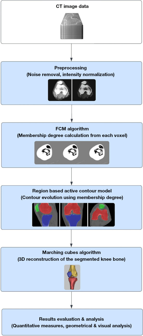
Flowchart of the proposed methodology. CT, computed tomography; FCM, fuzzy C-means.
The manuscript is organized into the following sections: section “Methods” provides a detailed description and working of our proposed methodology. Section “Results” presents the segmentation results and discussion, highlighting the performance of our method. Lastly, section “Discussion and Conclusions” presents the conclusion.
Methods
The study was conducted in accordance with the Declaration of Helsinki (as revised in 2013) and informed consent was obtained from all volunteers who participated in the study. Ethical approval for this study was waived by the ethics committee of Second Affiliated Hospital of Dalian Medical University.
Dataset preparation
In our study, we utilized CT images from twenty patients, comprising fifteen males and five females. The CT scans were acquired using a standardized protocol with a slice thickness and interval of 0.5 mm, a window width of 2,000 Hounsfield units (HU), and a window level of 500 HU. These images were in DICOM format, with a resolution of 512×512 pixel and a spatial resolution of 0.5 mm per pixel. Each dataset consisted of 100 to 300 slices taken in the axial plane. The CT datasets were collected from the Second Affiliated Hospital of Dalian Medical University. In compliance with ethical considerations, all patient-specific information was anonymized to maintain privacy.
Dataset preprocessing
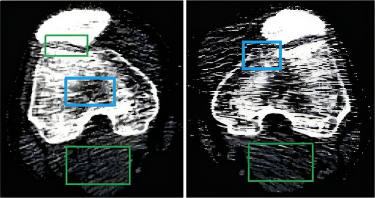
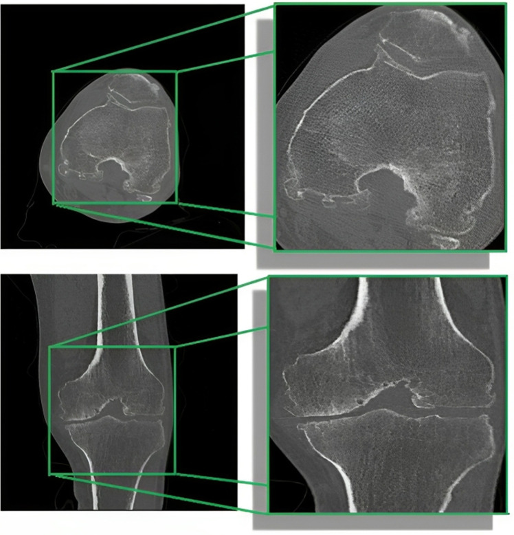
The objective of pre-processing is to enhance the image quality, as CT scanner-acquired data frequently contains a variety of artifacts, including noise and distortion, which can adversely affect segmentation accuracy (48). These complexities in CT images are illustrated in Figure 2. To improve the quality of knee bone CT scans and reduce noise artifacts, we applied a thresholding technique, setting pixel intensities outside the bone intensity range of 100 to 1,500 HU to zero. This step ensures that only bone tissues are retained, eliminating other structures and artifacts. Initially, we performed image cropping to remove extraneous background and soft tissue pixels, simplifying the dataset and reducing computational complexity. This step involved defining the boundaries based on consistent anatomical landmarks, specifically the distal femur, proximal tibia, and patella, to cover the entire knee joint area. The cropping ensured the inclusion of all relevant bone structures while accommodating anatomical differences and variations in patient positioning. Figure 3 provides a visual representation of the cropped region.
Figure 2.
CT images showing complexities such as regions of soft tissues, noises, and intensity inhomogeneity across different slices. The green marked boxes identify areas corresponding to soft tissues and noises, while the blue boxes highlight regions of intensity inhomogeneity. CT, computed tomography.
Figure 3.
Cropping of knee CT image to eliminate extraneous background details and extract relevant bone structures. CT, computed tomography.
The segmentation technique presented in this work was implemented using Python programming language, specifically on the PyCharm platform. Key libraries for image processing and visualization included Open-Source Computer Vision Library (OpenCV) and Visualization Toolkit (VTK).
Contour detection
A contour extraction method based on Canny edge detection is employed to extract the knee joint region from DICOM images. This method effectively locates and extracts the pixels corresponding to the knee joint’s ROI. The Canny edge detection algorithm is optimal for detecting edges in images, adhering to well-defined criteria: maximizing edge detection while minimizing the error rate, accurately localizing edges close to the true edges, and ensuring single-edge detection for minimal responses. This is achieved through the application of a Gaussian filter, as shown in Eq. [1]:
| [1] |
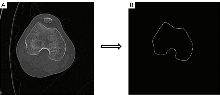
Here, σ represents the Gaussian standard deviation, set at 1.4, to smooth the image and enhance edge detection. The low and high thresholds for edge detection were set at 0.1 and 0.4 times the maximum gradient, respectively. Additionally, adaptive thresholding techniques were implemented to dynamically adjust threshold values based on local image characteristics. The selection of the optimal filter is based on two key factors: the σ value, which controls the degree of smoothing, and the filter size, which determines the sensitivity to noise. Empirical experimentation and literature review guided the selection of these parameters, conclusively determining that a Gaussian standard deviation (σ) of 1.4 and a filter size of (3×3) produced optimal results. As the filter size increases, sensitivity to noise decreases, leading to the preservation of more accurate edge information. The canny algorithm is then applied to detect edges, as shown in Eq. [2] and Eq. [3]. The results are shown in Figure 4.
Figure 4.
Outer contour extraction of the knee CT image. (A) Knee CT image showing the original data. (B) Outer contour extraction using Canny edge detection with a σ value of 1.4). CT, computed tomography.
| [2] |
| [3] |
Here and represents the mean magnitudes of the horizontal and vertical gradient, respectively, while denoting the count of connected pixels associated with each pixel position.
FCM segmentation
FCM clustering is renowned for its efficiency and versatility, making it a widely adopted technique in diverse fields (49). FCM, an unsupervised clustering method, classifies image voxels into distinct clusters based on their similarity within a multidimensional feature space (50). In our implementation, FCM clustering is integrated with pre-extracted knee joint contours to incorporate additional spatial context into the segmentation process. Each voxel is represented as a feature vector with intensity values, and FCM clusters these voxels based on their inherent similarities within the knee joint region. This integration not only simplifies the segmentation process but also ensures smoother results, particularly in regions with intricate anatomical features.
To address the sensitivity of FCM to noise and image artifacts, we introduced a spatial penalty term into the objective function. This penalty discourages the assignment of spatially distant voxels to the same cluster unless their intensity values are similar. By incorporating this spatial penalty, our method maintains spatial coherence and reduces the algorithm’s sensitivity to noise and artifacts. Specifically, the spatial penalty mitigates the effects of Gaussian noise by favoring spatially adjacent voxels. Experimental results demonstrate that our method remains robust across various levels of Gaussian noise, maintaining accurate segmentation performance even with a standard deviation of up to 20. The enhanced optimization objective function, denoted as E, is defined as:
| [4] |
Here, n represents the voxel count, c represents the total number of clusters, m denotes the fuzziness parameter, represents the membership degree of the voxel in the cluster, corresponds to the feature vector of the voxel, and represents the centroid of the cluster. The term quantifies the dissimilarity between the feature vector of the voxel and the centroid of the cluster. The term represents the spatial distance penalty between voxel i and cluster centroid ϳ, and λ is a weight parameter balancing the intensity and spatial terms. The membership degrees are updated using the Eq. [5]:
| [5] |
where denotes the Euclidean distance between the feature vector of the voxel and the centroid of the cluster. This updated equation calculates the membership degree based on the relative distances between the voxel and the cluster centroids. The fuzziness parameter m controls the degree of fuzziness of the clusters, with higher values resulting in softer clusters. The centroids were recalculated based on the updated membership degrees using Eq. [6]:
| [6] |
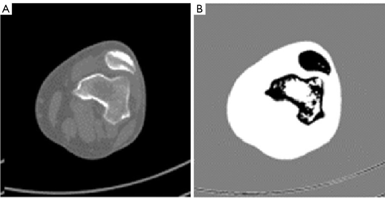
Here, represents the feature vector of the voxel, and represents the centroid of the cluster. The convergence criterion for this recalculation was defined as a change in centroid positions less than 0.001. The final membership degrees (Figure 5) were then used to assign voxels to the most suitable cluster.
Figure 5.
Image processing using FCM. (A) Original DICOM image. (B) Membership degree values produced by FCM, highlighting distinct regions of interest. FCM, fuzzy C-means; DICOM, Digital Imaging and Communications in Medicine.
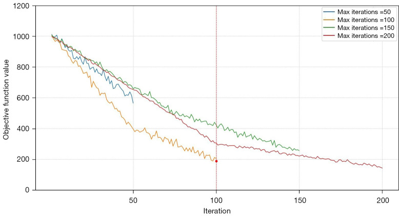
The FCM algorithm uses a set of input parameters, including the number of clusters, fuzziness parameter, and termination criterion, to iteratively assign each voxel to a specific cluster subject to its membership degree. For our study, the algorithm was configured with three clusters and a fuzziness parameter (m) of 2. These parameters were selected to achieve a balance between segmentation accuracy and computational efficiency. We evaluated the algorithm’s performance across various iteration limits: 50, 100, 150, and 200 iterations. Our analysis revealed that clustering results generally converged within 100 iterations for most datasets. Increasing the iteration limit beyond 100 did not substantially improve clustering performance, but did lead to increased computational time. Conversely, setting the iteration limit below 100 sometimes led to premature convergence and suboptimal clustering. Hence, a maximum of 100 iterations was determined to be optimal, offering a practical balance between accuracy and computational cost. Additionally, a convergence criterion of 0.001 was used to ensure the algorithm’s convergence.
Further evaluation of stability and convergence involved plotting the objective function’s trajectory across varying iteration limits (Figure 6). This plot highlights that the algorithm typically stabilizes within 100 iterations, reinforcing the necessity of allowing the full iteration process to achieve consistent performance. Additionally, we visualized the clustering results using a 3D scatter plot for 100 iterations (Figure 7). This visualization illustrates the distribution of data points across clusters and the positions of the centroids, demonstrating the FCM algorithm’s proficiency in producing well-defined and accurate clusters. The following steps summarized the algorithm:
Figure 6.
Convergence of the FCM objective function for different iteration limits. FCM, fuzzy C-means.
Figure 7.
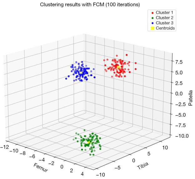
3D scatter plot illustrating clustering results obtained using FCM with 100 iterations. 3D, three-dimensional; FCM, fuzzy C-means.
Start by initializing the number of clusters (c) and the fuzziness parameter (m);
Randomly select (c) centroids (this involves choosing initial cluster centers randomly from the data points, which serves as the starting point for the clustering process);
Calculate the membership degrees of each voxel using the above equation;
Update the centroids of each cluster using the membership degrees;
Repeat steps 3–4 until convergence is achieved, i.e., until the algorithm has found stable centroids and membership degrees.
Once the FCM algorithm is applied, the region-based active contour approach will use the resulting membership degrees as an input to enhance the segmentation results and obtain a more accurate delineation of the knee bone boundaries.
Adaptive region-based ACM with customized energy function
To further enhance the knee bone boundary segmentation accuracy, we used an adaptive region-based ACM. By leveraging the specialized region descriptor provided by FCM, our model guides the contour’s movement to precisely identify the ROI. The integration of the adaptive region-based ACM with FCM clustering not only improves segmentation accuracy but also enhances computational efficiency. Our approach builds upon the methodology proposed by Chan-Vese (51) and is implemented through the following steps:
-
Define fitting energy function: the energy function quantifies the alignment between the evolving contour and the adjacent image intensities. The energy function is expressed as:
[7] Here, ϕ represents the level-set function, with µ, ν, and λ being weighting parameters that balance internal and external energy terms. A Gaussian kernel with a standard deviation σ is used to preserve image smoothness and gradient information. The parameter α controls the level of edge attraction.
-
Integrate the regularization term: the energy function is integrated with a regularization term to ensure precise and stable contour evolution. The variational level-set formulation is given by:
[8] where, κ is the curvature of the level-set function, and H is the Heaviside function.
- Formulate the evolving curve equation: the Euler-Lagrange equation is utilized for energy minimization, resulting in the evolving curve equation:
[9] Iteratively apply the gradient descent algorithm: the gradient descent algorithm is iteratively applied to optimize the energy function and obtain the optimal contour, ensuring efficient and accurate scientific image analysis.
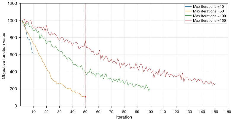
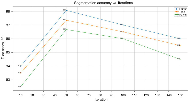
In our study, the parameters µ, ν, λ, α were set to 0.1, 0.9, 0.2, and 0.5, respectively, to balance internal and external energy terms. The regularization parameter δ was set to 1.0 to ensure stability and convergence of the contour evolution. A maximum of 50 iterations were allowed to optimize the energy function and obtain precise segmentation results. Figure 8 illustrates the convergence behavior of our algorithm across various iteration limits (10, 50, 100, and 150). The results demonstrate that 50 iterations yield the minimum objective function value, indicating optimal performance in terms of convergence efficiency and precision. Figure 9 presents the segmentation accuracy (Dice scores) for the femur, tibia, and patella across different iteration counts. The Dice scores notably increase from 10 to 50 iterations and then stabilize, suggesting that additional iterations beyond 50 do not significantly improve accuracy but may increase computational overhead. These results validate our parameter settings and iteration limits, highlighting their effectiveness in precise and efficient knee bone boundaries segmentation. Additionally, we tested various parameter values to assess the robustness of our method. We found that increasing µ and ν improved contour smoothness and stability, particularly in noisy regions, but sometimes led to a loss of fine details. While, higher λ and α alues enhanced the contour’s adherence to object boundaries, which was advantageous for images with clear edges but could cause instability in highly textured regions. The final segmentation results, as shown in Figure 10, demonstrate the model’s ability to achieve precise and accurate delineation of knee bone boundaries.
Figure 8.
Convergence of the region-based active contour model energy function over different iteration limits.
Figure 9.
Segmentation accuracy as measured by the Dice score for femur, tibia, and patella over different iteration counts.
Figure 10.
Segmentation results using an adaptive region-based active contour model. The femur, tibia, and patella are color-coded in red, blue, and green, respectively. The results are displayed across different views: (A) sagittal, (B) coronal, and (C) axial.
3D reconstruction of the knee bone
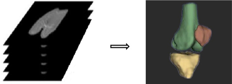
The knee joint segmentation results were utilized to generate a 3D volumetric rendering using the marching cubes algorithm (52). This process involved converting the contour data into a 3D matrix, creating a spatial model of the knee bone. Each voxel in this matrix represents a distinct element in the spatial domain. The iso-surface for each voxel was computed based on the threshold value or contour level, effectively delineating the boundary of the knee bone. The marching cubes algorithm efficiently generated the surface of the knee bone using triangular facets, enabling enhanced visualization of its spatial structure. Figure 11 presents the resulting 3D volumetric rendering, with the x- and y-axes correspond to the x- and y-pixels of the image, while the z-axis represents the pixel height of the knee bone.
Figure 11.
3D reconstruction of knee joint model. 3D, three-dimensional.
Results
Segmentation results
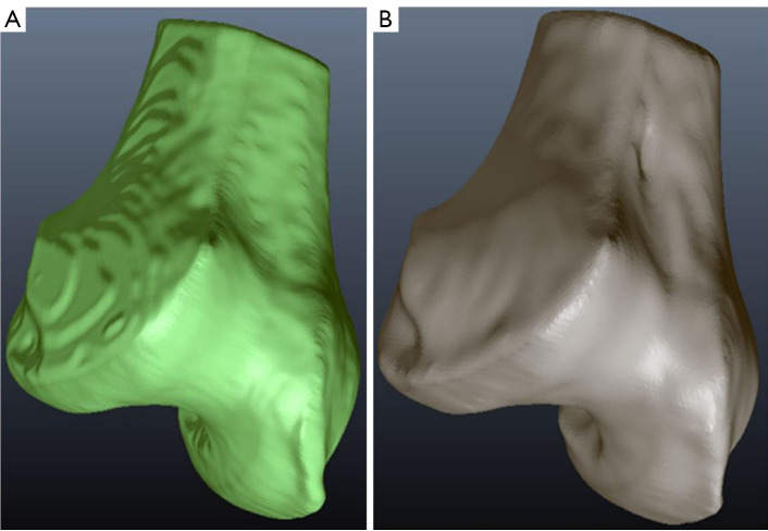
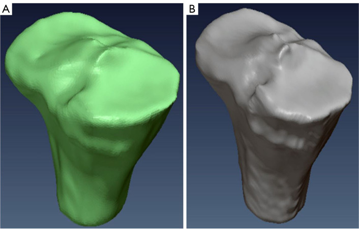
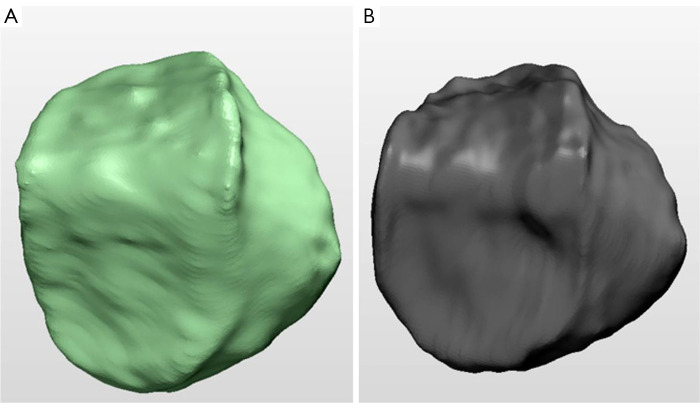
We evaluated the accuracy and reliability of our proposed method by comparing its segmentation results with those obtained from manual segmentation performed by two expert annotators using the 3D Slicer software. This comparison served as a reliable benchmark to assess the effectiveness and reliability of our approach, which can be seen in Figures 12-14.
Figure 12.
Comparative analysis of femur bone segmentation. (A) Automated segmentation using FCM and region-based ACM; (B) manual segmentation. FCM, fuzzy C-means; ACM, active contour model.
Figure 13.
Comparative analysis of tibia bone segmentation. (A) Automated segmentation using FCM and region-based ACM; (B) manual segmentation. FCM, fuzzy C-means; ACM, active contour model.
Figure 14.
Comparative analysis of tibia bone segmentation. (A) Automated segmentation using FCM and region-based ACM; (B) manual segmentation. FCM, fuzzy C-means; ACM, active contour model.
Morphological quantitative assessment
We performed a quantitative validation to evaluate the performance of our segmentation method. For this purpose, we randomly selected six CT image stacks, each representing a distinct knee joint. Manual segmentation of the bone regions was performed on each image, serving as the ground-truth reference for comparison. We utilized established metrics, including the DSC, sensitivity, and specificity, to assess the reliability of our segmented models (53). The choice of metrics was deliberate and directly aligned with the objectives of our study. The DSC quantifies the degree of overlap between the segmented knee bone region and the ground-truth reference, serving as a key measure of segmentation accuracy. Sensitivity, assesses the method’s ability to correctly identify knee bone regions, reducing the likelihood of missing true positive (TP) regions. Specificity, evaluates the method’s capacity to avoid false positives (FP), ensuring that non-knee bone regions are correctly identified. The mathematical formulations of these evaluation metrics are as follows:
| [10] |
| [11] |
| [12] |
In the above equations, TP denotes the accurately identified bone tissue region, false negative (FN) signifies the incorrectly identified non-bone tissue region, FP represents the erroneously identified bone tissue region and true negative (TN) corresponds to the correctly identified non-bone tissue region.
Table 1 provides the Dice statistics for the segmented knee bone across the selected dataset. The Dice scores ranged from 95.99% to 98.95%, demonstrating a high level of concordance and precision in segmenting the bone regions. These values, notably high within the field of medical imaging, affirm the effectiveness and reliability of our method. The high Dice scores for the femur and tibia are indicative of their relatively simpler geometry and larger size, which the algorithm can segment with greater consistency. However, the patella, due to its smaller and more complex structure, exhibited slightly lower Dice scores. This suggests that finer anatomical details present additional challenges, leading to minor deviations in segmentation performance.
Table 1. Dice score values for femur, tibia and patella.
| Dataset | Femur (%) | Tibia (%) | Patella (%) |
|---|---|---|---|
| 1 | 98.61 | 97.67 | 97.14 |
| 2 | 98.31 | 97.14 | 96.67 |
| 3 | 97.56 | 96.84 | 96.41 |
| 4 | 98.95 | 98.10 | 96.92 |
| 5 | 97.33 | 96.75 | 95.99 |
| 6 | 97.48 | 97.60 | 96.89 |
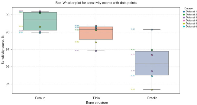
Table 2 provides the sensitivity scores for the segmented knee bone regions. These scores illustrate the method’s effectiveness in identifying TP regions within the dataset. Sensitivity scores for the femur ranged from 97.96% to 99.21%, demonstrating high accuracy in identifying femur regions. This high sensitivity is attributed to the distinct shape and clear boundary contrast of the femur in CT images. The tibia achieved sensitivity scores between 96.92% and 98.36%, reflecting reliable detection, with slight variation due to its elongated structure. Sensitivity scores for the patella ranged from 94.68% to 98.15%, indicating successful identification despite challenges such as partial volume effects and its articulating position with the femur. Figure 15 illustrates the distribution and variability of sensitivity scores across different bone regions using box-whisker plots.
Table 2. Sensitivity score values for femur, tibia and patella.
| Dataset | Femur (%) | Tibia (%) | Patella (%) |
|---|---|---|---|
| 1 | 99.16 | 98.23 | 98.15 |
| 2 | 99.10 | 98.11 | 96.97 |
| 3 | 98.04 | 96.92 | 95.74 |
| 4 | 99.21 | 98.36 | 96.67 |
| 5 | 98.31 | 97.41 | 94.68 |
| 6 | 97.96 | 98.33 | 95.45 |
Figure 15.
Box-whisker plot illustrating sensitivity scores for segmented knee bone regions. The plot visualizes the distribution of sensitivity scores for femur, tibia, and patella.
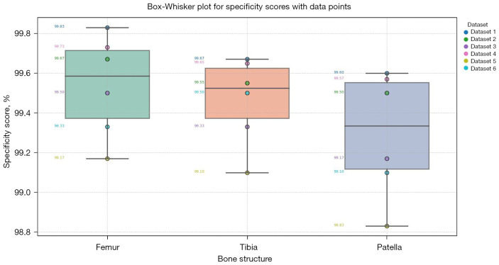
Table 3 provides the specificity scores for the segmented knee bone regions. Our method achieved average specificity scores of 99.67%, 99.50%, and 99.33% for the femur, tibia, and patella, respectively. These high specificity scores reflect the method’s effectiveness in accurately distinguishing non-bone tissue from the targeted regions. The specificity scores, consistently above 99%, reflect the algorithm’s robustness in avoiding FP and ensuring that non-bone structures are correctly identified and excluded from the segmented regions. The slightly lower specificity for the patella compared to the femur and tibia suggests that the patella’s complex interface with surrounding tissues can occasionally be misinterpreted, leading to a marginal increase in FP rates. However, these differences are minimal, underscoring the overall high performance and reliability of our segmentation method. Figure 16 presents box-whisker plots of the specificity scores, confirming the method’s robust performance.
Table 3. Specificity score values for femur, tibia and patella.
| Dataset | Femur (%) | Tibia (%) | Patella (%) |
|---|---|---|---|
| 1 | 99.83 | 99.67 | 99.60 |
| 2 | 99.67 | 99.55 | 99.50 |
| 3 | 99.50 | 99.33 | 99.17 |
| 4 | 99.73 | 99.65 | 99.57 |
| 5 | 99.17 | 99.10 | 98.83 |
| 6 | 99.33 | 99.50 | 99.10 |
Figure 16.
Box-whisker plots illustrating the specificity scores for segmented knee bone regions. The plot visualizes the distribution of specificity scores for femur, tibia, and patella.
Overall, our method’s performance, as reflected in the Dice coefficients, sensitivity, and specificity scores, demonstrates its robustness and precision in knee bone segmentation. The slight variations in performance across different bone structures are consistent with the inherent anatomical and imaging challenges. Our results highlight the effectiveness and clinical applicability of our method in providing accurate delineations of knee bone structures in CT imaging.
Geometrical accuracy assessment
Despite achieving an impressive Dice score of 98%, a more comprehensive evaluation of segmentation accuracy was imperative through geometric validation. To validate geometric precision of our segmentation approach, we implemented the Iterative Closest Point (ICP) algorithm (54) to register and align the segmented bone surfaces with a reference model. The geometric accuracy was quantitatively evaluated using the root mean square distance (RSD), as defined in Eq. [13] (55).
| [13] |
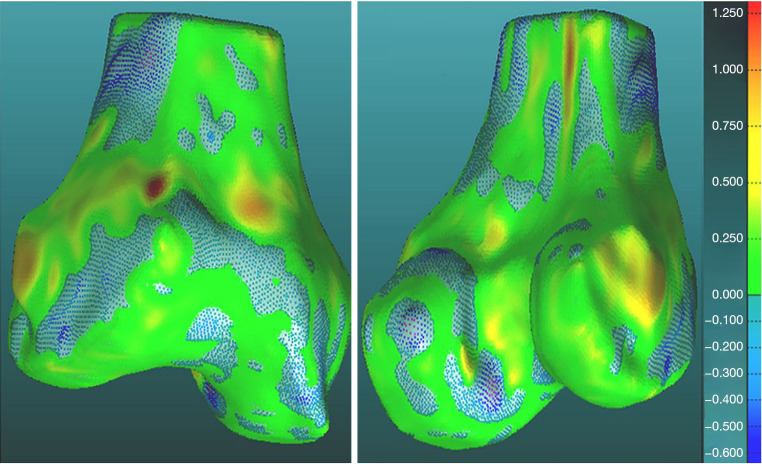
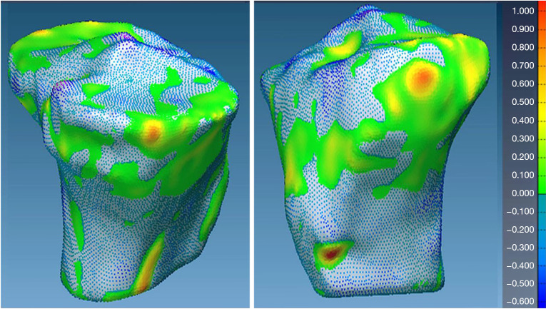
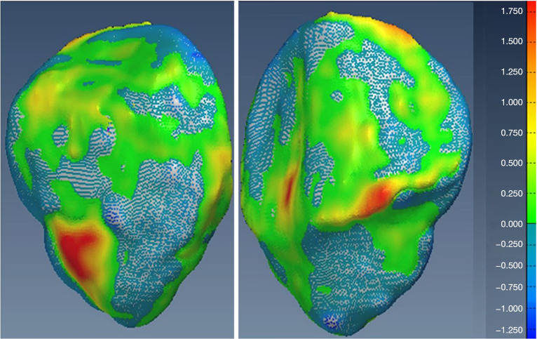
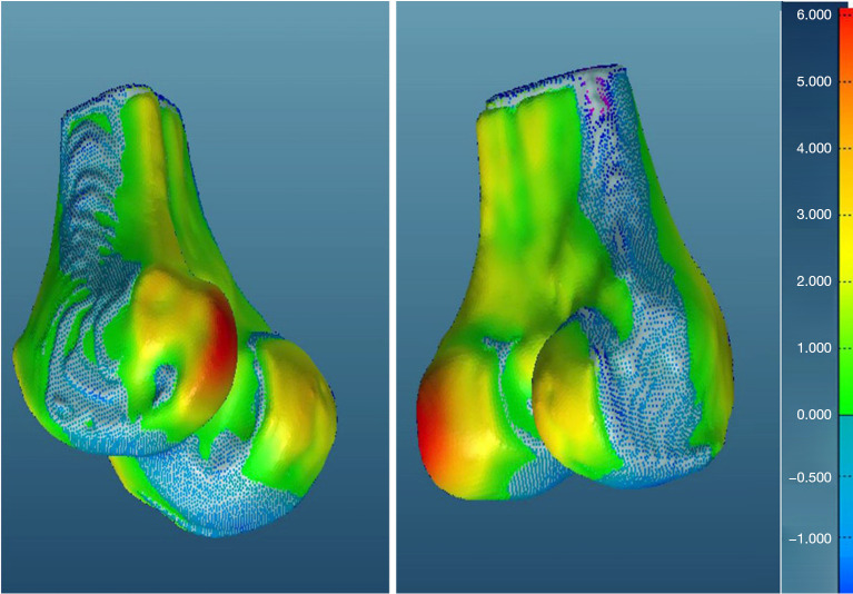
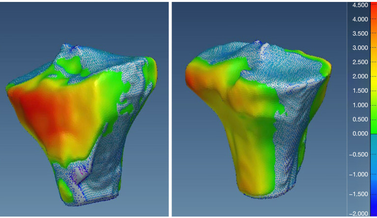
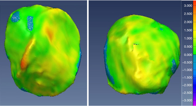
The comparison involved evaluating segmented models against manually segmented ground-truth models. Differences in mesh geometry between the two models were visualized using a color-coded scale, which highlighted variations in shape and structure. Geometric validation was performed on all six randomly selected datasets. The RSD values were computed for the femur, tibia, and patella across all datasets. Table 4 summarizes the RSD values for each bone model.
Table 4. Geometrical accuracy (RSD) values for femur, tibia and patella.
| Dataset | Femur RSD (mm) | Tibia RSD (mm) | Patella RSD (mm) |
|---|---|---|---|
| 1 | 0.51 | 0.49 | 0.59 |
| 2 | 0.49 | 0.53 | 0.61 |
| 3 | 0.52 | 0.48 | 0.58 |
| 4 | 0.50 | 0.50 | 0.60 |
| 5 | 0.48 | 0.52 | 0.62 |
| 6 | 0.53 | 0.47 | 0.57 |
RSD, root mean square distance; mm, millimeters.
The RSD values indicate the geometric differences for the femur, tibia, and patella models across the datasets. The average RSD values were 0.5±0.0183 mm for the femur, 0.5±0.0213 mm for the tibia, and, 0.6±0.0163 mm for the patella. These results demonstrate the high geometric accuracy of our method, with minimal deviations from the manually segmented ground-truth models. The spatial resolution of the CT images was 0.5 mm per pixel, which is sufficiently fine to capture detailed anatomical features. The observed RSD values are close to the pixel size, confirming that the segmentation accuracy aligns closely with the inherent resolution of the imaging data.
Additionally, visual inspection of the segmented models (Figures 17-22) further validated our method. The color-coded error maps did not reveal significant over- or underestimation in any specific regions, demonstrating consistent performance across the entire bone structures.
Figure 17.
Geometric validation of femur bone 3D mesh using color-coded map for Case 1. 3D, three-dimensional.
Figure 18.
Geometric validation of tibia bone 3D mesh using color coded map for Case 1. 3D, three-dimensional.
Figure 19.
Geometric validation of patella bone 3D mesh using color coded map for Case 1. 3D, three-dimensional.
Figure 20.
Geometric validation of femur bone 3D mesh using color coded map for Case 2. 3D, three-dimensional.
Figure 21.
Geometric validation of tibia bone 3D mesh using color coded map for Case 2. 3D, three-dimensional.
Figure 22.
Geometric validation of patella bone 3D mesh using color coded map for Case 2. 3D, three-dimensional.
Computational time efficiency
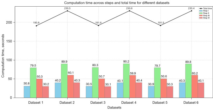
Computational efficiency is crucial for the practical implementation of medical image analysis algorithms. To evaluate the performance of our knee bone segmentation method, we conducted a detailed evaluation on a dedicated system equipped with an Intel® Core (TM) i5-1115G4 CPU, 16GB of RAM, and a 64-bit Windows 10 environment. We measured the execution time for each step of our algorithm to determine its overall computational efficiency. In Step 1, we applied preprocessing techniques, including Canny edge detection and Gaussian filtering, to enhance the image quality and prepare it for segmentation. Step 2 involved using FCM to classify pixels and separate knee bone structures from surrounding tissues. In Step 3, a region-based ACM was employed to refine the initial segmentation obtained from Step 2, ensuring accurate delineation of the knee bone structures. Finally, in Step 4, we used the marching cubes algorithm to reconstruct the segmented knee bone structure in three dimensions.
Considering the inherent complexity of knee bone segmentation and the variability in the number of slices per dataset (ranging from 100 to 300), the average total execution time per dataset ranged from approximately 190 to 230 seconds. Figure 23 illustrates the efficiency of our methodology, as it achieves accurate segmentation results within a reasonable timeframe, making it suitable for clinical settings.
Figure 23.
Execution time (seconds) for each step of our framework, highlighting the method’s computational efficiency across different image series.
Completeness & accuracy of segmentation
Completeness of the segmented knee bone region
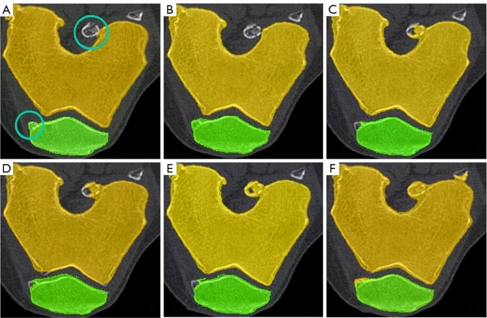
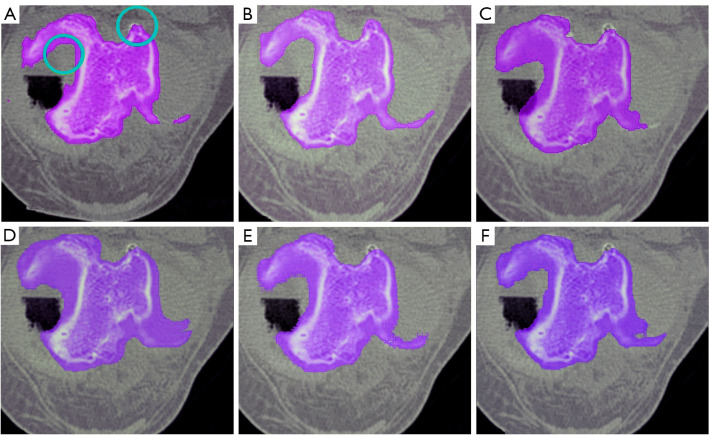
A critical concern in knee bone segmentation is the ability to accurately encompass the entire knee bone region. Our methodology addresses this concern comprehensively through an iterative process. Initially, the FCM clustering algorithm segments the image into clusters based on voxel intensity similarities. This step helps in distinguishing the knee bone components (femur, tibia, and patella) from other tissues. Subsequently, the adaptive region-based ACM refines these initial clusters by incorporating spatial continuity and boundary regularization. By iteratively updating membership degrees and centroids based on voxel similarities, our algorithm adeptly identifies and assigns voxels to their corresponding clusters. This process ensures that even in the presence of missing regions, the algorithm can adaptively adjust to capture the entire knee bone region accurately. The completeness of segmentation is visually confirmed in Figures 24,25, where our method is compared against other state-of-the-art segmentation techniques. Our method demonstrates superior performance in maintaining completeness of the knee bone region.
Figure 24.
Comparison of segmentation results for femur and patella bones in CT images with missing regions. (A) Manually segmented, (B) proposed method, (C) CPSM, (D) atlas-based, (E) ASM, and (F) deformable model. CT, computed tomography; CPSM, coupled prior shape model; ASM, active shape model.
Figure 25.
Comparison of segmentation results for tibial bone in CT images with missing regions. (A) Manually segmented, (B) proposed method, (C) CPSM, (D) atlas-based, (E) ASM, and (F) deformable model. CT, computed tomography; CPSM, coupled prior shape model; ASM, active shape model.
Accuracy of the segmentation boundaries
Another key aspect is the fidelity of the segmented boundaries in aligning with the true anatomical contours of the knee bone. We scrutinized the potential for deviations or inconsistencies in the segmentation results. Our methodology excels in achieving highly accurate segmentation boundaries that closely adhere to the true anatomical contours of the knee bone. The FCM algorithm performs precise clustering by analyzing voxel similarities in a multidimensional feature space, effectively distinguishing the knee bone components from surrounding tissues.
Furthermore, the region-based ACM iteratively optimizes the active contour to align closely with the true anatomical boundaries. This is achieved by minimizing an energy function that balances internal forces (smoothness of the contour) and external forces (image gradient and intensity information). The regularization term ensures that the contour evolves smoothly while accurately adhering to the bone boundaries. Minor deviations or inconsistencies, which may arise due to inherent variations in the image data or limitations in the segmentation process, have minimal impact on the overall accuracy and reliability of the segmentation results. This boundary accuracy is illustrated in Figures 24,25, where the segmented contours closely match the manual annotations by expert annotators.
Comparison with other state-of-the-art methods
To validate the accuracy of our bone region segmentation method, we conducted a benchmarking process against established image segmentation techniques using the Dice score metric for quantitative assessment. This comparison involved adapting MRI-based segmentation techniques for CT data, requiring specific preprocessing steps such as intensity normalization, noise reduction through filtering, and adjustments to algorithm parameters tailored to CT imaging characteristics. These steps were crucial to optimize our method’s performance given the higher contrast and noise levels typically encountered in CT compared to MRI.
For instance, methods by Shan et al. (56) and Fripp et al. (57) incorporated prior data and pre-defined models, which may not generalize well to the varied intensity profiles and artifacts present in CT images. This limitation can lead to under-segmentation or over-segmentation, especially in regions with ambiguous boundaries or overlapping tissue structures. Our approach operates independently of prior data, offering flexibility and broader applicability in diverse clinical settings. Additionally, Zhou et al. (58) focused exclusively on single MRI sequences, which are computationally intensive and less adaptable to the high-resolution and varied intensity characteristics of CT datasets. The computational complexity and specificity to MRI sequences limit their practical application to CT images, where our method demonstrates a significant advantage in both performance and computational efficiency. Pang et al. (59) reported average surface distances primarily for specific slice locations rather than comprehensive measurements across the entire bone surface, making it challenging to assess their method’s effectiveness on full volumes.
Table 5 provides a detailed comparison of our results with recent studies, demonstrating that our method consistently achieves high average Dice scores across the six randomly selected cases. However, direct comparisons are nuanced due to differences in methodologies, imaging modalities, and dataset characteristics. These results indicate that our method performs at a comparable or superior level to the other methods, underscoring both the high anatomical fidelity and robustness of our segmentation approach.
Table 5. Comparison of mean Dice values among proposed method and other benchmark methods.
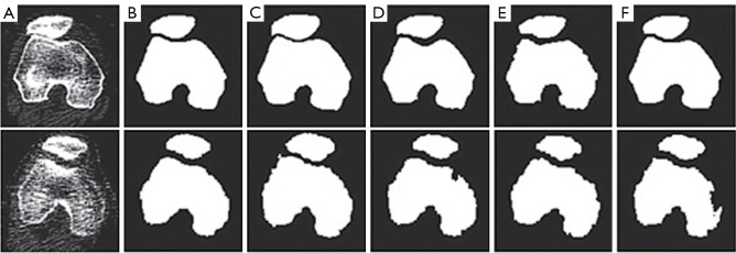
Figure 26 visually compares our method’s segmentation outcomes with those of various approaches. Our method consistently exhibits sharper and more precise delineation of bone regions, showcasing robustness in handling challenges like soft tissue variations, intensity irregularities, and noise inherent in CT images. This improvement is attributed to advanced clustering algorithms and contour refinement techniques that effectively preserve bone boundaries and minimize segmentation errors.
Figure 26.
Comparison of segmentation results for two cases using the proposed method and other methods. (A) Manually segmented, (B) proposed method, (C) CPSM, (D) atlas-based, (E) ASM, and (F) deformable model. CT, computed tomography; CPSM, coupled prior shape model; ASM, active shape model.
Discussion
In this study, we presented a semi-automatic method for segmenting multiple knee bones from CT images. Our approach combines various image preprocessing techniques, including canny edge detection and gaussian filtering, with advanced algorithms such as FCM, region-based ACM, and marching cubes for 3D reconstruction (60).
The methodology begins with the application of Canny edge detection and Gaussian filtering to enhance image quality by emphasizing significant edge features. The FCM algorithm is then used to classify pixels into distinct tissue classes, considering the uncertainty associated with tissue intensity variations and overlapping regions. This classification provided an initial segmentation, which was then refined using a region-based ACM. The ACM iteratively adjusted the contours by minimizing an energy function that integrated both image-based and geometric priors, ensuring precise delineation of the knee bone boundaries. Finally, the marching cubes algorithm was employed to reconstruct the 3D model of the segmented bone regions, enabling enhanced visualization and providing critical support for accurate diagnosis and treatment planning (61).
The quantitative evaluation of our method, using well-established benchmark metrics, including the Dice, sensitivity, and specificity, demonstrated its exceptional performance. The obtained high Dice scores for the femur (98.95%), tibia (98.10%), and patella (97.14%) underscore the remarkable overlap between the segmented regions and the corresponding ground truth manual segmentations. These results strongly affirm the reliability and accuracy of our methodology (62).
Further validation was conducted through geometrical validation, focusing on the alignment and geometric similarity of the segmented bone surfaces. Utilizing the ICP algorithm, we registered the segmented surfaces and computed the RSD to quantify geometric differences. The low RSD values for the tibia and femur (0.5±0.14 mm) and patella (0.6±0.13 mm) highlight the method’s ability to accurately capture the intricate geometries of knee bone structures with high consistency (63).
Conclusions
In conclusion, our study presents an advanced integration of the FCM algorithm with an adaptive region-based ACM for the segmentation of knee joints from CT images. This approach has demonstrated exceptional accuracy and efficiency, making it a valuable tool for precise orthopedic surgery planning. The results provide distinct and non-overlapping segmentation of knee bones, highlighting its clinical relevance and applicability. However, several challenges and limitations must be considered. A key limitation is the dependency on image preprocessing techniques, which, although essential for enhancing image quality, may inadvertently introduce noise or artifacts that could compromise segmentation accuracy. Furthermore, the current study does not fully explore the method’s performance in pathological cases, where abnormal bone structures might present significant challenges. While this study has focused on knee bone segmentation, future research could explore the segmentation and geometrical modeling of other anatomical structures within the knee joint, such as ligaments and cartilage. Moreover, to establish the clinical utility of our segmentation framework, rigorous clinical trials involving orthopedic surgeons and radiologists are essential. These trials would evaluate the method’s integration into routine clinical practice and its impact on improving surgical outcomes. By addressing these limitations, we aim to enhance the robustness and clinical applicability of our segmentation method.
Supplementary
The article’s supplementary files as
Acknowledgments
The authors express their gratitude to all the staff at the Second Affiliated Hospital of Dalian Medical University for their support during this research.
Funding: None.
Ethical Statement: The authors are accountable for all aspects of the work in ensuring that questions related to the accuracy or integrity of any part of the work are appropriately investigated and resolved. The study was conducted in accordance with the Declaration of Helsinki (as revised in 2013) and informed consent was obtained from all volunteers who participated in the study. Ethical approval for this study was waived by the ethics committee of Second Affiliated Hospital of Dalian Medical University.
Footnotes
Conflicts of Interest: All authors have completed the ICMJE uniform disclosure form (available at https://qims.amegroups.com/article/view/10.21037/qims-24-821/coif). The authors have no conflicts of interest to declare.
References
- 1.Kishore VV, Dosapati UB, Deekshith E, Boyapati K, Pranay S, Kalpana V. CAD Tool for Prediction of Knee Osteoarthritis (KOA). 2024 10th International Conference on Communication and Signal Processing (ICCSP), Melmaruvathur, India, 2024:18-23. [Google Scholar]
- 2.Starmans MP, van der Voort SR, Tovar JMC, Veenland JF, Klein S, Niessen WJ. Radiomics: data mining using quantitative medical image features. Handbook of medical image computing and computer assisted intervention. Academic Press, 2020:429-56. [Google Scholar]
- 3.Chen H, Sprengers AMJ, Kang Y, Verdonschot N. Automated segmentation of trabecular and cortical bone from proton density weighted MRI of the knee. Med Biol Eng Comput 2019;57:1015-27. 10.1007/s11517-018-1936-7 [DOI] [PMC free article] [PubMed] [Google Scholar]
- 4.Walker PS. The Artificial Knee: An Ongoing Evolution. Springer, 2020. [Google Scholar]
- 5.Poliakov A, Pakhaliuk V, Popov VL. Current trends in improving of artificial joints design and technologies for their arthroplasty. Front Mech Eng 2020;6:4. [Google Scholar]
- 6.Coaccioli S, Sarzi-Puttini P, Zis P, Rinonapoli G, Varrassi G. Osteoarthritis: New Insight on Its Pathophysiology. J Clin Med 2022;11:6013. 10.3390/jcm11206013 [DOI] [PMC free article] [PubMed] [Google Scholar]
- 7.Kim CW, Lee CR, Seo YC, Seo SS. Total knee arthroplasty. A Strategic Approach to Knee Arthritis Treatment: From Non-Pharmacologic Management to Surgery 2021:273-364.
- 8.Mijiritsky E, Ben Zaken H, Shacham M, Cinar IC, Tore C, Nagy K, Ganz SD. Variety of Surgical Guides and Protocols for Bone Reduction Prior to Implant Placement: A Narrative Review. Int J Environ Res Public Health 2021;18:2341. 10.3390/ijerph18052341 [DOI] [PMC free article] [PubMed] [Google Scholar]
- 9.Sood C. Patient-specific Instrumentation in Total Knee Arthroplasty. In: Sharma M. editors. Knee Arthroplasty. Springer, Singapore, 2022:459-75. [Google Scholar]
- 10.Suneja A, Deshpande SV, Pisulkar G, Taywade S, Awasthi AA, Salwan A, Goel S. Navigating the Divide: A Comprehensive Review of the Mechanical and Anatomical Axis Approaches in Total Knee Replacement. Cureus 2024;16:e57938. 10.7759/cureus.57938 [DOI] [PMC free article] [PubMed] [Google Scholar]
- 11.Hohlmann B, Broessner P, Phlippen L, Rohde T, Radermacher K. Knee Bone Models From Ultrasound. IEEE Trans Ultrason Ferroelectr Freq Control 2023;70:1054-63. 10.1109/TUFFC.2023.3286287 [DOI] [PubMed] [Google Scholar]
- 12.Feng B, Zhu W, Bian YY, Chang X, Cheng KY, Weng XS. China artificial joint annual data report. Chin Med J (Engl) 2020;134:752-3. 10.1097/CM9.0000000000001196 [DOI] [PMC free article] [PubMed] [Google Scholar]
- 13.Gao J, Xing D, Dong S, Lin J. The primary total knee arthroplasty: a global analysis. J Orthop Surg Res 2020;15:190. 10.1186/s13018-020-01707-5 [DOI] [PMC free article] [PubMed] [Google Scholar]
- 14.Peñate Medina T, Kolb JP, Hüttmann G, Huber R, Peñate Medina O, Ha L, Ulloa P, Larsen N, Ferrari A, Rafecas M, Ellrichmann M, Pravdivtseva MS, Anikeeva M, Humbert J, Both M, Hundt JE, Hövener JB. Imaging Inflammation - From Whole Body Imaging to Cellular Resolution. Front Immunol 2021;12:692222. 10.3389/fimmu.2021.692222 [DOI] [PMC free article] [PubMed] [Google Scholar]
- 15.Demehri S, Baffour FI, Klein JG, Ghotbi E, Ibad HA, Moradi K, Taguchi K, Fritz J, Carrino JA, Guermazi A, Fishman EK, Zbijewski WB, Musculoskeletal CT. Imaging: State-of-the-Art Advancements and Future Directions. Radiology 2023;308:e230344. 10.1148/radiol.230344 [DOI] [PMC free article] [PubMed] [Google Scholar]
- 16.Martel-Pelletier J, Paiement P, Pelletier JP. Magnetic resonance imaging assessments for knee segmentation and their use in combination with machine/deep learning as predictors of early osteoarthritis diagnosis and prognosis. Ther Adv Musculoskelet Dis 2023;15:1759720X231165560. [DOI] [PMC free article] [PubMed]
- 17.Yao Y, Zhong J, Zhang L, Khan S, Chen W. CartiMorph: A framework for automated knee articular cartilage morphometrics. Med Image Anal 2024;91:103035. 10.1016/j.media.2023.103035 [DOI] [PubMed] [Google Scholar]
- 18.Ambellan F, Tack A, Ehlke M, Zachow S. Automated segmentation of knee bone and cartilage combining statistical shape knowledge and convolutional neural networks: Data from the Osteoarthritis Initiative. Med Image Anal 2019;52:109-18. 10.1016/j.media.2018.11.009 [DOI] [PubMed] [Google Scholar]
- 19.Wu J, Mahfouz MR. Reconstruction of knee anatomy from single-plane fluoroscopic x-ray based on a nonlinear statistical shape model. J Med Imaging (Bellingham) 2021;8:016001. 10.1117/1.JMI.8.1.016001 [DOI] [PMC free article] [PubMed] [Google Scholar]
- 20.Charon N, Islam A, Zbijewski W. Landmark-free morphometric analysis of knee osteoarthritis using joint statistical models of bone shape and articular space variability. J Med Imaging (Bellingham) 2021;8:044001. 10.1117/1.JMI.8.4.044001 [DOI] [PMC free article] [PubMed] [Google Scholar]
- 21.Ahmed SM, Mstafa RJ. A Comprehensive Survey on Bone Segmentation Techniques in Knee Osteoarthritis Research: From Conventional Methods to Deep Learning. Diagnostics (Basel) 2022;12:611. 10.3390/diagnostics12030611 [DOI] [PMC free article] [PubMed] [Google Scholar]
- 22.Patekar R, Kumar PS, Gan H-S, Ramlee MH. Automated Knee Bone Segmentation and Visualisation Using Mask RCNN and Marching Cube: Data from The Osteoarthritis Initiative. ASM Sci J 2022;17:1-7. [Google Scholar]
- 23.Chadoulos C, Tsaopoulos D, Symeonidis A, Moustakidis S, Theocharis J. Dense Multi-Scale Graph Convolutional Network for Knee Joint Cartilage Segmentation. Bioengineering (Basel) 2024;11:278. 10.3390/bioengineering11030278 [DOI] [PMC free article] [PubMed] [Google Scholar]
- 24.Pattanaik P, Alsubaie N, Alqahtani MS, Soufiene BO. A Novel Detection of Tibiofemoral Joint Kinematical Space using Graph-based Model of 3D Point Cloud Sequences. 2023. doi: .
- 25.Liu X, Song L, Liu S, Zhang Y. A review of deep-learning-based medical image segmentation methods. Sustainability 2021;13:1224. [Google Scholar]
- 26.Wang R, Lei T, Cui R, Zhang B, Meng H, Nandi AK. Medical image segmentation using deep learning: A survey. IET Image Process 2022;16:1243-67. [Google Scholar]
- 27.Kora P, Ooi CP, Faust O, Raghavendra U, Gudigar A, Chan WY, Meenakshi K, Swaraja K, Plawiak P, Acharya UR. Transfer learning techniques for medical image analysis: A review. Biocybern Biomed Eng 2022;42:79-107. [Google Scholar]
- 28.Dong D, Fu G, Li J, Pei Y, Chen Y. An unsupervised domain adaptation brain CT segmentation method across image modalities and diseases. Expert Syst Appl 2022;207:118016. [Google Scholar]
- 29.Xie W, Willems N, Patil S, Li Y, Kumar M, editors. SAM Fewshot Finetuning for Anatomical Segmentation in Medical Images. Proceedings of the IEEE/CVF Winter Conference on Applications of Computer Vision (WACV), 2024:3253-61. [Google Scholar]
- 30.Almajalid R, Zhang M, Shan J. Fully Automatic Knee Bone Detection and Segmentation on Three-Dimensional MRI. Diagnostics (Basel) 2022;12:123. 10.3390/diagnostics12010123 [DOI] [PMC free article] [PubMed] [Google Scholar]
- 31.Hohlmann B, Radermacher K. Augmented active shape model search—Towards 3D ultrasound-based bone surface reconstruction. Proc EPiC Ser Health Sci 2020;4:117-21. [Google Scholar]
- 32.Liu F. SUSAN: segment unannotated image structure using adversarial network. Magn Reson Med 2019;81:3330-45. 10.1002/mrm.27627 [DOI] [PMC free article] [PubMed] [Google Scholar]
- 33.du Toit C, Orlando N, Papernick S, Dima R, Gyacskov I, Fenster A. Automatic femoral articular cartilage segmentation using deep learning in three-dimensional ultrasound images of the knee. Osteoarthr Cartil Open 2022;4:100290. 10.1016/j.ocarto.2022.100290 [DOI] [PMC free article] [PubMed] [Google Scholar]
- 34.Hall ME, Black MS, Gold GE, Levenston ME. Validation of watershed-based segmentation of the cartilage surface from sequential CT arthrography scans. Quant Imaging Med Surg 2022;12:1-14. 10.21037/qims-20-1062 [DOI] [PMC free article] [PubMed] [Google Scholar]
- 35.Liu F, Zhou Z, Jang H, Samsonov A, Zhao G, Kijowski R. Deep convolutional neural network and 3D deformable approach for tissue segmentation in musculoskeletal magnetic resonance imaging. Magn Reson Med 2018;79:2379-91. 10.1002/mrm.26841 [DOI] [PMC free article] [PubMed] [Google Scholar]
- 36.Liu H, Sun Y, Cheng X, Jiang D. Prior-Based 3D U-Net: A model for knee-cartilage segmentation in MRI images. Comput Graph 2023;115:167-80. [Google Scholar]
- 37.Li W, Xiao Z, Liu J, Feng J, Zhu D, Liao J, Yu W, Qian B, Chen X, Fang Y, Li S. Deep learning-assisted knee osteoarthritis automatic grading on plain radiographs: the value of multiview X-ray images and prior knowledge. Quant Imaging Med Surg 2023;13:3587-601. 10.21037/qims-22-1250 [DOI] [PMC free article] [PubMed] [Google Scholar]
- 38.Mahum R, Rehman SU, Meraj T, Rauf HT, Irtaza A, El-Sherbeeny AM, El-Meligy MA. A Novel Hybrid Approach Based on Deep CNN Features to Detect Knee Osteoarthritis. Sensors (Basel) 2021;21:6189. 10.3390/s21186189 [DOI] [PMC free article] [PubMed] [Google Scholar]
- 39.Norman B, Pedoia V, Majumdar S. Use of 2D U-Net Convolutional Neural Networks for Automated Cartilage and Meniscus Segmentation of Knee MR Imaging Data to Determine Relaxometry and Morphometry. Radiology 2018;288:177-85. 10.1148/radiol.2018172322 [DOI] [PMC free article] [PubMed] [Google Scholar]
- 40.Chadoulos CG, Tsaopoulos DE, Moustakidis S, Tsakiridis NL, Theocharis JB. A novel multi-atlas segmentation approach under the semi-supervised learning framework: Application to knee cartilage segmentation. Comput Methods Programs Biomed 2022;227:107208. 10.1016/j.cmpb.2022.107208 [DOI] [PubMed] [Google Scholar]
- 41.Gandhamal A, Talbar S, Gajre S, Razak R, Hani AFM, Kumar D. Fully automated subchondral bone segmentation from knee MR images: Data from the Osteoarthritis Initiative. Comput Biol Med 2017;88:110-25. 10.1016/j.compbiomed.2017.07.008 [DOI] [PubMed] [Google Scholar]
- 42.Cheng R, Alexandridi NA, Smith RM, Shen A, Gandler W, McCreedy E, McAuliffe MJ, Sheehan FT. Fully automated patellofemoral MRI segmentation using holistically nested networks: Implications for evaluating patellofemoral osteoarthritis, pain, injury, pathology, and adolescent development. Magn Reson Med 2020;83:139-53. 10.1002/mrm.27920 [DOI] [PMC free article] [PubMed] [Google Scholar]
- 43.Chen P, Gao L, Shi X, Allen K, Yang L. Fully automatic knee osteoarthritis severity grading using deep neural networks with a novel ordinal loss. Comput Med Imaging Graph 2019;75:84-92. 10.1016/j.compmedimag.2019.06.002 [DOI] [PMC free article] [PubMed] [Google Scholar]
- 44.Peng Y, Zheng H, Liang P, Zhang L, Zaman F, Wu X, Sonka M, Chen DZ. KCB-Net: A 3D knee cartilage and bone segmentation network via sparse annotation. Med Image Anal 2022;82:102574. 10.1016/j.media.2022.102574 [DOI] [PMC free article] [PubMed] [Google Scholar]
- 45.Chadoulos CG, Tsaopoulos DE, Moustakidis SP, Theocharis JB. A Multi-View Semi-supervised learning method for knee joint cartilage segmentation combining multiple feature descriptors and image modalities. Comput Methods Biomech Biomed Eng Imaging Vis 2024;12:2332398. [Google Scholar]
- 46.Deschamps K, Eerdekens M, Geentjens J, Santermans L, Steurs L, Dingenen B, Thysen M, Staes F. A novel approach for the detection and exploration of joint coupling patterns in the lower limb kinetic chain. Gait Posture 2018;62:372-7. 10.1016/j.gaitpost.2018.03.051 [DOI] [PubMed] [Google Scholar]
- 47.Rahman A, Bandara WGC, Valanarasu JMJ, Hacihaliloglu I, Patel VM. Orientation-Guided Graph Convolutional Network for Bone Surface Segmentation. In: Wang L, Dou Q, Fletcher PT, Speidel S, Li S. editors. Medical Image Computing and Computer Assisted Intervention – MICCAI 2022. Lecture Notes in Computer Science, Springer, 2022;13435:412-21. [Google Scholar]
- 48.Kanthavel R, Dhaya R, Venusamy K. Detection of Osteoarthritis Based on EHO Thresholding. Comput Mater Contin 2022;71:5783-98. [Google Scholar]
- 49.Hashemi SE, Gholian-Jouybari F, Hajiaghaei-Keshteli M. A fuzzy C-means algorithm for optimizing data clustering. Expert Syst Appl 2023;227:120377. [Google Scholar]
- 50.Latif G, Alghazo J, Sibai FN, Iskandar DNFA, Khan AH. Recent Advancements in Fuzzy C-means Based Techniques for Brain MRI Segmentation. Curr Med Imaging 2021;17:917-30. 10.2174/1573405616666210104111218 [DOI] [PubMed] [Google Scholar]
- 51.Ruiying H. An Improved Chan-Vese Model. 2021 IEEE Asia-Pacific Conference on Image Processing, Electronics and Computers (IPEC), Dalian, China, 2021:765-8. [Google Scholar]
- 52.Wang X, Gao S, Wang M, Duan Z. A marching cube algorithm based on edge growth. Virtual Reality & Intelligent Hardware 2021;3:336-49. [Google Scholar]
- 53.Müller D, Soto-Rey I, Kramer F. Towards a guideline for evaluation metrics in medical image segmentation. BMC Res Notes 2022;15:210. 10.1186/s13104-022-06096-y [DOI] [PMC free article] [PubMed] [Google Scholar]
- 54.Zhang J, Yao Y, Deng B. Fast and Robust Iterative Closest Point. IEEE Trans Pattern Anal Mach Intell 2022;44:3450-66. 10.1109/TPAMI.2021.3054619 [DOI] [PubMed] [Google Scholar]
- 55.Hodson To. Root mean square error (RMSE) or mean absolute error (MAE): When to use them or not. Geosci Model Dev 2022;2022:1-10. [Google Scholar]
- 56.Shan L, Zach C, Charles C, Niethammer M. Automatic atlas-based three-label cartilage segmentation from MR knee images. Med Image Anal 2014;18:1233-46. 10.1016/j.media.2014.05.008 [DOI] [PMC free article] [PubMed] [Google Scholar]
- 57.Fripp J, Crozier S, Warfield SK, Ourselin S. Automatic segmentation of the bone and extraction of the bone-cartilage interface from magnetic resonance images of the knee. Phys Med Biol 2007;52:1617-31. 10.1088/0031-9155/52/6/005 [DOI] [PubMed] [Google Scholar]
- 58.Zhou Z, Zhao G, Kijowski R, Liu F. Deep convolutional neural network for segmentation of knee joint anatomy. Magn Reson Med 2018;80:2759-70. 10.1002/mrm.27229 [DOI] [PMC free article] [PubMed] [Google Scholar]
- 59.Pang J, Driban JB, McAlindon TE, Tamez-Peña JG, Fripp J, Miller EL. On the use of coupled shape priors for segmentation of magnetic resonance images of the knee. IEEE J Biomed Health Inform 2015;19:1153-67. 10.1109/JBHI.2014.2329493 [DOI] [PMC free article] [PubMed] [Google Scholar]
- 60.Ebrahimkhani S, Jaward MH, Cicuttini FM, Dharmaratne A, Wang Y, de Herrera AGS. A review on segmentation of knee articular cartilage: from conventional methods towards deep learning. Artif Intell Med 2020;106:101851. 10.1016/j.artmed.2020.101851 [DOI] [PubMed] [Google Scholar]
- 61.Fan X, Zhu Q, Tu P, Joskowicz L, Chen X. A review of advances in image-guided orthopedic surgery. Phys Med Biol 2023. doi: . 10.1088/1361-6560/acaae9 [DOI] [PubMed] [Google Scholar]
- 62.Wang Z, Wang E, Zhu Y. Image segmentation evaluation: a survey of methods. Artif Intell Rev 2020;53:5637-74. [Google Scholar]
- 63.Fischer MCM, Grothues SAGA, Habor J, de la Fuente M, Radermacher K. A robust method for automatic identification of femoral landmarks, axes, planes and bone coordinate systems using surface models. Sci Rep 2020;10:20859. 10.1038/s41598-020-77479-z [DOI] [PMC free article] [PubMed] [Google Scholar]
Associated Data
This section collects any data citations, data availability statements, or supplementary materials included in this article.
Supplementary Materials
The article’s supplementary files as


