Empirical characterization of the expression ratio noise structure in high-density oligonucleotide arrays

Abstract

Background

High-density oligonucleotide arrays (HDONAs) are a powerful tool for assessing differential mRNA expression levels. To establish the statistical significance of an observed change in expression, one must take into account the noise introduced by the enzymatic and hybridization steps, called type I noise. We undertake an empirical characterization of the experimental repeatability of results by carrying out statistical analysis of a large number of duplicate HDONA experiments.

Results

We assign scoring functions for expression ratios and associated quality measures. Both the perfect-match (PM) probes and the differentials between PM and single-mismatch (MM) probes are considered as raw intensities. We then calculate the log-ratio of the noise structure using robust estimates of their intensity-dependent variance. The noise structure in the log-ratios follows a local log-normal distribution in both the PM and PM-MM cases. Significance relative to the type I noise can therefore be quantified reliably using the local standard deviation (SD). We discuss the intensity dependence of the SD and show that ratio scores greater than 1.25 are significant in the mid- to high-intensity range.

Conclusions

The noise inherent in HDONAs is characteristically dependent on intensity and can be well described in terms of local normalization of log-ratio distributions. Therefore, robust estimates of the local SD of these distributions provide a simple and powerful way to assess significance (relative to type I noise) in differential gene expression, and will be helpful in practice for improving the reliability of predictions from hybridization experiments.

Background

DNA microarray experiments have huge potential for screening for gene expression of relevance in particular contexts. However, the output of such an experiment is often just a list of 'fold-changes' in gene-expression levels and so researchers face the question of whether their 'hits' can be trusted or not. In the absence of any knowledge of what to expect, most researchers simply draw a line at a given fold-change and examine whatever is above it. The largest fold-changes in highly expressed genes can usually be trusted. However, because the 'correct' fold-change limit typically shifts with decreasing intensity of expression, a fixed fold-change line is inadequate in the range of expression levels where most genes actually lie. Most papers reporting microarray experiments cut off their candidate lists in essentially arbitrary ways, at the level that the researchers feel comfortable with, rather than on the basis of statistics. Here we present an easy but sound recipe for quantifying statistical significance, based on careful statistical characterization of a large dataset of GeneChip^® experiments.

A particular feature of GeneChip arrays is that each transcript is probed by many short snippets of sequence, instead of a single longer probe as in cDNA arrays [1,2,3]. Therefore, translating the measured probe intensities into a global gene-intensity or ratio score requires a composite scoring function. In principle, the redundancy in the probes offers a way to reduce the noise level for each gene; on the other hand, finding the best estimator is difficult and it is likely that the variability in probe behavior will prevent a single estimator from being optimal in all cases. Studying the raw data reveals its great complexity, and the hybridization processes underlying the measured perfect-match (PM) versus single-mismatch (MM) intensities prove hard to interpret physically. The principal difficulties stem first from the large number of probes with MM intensities higher than the corresponding PM, and therefore not conforming to the usual hybridization picture; and second, from the very broad intensity distributions within each probe set.

The first task is therefore to design a method that can robustly handle such input data. Second, once reliable measures for differential expression from two experiments are obtained, one would like to measure their significance level. It is now widely accepted that such measures should be derived in an intensity-dependent fashion [4,5,6,7,8]. There are at least two independent sources of variability to be considered: first, the intrinsic noise levels related to the technology (type I noise), which includes noise components introduced by the enzymatic step used in the cRNA preparation (see Materials and methods) and the fluorescence measurement (scan); and second, the variability encountered in biological replicates. Previous studies have addressed significance issues in both cDNA and GeneChip arrays: they have discussed significance according to intrinsic noise levels [4,5]; or focused on variability in replicates only [6,7]; or considered both simultaneously [8].

High-density oligonucleotide microarrays (HDONAs) are composed of 25-base oligonucleotide probes synthesized and attached to a glass matrix by photolithographic techniques. As such a short oligonucleotide sequence would not give sufficiently specific hybridization alone, GeneChip uses 14-20 different oligonucleotides to probe each transcript; and each comes in two versions - the PM probe and the MM probe. In the latter, the central base has been substituted by its complement and this probe is intended to control for nonspecificity. The pairs (PM, MM) are called probe pairs and the full set of probes for a given gene is called a probe set. The standard picture used to interpret the hybridization is based on the following model [2,9,10]:

PM = I_S + I_NS + B

MM = (1 - )I_S + 'I_NS + B

where PM (MM) is the observed brightness, I_S the contribution from specific complementary binding, I_NS the amount from nonspecific binding, and B a background of physical origin, that is, the photodetector dark current or light reflections from the scanning process. The proper technique for estimating the background and its fluctuations is discussed in [11]. Then, (thought to be positive) reflects the loss of binding due to a single substitution, and , ' are the susceptibilities for nonspecific binding. In the ideal case, which is usually assumed, = ' and therefore the subtraction PM - MM = (1 - )I_S is directly proportional to the desired signal. However, the susceptibility can be strongly varying within a given probe set.

We shall focus on the following two aspects of GeneChip data analysis: first, we describe a method to evaluate ratio scores and associated quality measures. In this step, we shall relax the assumption that = ' and consider either the PM probes only or the usual PM-MM subtraction. These cases were chosen to bracket the extremes of an ideally performing MM probe and a poor MM. Second, we use the assigned ratio scores and show how one can, with moderate effort, attribute a significance level to differentially expressed genes. Our approach is somewhat similar to that described in [8], in the sense that it relies on an empirical characterization of the noise envelope, and is more distantly related to that described in [5]. Both these approaches were developed and applied in the context of cDNA arrays (see Materials and methods for a discussion of the difference between our method and [8]).

Results

There are two types of approaches to composite scores: first, the 'direct' methods [2,11] aim at obtaining scores based on the distribution study of the probe intensities and can be applied to a single experiment (or pair in the case of ratio estimators); the second approach is model based [9,10] and attempts to fit the susceptibilities and from a collection of arrays. A major difference in the two methods is that the number of experiments needed can be just one (or two for ratios) in the first case, whereas a large number of arrays of similar quality (ideally as many as the number of probe pairs for the reduced model [9]) are required for the second. Model-based approaches seem to be well suited for absolute intensity measurements; on the other hand, direct methods are not expected to be very robust for absolute intensities, because of the broad intensity distributions within probe sets [11]. However, the situation is different when considering ratio scores, as the variability in the individual probe susceptibilities cancels out when considering the expression ratios at the probe level. Ratio scores should therefore be expected to be more robust; more precisely, when comparing two conditions, we consider each probe ratio to provide an independent measurement of the real expression ratio - independent in the sense that the 16 ratios provide independent samples from a distribution whose location we want to estimate. Our composite ratio estimation is based on a standard least trimmed square (LTS) estimator of the set of log-ratios for each probe set (see Materials and methods for details). We consider the cases for which the probe log-ratios (LR) are derived either from the usual PM-MM subtracted intensities, or from the PM values alone (after background subtraction). The rationale behind proposing a variant without the subtraction lies in the empirical observation that in 30% of the total probe pairs MM binds better than PM. This is true for all chip series tested (mouse, human, Drosophila), except for yeast, which happens to be significantly better (15%). In such probe pairs, targets systematically bind more strongly to the MM, hence violating the prediction from the above model. Importantly, these 'misbehaving' pairs are not just restricted to a few noisy probe sets, but are fairly homogeneously distributed among the probe sets, occurring also in sets with overall high intensities [12].

Relations between 'single-gene' measurements

Figures 1 and 2 show the general trends in the relations between the ratio measurements and their quality measures, for both the PM and PM-MM cases. We look at a collection of 12 Mu11KsubA chips hybridized to mRNA extracts from different mouse brain regions (see Materials and methods). There are 66 internal pairwise comparisons possible, for each of the 6,595 genes. We randomly picked 120,000 ratios out of the possible 435,270 for plotting these figures. For the purpose of the present discussion, we believe the trends are well captured by the set of ratios shown; we picked this dataset because, compared with other datasets we studied, the ratios span a relatively large dynamic range. The arrays were locally normalized, as explained in Materials and methods. The main observation is that the three quantities: the log-ratio (LR), the standard error (SE), and the Wilcoxon rank sign test p-value show little correlation with each other, and therefore represent relatively 'independent' indicators (see Materials and methods for the precise definitions). The lines indicating a signal-to-noise ratio of 1 clearly show that the vast majority of the measurements are well defined, especially for the larger log-ratios. The behavior of SE when the number of probes (N_good) retained for deriving the ratio score is small (as indicated by the colored dots) is well understood in terms of the number of residuals considered in the LTS method, that is, genes with N_good = 1 necessarily have SE = 0. The only obvious correlation is that small p-values are not compatible with LR = 0, as shown by the valley along LR = 0 in the contour plots of LR versus p. It is, however, possible to achieve very small p-values for tiny fold-changes, as small as 1.1. The PM and PM-MM methods show very similar features overall, the biggest difference being that p-values tend to be larger for large LRs in the PM-MM, which reflects the overall smaller number of N_good probes usable in that method (there are more probes lying below background after the subtraction).

Figure 1.

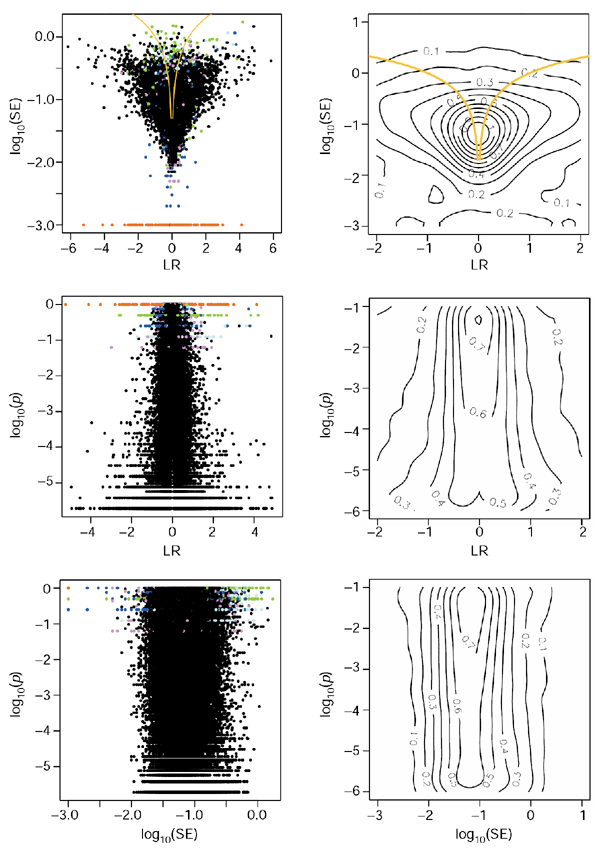
Relationships between the LR, SE and p measures for the PM-only scores. The right panels show contour plots of the densities raised to the power 0.2, so as to resolve structure in the low-density regions; the ranges of the right-hand panels were chosen to emphasize the most interesting features of the densities. The red, green, blue, cyan and magenta dots refer to N = 1, 2, 3, 4, 5 'good' cell pairs, respectively. Black dots have more than six good cell pairs. The yellow line in the top-left panel represents |LR| = SE, so that points below the line have signal-to-noise ratios > 1. The SE for the red dots (N = 1) is artificially set to 0.001 for plotting purposes; it should strictly be 0.

Figure 2.

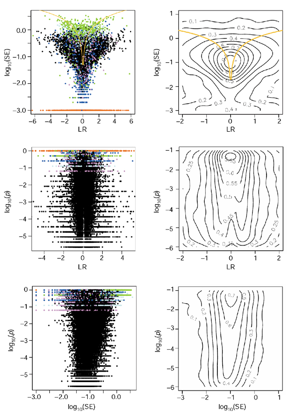
Relationships between the LR, SE and p measures for the PM-MM method. Description and colors as for Figure 1.

The difference in the log-ratios from the PM and PM-MM methods is illustrated in Figure 3. Although there is a branch with LR ~ 0 from the PM method when all p-values are considered, this branch rapidly disappears when focusing at smaller p-values only. Cases where the PM and PM-MM scores indicate regulation in opposite directions are virtually absent when p < 0.05. However, one can see a 'compression effect' in the scores from the PM method, shown by the edges with slope > 1 near the regions indicated by the arrows in the bottom right panel (this can also be seen by comparing the upper two contour plots of Figures 1 and 2). This compression probably reflects cross-hybridization effects that are not corrected for in the PM-only method. However, if one is more interested in finding significant changes than in the LR values themselves, the determining quantity is the LR value divided by the width of the local noise. Therefore, compression in the scale is not dramatic as long as the noise envelope also shrinks (see Discussion).

Figure 3.

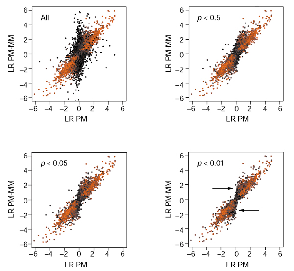
Comparison between the ratio scores from the PM-only and the PM-MM methods. Only genes with p-values (from the PM-MM method) smaller than indicated are plotted. The brightest red dots have the smallest p-values (around 10^-6), whereas black dots correspond to p = 1 (upper left panel) to p = 0.01 (lower right panel).

A comparison of the LR/SE (signal-to-noise ratio, SN) from both methods emphasizes the complementarity of both methods (Figure 4), as there is clearly a similar fraction of genes that have poor SN ratios (SN < 2) in one case but acceptable ratios in the other. These are found in the top-left and bottom-right quadrants defined by the horizontal and vertical blue lines.

Figure 4.

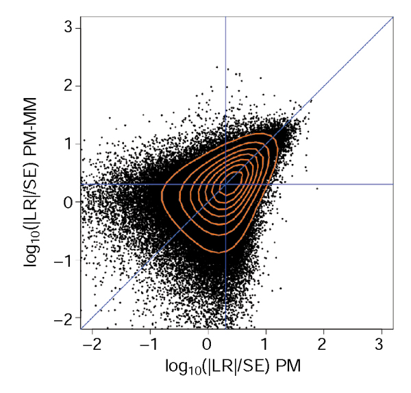
Comparison of the signal-to-noise ratios (SN) for the PM and PM-MM methods. Only genes with N_good > 4 in the PM-MM method are plotted. The red lines are contour lines and the blue lines denote the diagonal and SN values of 2 on either axis.

We have shown previously [11,12] using the same Mu11K dataset that our PM-only composite ratios lead to a reduction in variance, especially at low intensities, when compared to the Microarray Analysis Suite 3.2 available at that time.

Noise structure

In Figure 5 we show typical scatterplots with increasing levels of overall differential regulation, from duplicates to strong regulation (going from left to right). Although these particular data are from a subset of the Mu11KsubA chips used for Figures 1 and 2, our experience is that these are very typical of GeneChip hybridization data from numerous chip series. We shall always refer to duplicates as 'experiments' where the enzymatic steps (see Protocols in Materials and methods) in the target sample preparations have been performed independently. In ideal terms, the scatter cloud is thought of as consisting of two components: one is just noise from the enzymatic and hybridization steps affecting all the genes; the other reflects true sample differences. To illustrate this, we give three prototypical cases showing the data for the individual genes and the local variance regression lines (Figure 5). In these, the second component increases gradually from zero (left-most plot, duplicates), as visible in the quantile-quantile (QQ) plots in Figure 5b. The nearly straight left-most QQ plot indicates that variable LR/σ (η) closely follows a normal distribution. As the amount of true regulation increases, longer tails develop that depart from normal behavior.

Figure 5.

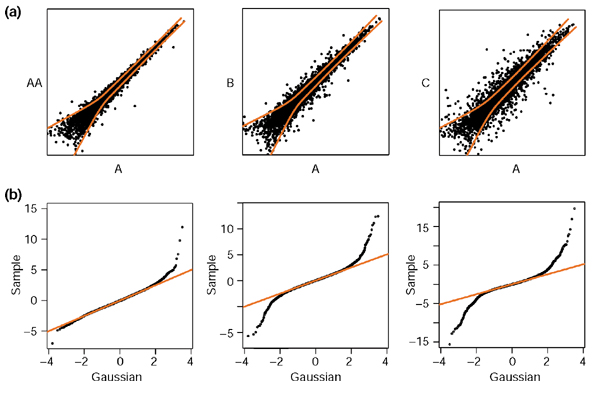
Scatterplot and quantile-quantile (QQ) plots. (a) Typical scatterplot showing increasing levels of differential regulation, together with the 2σ noise envelopes (red lines). There are three different conditions: A, B and C. AA is a duplicate of A. (b) Associated QQ plots of LR/σ (η). The data shown here were obtained using four out of the 12 Mu11KsubA chips used in Figures 1 and 2.

The fact that the noise component behaves as local log-normal distributions is not dictated by the choice of the variable LR/σ (η), on the contrary, it emerges as a rather pleasant feature of GeneChip experiments. In Figure 6, we demonstrate that this log-normality occurs very systematically: we show the two best and two worst (judged by the linearity of the QQ plots and the amount of outliers) from 40 human HG-U95A duplicates collected in a study of rheumatoid arthritis (see Materials and methods). The majority of the cases look closer to the first two examples; and the PM and PM-MM methods lead to equally good log-normal distributions overall. The mean and variation in the local SD for both the PM and PM-MM methods are shown in Figure 7 and reflect the characteristic contraction of the noise envelope with increasing coordinates along the diagonal. It is obvious that the PM noise envelope is thinner than that of the PM-MM at low intensity; on the other hand, both methods lead to comparable local σ in the 'flat' mid to high-intensity domains, where over half of the data lies. There, σ is approximately 0.15, so that 2σ corresponds to a ratio of 2^0.3 = 1.25, so 95% of repeated measurements would fall within a factor of 1.25 of their mean. Barring some artifact affecting large numbers of probes simultaneously, we would expect then that approximately 95% of the measurements in the mid- to high-intensity range are reproducible within a factor of around 1.25.

Figure 6.

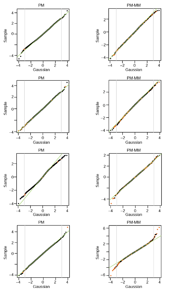
QQ plots of LRσ (η) versus normal distributions in replicate HG-U95A experiments. The examples shown are the two best and two worst of 40 replicates. The region between the gray lines contains 99.9% of the data. Red dots represent ratios with N_good < 5.

Figure 7.

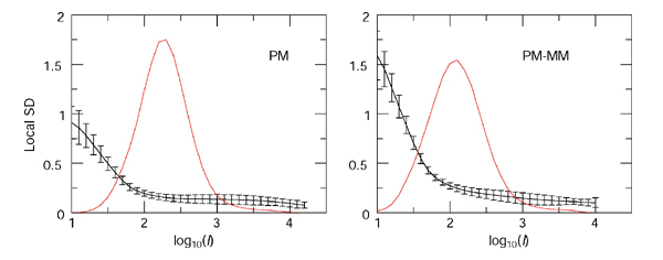
Intensity dependence of the noise envelope. SD of the log₂-ratios from 40 pairs of replicate HG-U95A experiments are in black. The errors represent the variation in local SD from the 40 replicates. The intensity I = (I_XI_Y) ^1/2 measures the coordinate along the diagonal of the scatterplots, and the red lines represent the density of the variable I in arbitrary units (but the same in both panels). Note that the mode of the PM-MM lies lower than that of the PM line.

Discussion

Our experience is that despite constant improvements, current incarnations of the arrays still behave fairly inhomogeneously as far as their PM and MM hybridization properties are concerned. This is probably the consequence of various sequence-dependent effects: first, the difference in stacking energies of single-stranded snippets between the PM and the MM sequences can easily be in the range of the gain in binding energies; second, there are certainly kinetic effects as the hybridizations are not carried to complete equilibrium; and third, there is always the possibility of sequence-dependent synthesis efficiencies. The wide range of probe set behavior is best seen in the SN ratios in Figure 4. For these reasons, we believe that a safe way to proceed is to integrate the results from both PM-only and PM-MM methods. For instance, considering the intersection (or union) of genes predicted by either method would minimize the false-positive (or false-negative) rates. In addition, there seems to be a significant variation in the hybridization properties across different chip series, as can be observed from simple statistics on the number of probe pairs with MM hybridizing better than PM (see Results). The superiority of the yeast chip mentioned above may of course be related to the relative simplicity of the yeast genome compared to that of the higher organisms.

Another point worth mentioning is that the values of the ratio scores may deviate from the real mRNA concentration ratios in some intensity regimes as the result of various effects such as non-linearities in the probes' binding affinities. Evidence concerning this matter has recently been reported [13]. This emphasizes the main point of our work, namely the importance of measuring differential expression relative to the local noise; only then can we decide whether a given ratio score can be considered as indicating true regulation or not.

Finally, the question of handling significance across replicated experiments is a second step to be built on top of the analysis presented above. The most reasonable approach would be to follow [7], namely to consider the t-statistics of the expression ratios across the samples. However, one would also want to weight the average according to the noise content in each of the samples, in a manner similar to that discussed in [8].

Materials and methods

Datasets and protocols

We briefly describe here the two datasets presented, and what we refer to in the text as the 'enzymatic steps'.

Mul IKsubA chips hybridized to adult mouse brain extracts

All six brain regions were obtained from adult (2-3-month-old) CD-1 mice. Dissections were carried out in ice-cold buffer, and tissues were immediately frozen with liquid nitrogen. Total RNA was isolated. Poly (A)⁺ RNA was then isolated with magnetic oligo-dT beads. For each brain region, 1 μg poly(A)⁺ RNA was converted to double-stranded T7 cDNA. Labeled cRNAs were produced from the double-stranded cDNA libraries and hybridized to chips according to the Affymetrix protocol, including the antibody-amplification step. All hybridizations were carried out in duplicate.

HG-U95A chips hybridized to human blood extracts

The same protocol was used, except that no poly(A) isolation was done before the conversion to cDNA.

Regression of the log-ratios, SE

To compute expression ratios for genes measured in two separate arrays, let (x_i, y_i) denote the brightness measurements for one probe set (the index i ranges from 1 to the number of probe pairs for the particular probe set, 14-20 depending on the chip series) taken in the two different hybridization arrays X and Y. We investigate both cases in which the intensities (x_i, y_i) are either the intensities of the background-subtracted PM cells or the PM-MM values (which need no background correction). Only N_good 'good' probe pairs are retained for determining the ratio and associated quantities. We discard probes that are saturated in both X and Y, or probe pairs such that PM-MM < 3 or PM < 3 in both X or Y. Here, corresponds to the standard deviation of the fluctuations in the background intensity. Not considering such probes prevents contamination of the ratio estimates from noisy low-intensity probes. After identifying the probe pairs allowed into the analysis, the differential expression score LR for the gene in question is obtained from a LTS robust regression of LR_i = log₂(x_i/y_i) to an intercept = LR. LTS regression corresponds to minimizing:

the sum of the Ns smallest squared residuals [14,15]. We used the default Ns = (N_good/2) + 1 and this parameter can be adjusted in our scripts; however, we found no evidence for changing the default. An estimate of the standard error (SE) for is given by SE = . Composite absolute intensities for the gene in each experiment can be obtained via geometric means of the (x_i, y_i) probes kept in the LTS regression, however, these are only indicative measures as the method was designed primarily for expression ratios.

Wilcoxon statistics, number of cells used

In addition to the SE, which reports a quantitative estimate of the error in the log-ratio measurement, it is also instructive to report a p-value from a paired Wilcoxon rank sign test of the LR_i values. Casually speaking, this value is related to the portion of the probes indicating gene regulation in the same direction: the theoretical minimum p-value, p_min, is achieved when all probe ratios agree on the same direction of regulation. Moreover, the test is non-parametric as it is operating in rank space, and p therefore also incorporates information about the number of probe pairs used (N_good). Namely, the Wilcoxon p-value has a lower bound that decreases with increasing sample size. For instance p_min = 1/4 for N_good = 3 and 1/8 for N_good = 4, so that small p scores can only be reached when enough probes are used. However, the converse is not true, as a gene that is not differentially expressed can have a p-value that is close to 1 even if all the probe pairs are 'good' in the above sense.

Our method does not primarily aim at quantifying the presence or absence of a gene in a particular sample. Nevertheless, we report the number of probes (N_above) with intensity larger than 3_eff (_eff = for the PM-MM case) for both samples X and Y. Using enough data, one could compute a probability of presence depending on N_above, and it is likely that this calibration would be dependent on the chip series.

Normalization and noise characterization

The measures described above are all single-gene properties; they can be computed when given just the intensities gathered for a single gene. In contrast, correcting for systematic trends (also called 'data massage') and more important, classifying expression ratios according to their significance, requires measures that involve the entire gene population on the arrays. We stress that these techniques are meaningful only when the number of genes probed is sufficiently large, and under the assumption that a large fraction of them does not show differential regulation between the two tested samples. These requirements are usually met in GeneChip experiments. Normalization aims at correcting for systematic trends (that is, bias as a result of dye efficiencies and amplification, sample concentration, photodetector efficiency) so as to make a collection of arrays directly comparable. One must distinguish global from local normalization: in the first, the intensities of all the probes on the array are scaled by a constant factor; in the second, the normalization factor can be intensity dependent. Local normalization techniques are mostly discussed in the context of cDNA arrays [16,17], where the intensity dependence can be severe. HDONAs suffer less from 'bent' noise structures; nevertheless, local normalization has also been introduced for them [18,19]. Although attractive, local normalization should not be applied blindly as it can hide real failures in the data and create its own artifacts. Our approach to normalization is based on centering the log-ratio distribution either globally, or locally as in [16]. For the data presented in the Results section, local normalization was used; however, our scripts allow a choice between the local and global schemes (see Additional data files for scripts). We always normalize an array with respect to another one, and we found it more accurate to do so at the gene rather than the probe level (we normalize the composite ratio scores a posteriori instead of normalizing the raw probe intensities).

Turning to the noise structure, significance of regulation is quantified from a local robust regression () of the variable LR² versus 77, where LR = log(I_X/I_Y) is the log-ratio of the intensities and = log(I_XI_Y)/2 is half the log-product. I_X and I_Y denote the locally normalized intensities of the genes in channels X and Y. We should emphasize that estimating the local variance in this manner only makes sense after the arrays have been locally normalized. The function () then quantifies the local log-ratio variance, so that the local SD is given by () = . We used the R routine loess for the fitting [15]. The justification for using the local SD as a criterion for significance relies upon the empirical fact that the variable LR/() follows a good normal distribution in the case of replicate (pure noise) experiments (see Figure 6). The significance of a ratio score can therefore be assessed using the value LR/SD; that is, a value LR/SD = 2 implies that the null hypothesis that the gene is not regulated can be rejected with a 95% confidence level.

We finally comment on the precise differences between our approach and that in [8]. First, we found no evidence for the inclusion of an additive term in linear coordinates. Judging by the data, the noise structure is very well captured by an effective multiplicative model (see Results). Second, the multiplicative noise component is estimated in logarithmic coordinates instead of linear, and after a local normalization. Finally, we estimate the local scale in the noise by an empirical robust fit of the local variance, with no a priori model. While it would be satisfactory to have a physical model describing the noise, our experience is that it is very hard to formulate one that accounts for the observed structure in all cases.

Additional data files

Scripts for converting between file types are available with this article (cdf2psc, cel2ratios, cel2raw, raw2pcel; see explanatory file for more details) and at the authors' website [20].

Supplementary Material

Additional data file 1

cdf2psc: converts a .cdf file into a .psc file.

Additional data file 2

cel2ratios: converts two .PCEL files into ratios.

Additional data file 3

cel2raw: converts .CEL files into .RAW files.

Additional data file 4

raw2pcel: estimates background and so on.

Additional data file 5

Explanatory file

A previous version of this manuscript was made available before peer review at http://genomebiology.com/2001/3/1/preprint/0001/

References

- Chee M, Yang R, Hubbell E, Berno A, Huang XC, Stern D, Winkler J, Lockhart DJ, Morris MS, Fodor SP. Accessing genetic information with high-density DNA arrays. Science. 1996;274:610–614. doi: 10.1126/science.274.5287.610. [DOI] [PubMed] [Google Scholar]
- Lipshutz RJ, Fodor SP, Gingeras TR, Lockhart DJ. High density synthetic oligonucleotide arrays. Nat Genet. 1999;21:20–24. doi: 10.1038/4447. [DOI] [PubMed] [Google Scholar]
- Lockhart DJ, Winzeler EA. Genomics, gene expression and DNA arrays. Nature. 2000;405:827–836. doi: 10.1038/35015701. [DOI] [PubMed] [Google Scholar]
- Kerr MK, Martin M, Churchill GA. Analysis of variance for gene expression microarray data. J Comput Biol. 2000;7:819–837. doi: 10.1089/10665270050514954. [DOI] [PubMed] [Google Scholar]
- Newton MA, Kendziorski CM, Richmond CS, Blattner FR, Tsui KW. On differential variability of expression ratios: improving statistical inference about gene expression changes from microarray data. J Comput Biol. 2001;8:37–52. doi: 10.1089/106652701300099074. [DOI] [PubMed] [Google Scholar]
- Tusher VG, Tibshirani R, Chu G. Significance analysis of microarrays applied to the ionizing radiation response. Proc Natl Acad Sci USA. 2001;98:5116–5121. doi: 10.1073/pnas.091062498. [DOI] [PMC free article] [PubMed] [Google Scholar]
- Speed group microarray page: statistical methods for identifying differentially expressed genes in replicated cDNA microarray experiments http://www.stat.berkeley.edu/users/terry/zarray/Html/matt.html
- Hughes TR, Marton MJ, Jones AR, Roberts CJ, Stoughton R, Armour CD, Bennett HA, Coffey E, Dai H, He YD, et al. Functional discovery via a compendium of expression profiles. Cell. 2000;102:109–126. doi: 10.1016/s0092-8674(00)00015-5. [DOI] [PubMed] [Google Scholar]
- Li C, Wong WH. Model-based analysis of oligonucleotide arrays: expression index computation and outlier detection. Proc Natl Acad Sci USA. 2001;98:31–36. doi: 10.1073/pnas.011404098. [DOI] [PMC free article] [PubMed] [Google Scholar]
- Li C, Wong WH. Model-based analysis of oligonucleotide arrays: model validation, design issues and standard error application. Genome Biol. 2001;2:research0032.1–0032.11. doi: 10.1186/gb-2001-2-8-research0032. [DOI] [PMC free article] [PubMed] [Google Scholar]
- Naef F, Lim DA, Patil N, Magnasco M. Proc DIMACS Workshop on Analysis of Gene Expression Data. American Mathematical Society; 2002. From features to expression: high-density oligonucleotide arrays analysis revisted. [Google Scholar]
- DNA hybridization to matched templates: a chip study http://xxx.lanl.gov/abs/physics/0111199 [DOI] [PubMed]
- Chudin E, Walker R, Kosaka A, Wu SX, Rabert D, Chang TK, Kreder DE. Assessment of the relationship between signal intensities and transcript concentration for Affymetrix GeneChip® arrays. Genome Biol. 2002;3:research0005.1–0005.10. doi: 10.1186/gb-2001-3-1-research0005. [DOI] [PMC free article] [PubMed] [Google Scholar]
- Rousseew PJ, Leroy AM. Robust Regression and Outlier Detection. New York: Wiley. 1987.
- Ihaka R, Gentleman R. A language for data analysis and graphics. J Comput Graph Stat. 1996;5:299–314. [Google Scholar]
- Tseng GC, Oh MK, Rohlin L, Liao JC, Wong WH. Issues in cDNA microarray analysis: quality filtering, channel normalization, models of variations and assessment of gene effects. Nucleic Acids Res. 2001;29:2549–2557. doi: 10.1093/nar/29.12.2549. [DOI] [PMC free article] [PubMed] [Google Scholar]
- Speed group microarray page: normalization for cDNA microarray data http://oz.berkeley.edu/users/terry/zarray/Html/normspie.html
- Schadt EE, Li C, Su C, Wong WH. Analyzing high-density oligonucleotide gene expression array data. J Cell Biochem. 2000;80:192–202. [PubMed] [Google Scholar]
- Hill AA, Brown EL, Whitley MZ, Tucker-Kellog G, Hunter CP, Slonim DK. Evaluation of normalization procedures for oligonucleotide array data based on spiked cRNA controls. Genome Biol. 2001;2:research0055.1–0055.13. doi: 10.1186/gb-2001-2-12-research0055. [DOI] [PMC free article] [PubMed] [Google Scholar]
- Scripts associated with this paper http://asterion.rockefeller.edu/felix/Affyscripts
Associated Data
This section collects any data citations, data availability statements, or supplementary materials included in this article.
Supplementary Materials