Search and match across spatial omics samples at single-cell resolution

Abstract

Spatial omics technologies characterize tissue molecular properties with spatial information, but integrating and comparing spatial data across different technologies and modalities is challenging. A comparative analysis tool that can search, match and visualize both similarities and differences of molecular features in space across multiple samples is lacking. To address this, we introduce CAST (cross-sample alignment of spatial omics), a deep graph neural network-based method enabling spatial-to-spatial searching and matching at the single-cell level. CAST aligns tissues based on intrinsic similarities of spatial molecular features and reconstructs spatially resolved single-cell multi-omic profiles. CAST further allows spatially resolved differential analysis ΔAnalysis) to pinpoint and visualize disease-associated molecular pathways and cell–cell interactions and single-cell relative translational efficiency profiling to reveal variations in translational control across cell types and regions. CAST serves as an integrative framework for seamless single-cell spatial data searching and matching across technologies, modalities and sample conditions.

Spatial omics technologies enable direct profiling of gene expression and molecular cell types in intact tissues, organs^1–5 and across different modalities such as epigenomes⁶, translatomes⁷ and proteomes⁸. Analogous to atlas integration for single-cell omics, an ideal spatial integration tool for spatial omics should serve as a search engine and comparative analyzer to search, match and visualize the similarity and differences among samples. Meanwhile, it should work robustly when dealing with vast numbers of cells, spanning various conditions and modalities. As spatial transcriptomics data contains much richer information than traditional staining (for example 4’,6-diamidino-2-phenylindole (DAPI), hematoxylin and eosin (H&E) and Nissl), transcriptomics-based registration may be more advantageous and accurate than established image-based registration. Additionally, image-based registration may be compromised when the staining method, quality, resolution or sample size are different between the training models and query images; however, current transcriptomics-based spatial alignment methods⁹ can only handle small-scale, low-resolution and highly similar datasets collected from the same wet-lab technology. On the other hand, image registration methods typically require landmark annotations and struggle with discrepancies in image properties. Moreover, effective full-stack spatial integration methods that allow accurate search-and-match of spatial omics data across technologies, modalities and conditions have not been achieved yet.

To address this, we introduce CAST (cross-sample alignment of spatial omics data) for searching, matching and visualizing the similarities and differences across spatial omics datasets. CAST is composed of three modules: CAST Mark, CAST Stack and CAST Projection (Fig. 1a,b). It leverages deep graph neural networks (GNNs) and physical alignment to harmonize spatial multi-omics data at the single-cell level while preserving cellular proximity in tissue niches. CAST can detect fine-grained common spatial features, perform robust physical alignment and integrate samples of different spatial modalities, resolutions and sizes. It is applicable across various low- and high-resolution spatial technologies (Visium, STARmap⁵, MERFISH², RIBOmap⁷, Slide-seq³ and Stereo-seq⁴) and can accurately match spatial samples of different sizes and gene numbers based on their inherent tissue properties, without supervision nor manual annotation of the region of interest (ROI).

Fig. 1 |. Schematic overview of CAST.

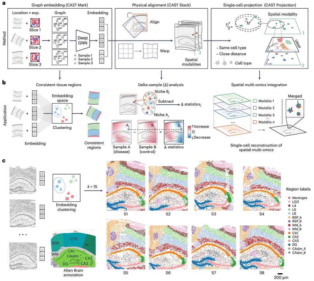
a, The principles of the three modules in CAST. b, The applications enabled by the three modules of CAST. c, CAST Mark identifies consistent regions across multiple samples. The k-means (k = 15) clustering results of the graph embedding generated by CAST Mark across the samples S1–S8 in the STARmap PLUS dataset (Supplementary Table 2), in comparison with the Allen Brain Atlas^17,18. Different colors in the cells indicate the different clusters of the graph embedding. UMAP, Uniform Manifold Approximation and Projection; CTX, cerebral cortex; RSP, retrosplenial area; WM, white matter; DG, dentate gyrus; CAslm, CA stratum lacunosum-moleculare; CA1–3, hippocampal CA1–3 region; L2/3, L4, L5, L6, cortical layers 2/3, 4, 5 and 6, respectively.

Results

CAST Mark captures common spatial signatures across samples

Representing tissue samples using graphs⁸ shows the potential to overcome the inconsistent physical coordinates caused by different magnification, individual variation and experimental batch effects. GNNs operate on graphs and have been recently used to learn representations of tissue organization of spatially resolved transcriptomics measurements^10–15; however, traditional GNN architectures suffer from the over-smoothing problem that limits the depth of the network, raising doubts about their capability to capture large-scale continuities in tissue biology¹⁴. In addition, the traditional GNN architectures cannot identify the common spatial features across the samples in an unsupervised manner. To address these limitations, we created CAST Mark, a GNN model equipped with (1) graph convolutional network via initial residual and identity mapping (GCNII) layers, which were designed to overcome the over-smoothing problem¹⁶, making the GNN learnable with a nine-layer depth; and (2) a self-supervised learning objective (Extended Data Fig. 1a and Methods). By using the GCNII layers, CAST Mark overcomes the limited depth in a traditional GNN model and now has a large receptive field that enables unsupervised learning of spatial features using only single-cell gene expression profiles and physical cell coordinates as input, without requiring cell-type or tissue-region annotations. We further confirmed the technical advancement and performance of the CAST Mark model by parameter sensitivity and ablation studies (Supplementary Figs. 1–3 and Supplementary Information).

To evaluate the performance of the CAST Mark in learning the graph representations of cell locations across different samples, we first applied CAST Mark to a synthetic dataset consisting of one ground-truth sample (S1) from a STARmap PLUS dataset⁵ and a simulated sample (S1′) generated by applying random noise, feature dropouts and global tissue distortion to sample S1 (Extended Data Fig. 1b and Methods). Each cell in the simulated sample S1′ has a one-to-one ground-truth partner cell in sample S1. We performed k-means clustering on the graph embedding to examine whether CAST Mark could retain the shared spatial information between S1 and S1′. Although the graph structures of S1 and S1′ are different due to added random noise, the regional patterns are consistent across samples in both the physical space (Extended Data Fig. 1c) and the graph embedding space (Extended Data Fig. 1d). These observations are confirmed by quantitative analysis, where 20 clusters show a high adjusted Rand index (ARI) (averaged ARI = 0.79, ten replicates) and on average 90% of cells in S1′ belong to the same clusters as its ground-truth partners in S1 (Extended Data Fig. 1e). Notably, even when increasing the number of clusters k to 100, the clustering results still show a considerable cross-sample consistency both by visual inspection and quantification (Extended Data Fig. 1e,f; averaged ARI = 0.47, averaged consistent cell percentage of 56%). Furthermore, despite different clustering parameters (10–100), each cell is still physically adjacent (average distance of 6.95 μm, smaller than the typical size of a cell) to the correct clusters (Extended Data Fig. 1g), suggesting the robust performance of CAST Mark despite sample variability.

Benchmarks of the CAST Mark GNN (Supplementary Table 1) show superior performance than existing methods in terms of resolution and contiguity in sample S1 (Extended Data Fig. 1h) and a mouse half-brain coronal sample containing ~60,000 cells (Extended Data Fig. 1i).

Encouraged by the cross-sample consistency of CAST Mark graph embedding trained on the synthetic dataset, we next examined whether CAST Mark could achieve consistent label-free segmentation with real biological samples. We applied CAST Mark to the 2,766-gene STARmap PLUS dataset⁵ composed of eight coronal brain slices near the hippocampus region (slices S1–S8) from multiple mice with different conditions, ages and strains (Supplementary Table 2). K-means clustering (k = 15) yielded consistent tissue-region identification across the eight samples (Fig. 1c), which agreed well with existing knowledge of mouse brain anatomy^17,18. We further tested an extremely high clustering resolution by 100-class k-means clustering (k = 100) and the results still showed remarkable consistency across the eight samples (Extended Data Fig. 2a), suggesting the ability of the CAST Mark learning scheme in resolving fine tissue architectures consistently across all samples, although the biological meaning of those fine clusters warrants further investigation.

Notably, the consistent patterns of gene expression and cell-type abundance (Extended Data Fig. 2b–d and Supplementary Table 3) across the eight samples strongly support that CAST can robustly identify the concordant and biologically meaningful spatial features across different samples with biological and individual variations, which are further used as a foundation for sample alignment.

CAST Stack performs robust physical alignment across samples

As the cytoarchitecture of tissue samples falls on a spectrum between completely stereotypical to random, an ideal alignment method should meet the following requirements: (1) robust correction of local differences in batches, conditions, tissue morphology and experimental technologies; and (2) preservation of cellular organization inside the tissue.

As CAST Mark is capable of generating common graph embeddings for cells across multiple samples, we hypothesize that the similarity of cellular graph embeddings reflects the physical proximity of the cells in tissues and thus can be used to physically register one query tissue sample to the reference sample. To test this, we used the synthetic sample (S1′) as the query and the ground-truth sample (S1) as the reference. Given one cell in the query sample, we calculated the Pearson correlation (r) between the graph embeddings of the query cell and all the cells in the reference sample. We found that ground-truth pairs between S1 and S1′ show a strong correlation (average r = 0.97; Fig. 2a), while randomly chosen cell pairs show little correlation (average r = 0.04; Fig. 2a). And only its ground-truth paired cell and the closest randomly paired cells (top 0.1%) to this ground-truth pair exhibited a strong Pearson correlation with the query cell (Fig. 2b). When plotted in the physical space, cells in the reference sample that are highly correlated with the query cell are predominantly localized around the ground-truth reference cell, especially within the same tissue region (Fig. 2c and Extended Data Fig. 3a).

Fig. 2 |. CAST Stack automatically aligns tissue samples from biological replicates.

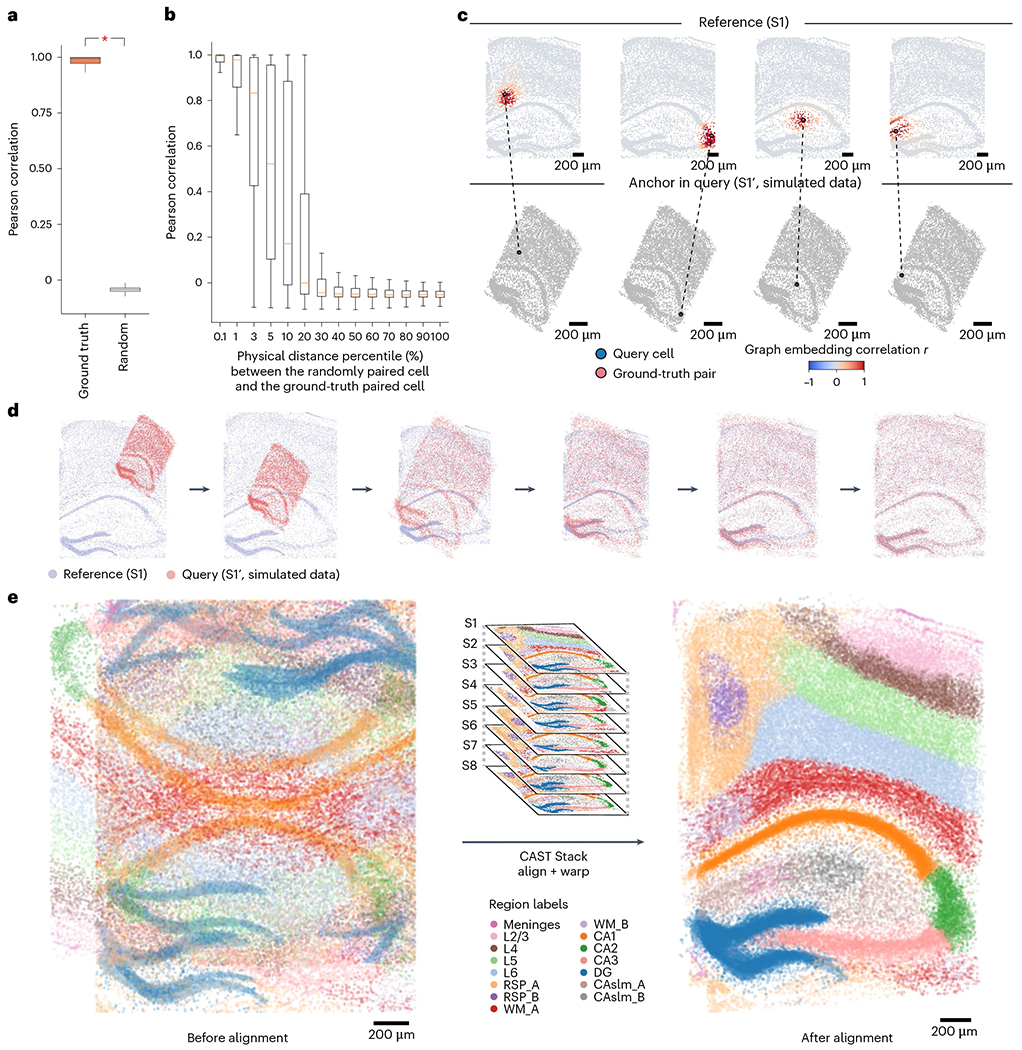
a, The boxplot shows a significantly higher (one-way analysis of variance (ANOVA); P < 2.2 × 10⁻¹⁶) Pearson correlation of graph embedding of the ground-truth cell pairs (ground-truth, mean of 0.97, n = 8,789) than the ones in the random distribution (random, mean of 0.04, n = 8,789) between samples S1′ and S1. b, For each query cell in the query sample (S1′), the CAST Mark embedding Pearson correlation (r) between this query cell and randomly paired cells as well as its ground-truth pair in the reference sample S1 is calculated. The horizontal axis indicates the distance percentile (%) of the randomly paired cell to the ground-truth pair. For example, 0.1 indicates the percentile group 0–0.1%, whereas 100 indicates the percentile group 90–100%. In the boxplots (a,b), the middle line indicates the median; and the first and third quartiles are shown by the lower and upper lines, respectively; the upper and lower whiskers extend to values not exceeding 1.5 × interquartile range (IQR). The number of samples is detailed in the Methods. c, Given the query cell in the query sample (simulated dataset S1′), the cells in the reference sample (S1) are colored by Pearson correlation of the graph embedding between the reference cells and the given query cell. d, Schematic demonstration of the CAST Stack alignment process. The alignment process of the simulated dataset S1′ (query sample) and S1 (reference sample) is visualized. e, CAST Stack aligns eight samples (S1–S8) into a consistent physical coordinate system. Cells are colored by tissue region labels generated by CAST Mark, the same as is shown in Fig. 1c.

Based on this observation, we concluded that the cross-sample correlations of cell pairs could predict their probable match of tissue locations. However, due to the inherent anatomical diversity across samples, we would lose the cell organization if we simply assigned each query cell to the position with the highest similarity of the graph embedding. Therefore, we designed a gradient descent (GD)-based approach to minimize overall cell location differences while preserving tissue structure during alignment transformations, by maximizing the sum of similarity between each query cell and its nearest reference cell (Methods). Instead of building alignment by satisfying every cell at its optimum, CAST Stack prioritizes preserving biologically meaningful tissue structure and avoids local minimums possibly derived from stochastic sample variations. We designed the CAST Stack alignment as a two-phase process. During the first phase, only global affine transformation is allowed. After affine transformation roughly aligns the samples, in the second phase, CAST Stack utilizes B-spline free-form deformation (FFD), a powerful constrained nonlinear warping approach, to handle local morphological differences among tissue samples.

We then applied this soft registration strategy to the S1′–S1 query–reference pair (Fig. 2d). Despite large structural and morphological differences introduced in S1′, the two samples were accurately aligned according to the high spatial correlations (Pearson r of graph embeddings between cells, same below unless otherwise stated) between the query cells and their nearest neighbors in the reference slice (Extended Data Fig. 3b). After the soft registration, the physical distances between the ground-truth pairs (average distance of 38 μm; Extended Data Fig. 3c) are significantly smaller than the random pairs (average distance of 1,133 μm; Extended Data Fig. 3c), confirming that CAST can precisely align two different slices into a consistent physical coordinate system.

Next, we applied CAST Stack to the eight hippocampal brain samples (S1–S8) from different mice with varied tissue morphologies, ages and conditions⁵. We selected S1 as the reference slice and subsequently aligned S2–S8 to S1 using CAST Stack. Similar to the S1′–S1 query–reference pair, cells from S2–S8 have the highest spatial correlation with cells from S1 at the corresponding tissue locations, especially within the same cluster of graph embeddings from CAST Mark (Extended Data Fig. 3d). After alignment, all the cells in the query samples (S2–S8) are transformed to the same physical coordinate system defined by the S1 reference (Fig. 2e and Extended Data Fig. 3e). The high correlation between the query cells with its closest physical neighbor cell in the S1 reference (Extended Data Fig. 3e) suggests that CAST Stack properly aligns each sample through soft registration while preserving the cellular organization of the tissues.

To demonstrate the wide utility of CAST, we applied CAST on different spatial technologies, such as Visium, Stereo-seq⁴, MERFISH¹⁹ and Slide-seq²⁰. Samples with similar size can be efficiently aligned not just within a single technology but also across multiple different technologies (Fig. 3a, Extended Data Fig. 4a–d and Supplementary Table 4). Notably, samples from three different technologies can be aligned into one shared physical coordinate system (Fig. 3a). Additionally, we also tested the performance of CAST Mark and CAST Stack with limited gene panels. CAST successfully aligned two STARmap samples collected with a small panel of 64 genes (S64_1 and S64_2; Extended Data Fig. 4e). CAST also aligned samples with drastically different gene panels with limited overlapping genes, showcased by the successful alignment of a 64-gene sample to a 2,766-gene sample (S64_1 and S1; Fig. 3b).

Fig. 3 |. CAST aligns tissue samples across spatial technologies regardless of different tissue areas and gene panel sizes.

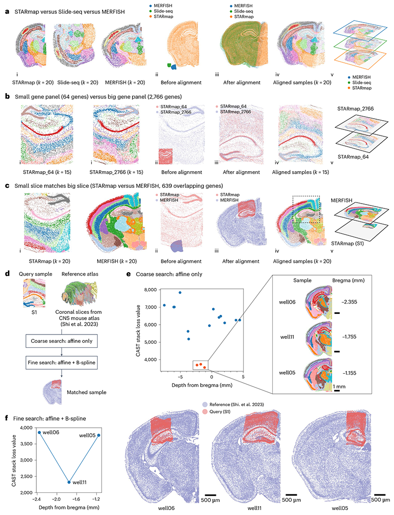
a, CAST integrates three samples of Slide-seq²⁰, MERFISH¹⁹ and STARmap (STARmap_mouse1 (ref. 7)), respectively, generating a shared physical coordinate system. (i) Thejoint k-means clustering results of CAST Mark graph embeddings of STARmap (left), Slide-seq (middle) and MERFISH (right), colored by joint clusters. (ii,iii) Spatial coordinates of the samples before (ii) and after (iii) alignment. (iv,v) Aligned samples colored by joint k-means clustering results of the graph embedding (two-dimensional visualization (iv) and three-dimensional visualization (v)). b, CAST Stack aligns the samples with different gene panels and different probe designs. STARmap_64 (left) is S64_1 (ref. 5) (Supplementary Table 2) and STARmap_2766 (right) is S1. The two samples share only 64 genes. The panel order is the same as in a. c, CAST automatically searches and matches a small slice (left) to a big slice (right) across technologies at high spatial resolution (STARmap (S1) versus MERFISH¹⁹). The panel order is the same as in a. d, The flowchart shows the two-step strategy to align query sample S1 (same as Fig. 1c for visualization) to the reference atlas. e, The loss value (the sum of the adjusted Pearson distance) is used as a score to screen for possible hits (only perform affine transformation). A score funnel is formed around the ground-truth slicing depth (calculated as the distance to bregma), indicating the possible matching tissue slices are sliced at the depth range of −1.155 mm to −2.355 mm. f, The complete CAST Stack alignment with optimized parameters were performed among the screened hits to identify the most matching tissue locations of the query sample. Final CAST Stack alignment results (right) are shown along with loss values (left). The aligned result of well11 is also displayed in d.

Notably, CAST shows the capability to precisely locate a small, truncated tissue section (hippocampus and partial cortical region) with larger half-brain slices measured by different spatial technologies and size (STARmap, MERFISH and Slide-seq), without manually specifying the ROI nor annotating landmarks (Fig. 3c, Extended Data Fig. 4f,g and Supplementary Video 1).

Given the ability of CAST to precisely match partially overlapping tissue locations between small and large tissue slices, we explored its potential to search one query sample against large reference atlas datasets/databases. We utilized the STARmap S1 sample, a subset of mouse coronal brain section, to query against a mouse central nervous system spatial transcriptomics atlas²¹ (2,766 versus 1,022, with 931 overlapping genes, Fig. 3d). Each section in the atlas is annotated with the distance to bregma that describes the relative depth along the anterior–posterior axis of the brain, which was obtained through physical registration with the Allen Mouse Brain Common Coordinate Framework (CCFv3) (ref. 18). These coronal brain sections represent different tissue morphology and anatomy of the mouse brain and could serve as a reference atlas for future query applications. We conducted the atlas query in the following two steps (Fig. 3d). First, we conducted a coarse search by using CAST Stack allowing only affine transformation to align the query sample S1 to all coronal sections in our reference atlas using shared uniform parameters. We reasoned that for each depth in the reference atlas, this could allow for a quick search of the most similar tissue locations possible to place the query sample S1. We visualized loss values of CAST Stack (the sum of the adjusted Pearson distance) after alignment. From this initial screening run with the affine transformation, we identified three sections in the reference atlas with the lowest loss values, which indicates the highest similarity (Fig. 3e). The sections are located adjacent to each other (the distances to bregma are −1.155 mm, −1.755 mm, −2.355 mm, respectively) along the anterior–posterior axis. Second, we further conducted a fine search by applying the full CAST Stack with both affine and nonrigid B-spline transformation to find the best match between S1 and three hits from the coarse search phase (Fig. 3f; distance to bregma = −1.755 mm).

In addition to benchmarking the parameters and the computational efficiency (Supplementary Figs. 4 and 5), we compared CAST with the existing spatial alignment tool PASTE, which adopts optimal transport to perform only global affine transformation to align voxel-based spatial transcriptomics data⁹. PASTE successfully aligned the Visium datasets (Supplementary Fig. 6a,b) but failed to align single-cell-resolved transcriptomics datasets (S2–S8 with S1) (Supplementary Fig. 6c–e) or align the spatial datasets with a large number of cells or voxels (Supplementary Table 5).

Identifying disease/injury-associated spatial features

Traditional single-cell analysis workflows can be adapted to find significant differences between samples, such as cell-type abundance, differential gene expression and cell–cell interactions (CCIs) in the spatial transcriptomics data⁵; however, by preserving single-cell resolved spatial relationships, it is possible to interrogate the continuous spatial gradients of such differences in cellular neighborhoods across multiple samples with unified tissue coordinates²² (Fig. 4a). Here, enabled by the physical alignment of CAST Stack, we further introduce a new spatial omics analysis strategy, delta-sample analysis (ΔAnalysis; Methods), to uncover comparative spatial heterogeneity across tissue samples: (1) given a cell and a physical radius (R), we first defined a cell-centered neighborhood, termed the spatial niche; (2) we then analyzed the local difference of interrogated features between samples within R, such as cell abundance (ΔCell), gene expression (ΔExp), cell–cell adjacency (ΔCCA) and CCI (ΔCCI, for example ligand–receptor interactions), which can be visualized as spatial gradient maps (Fig. 4a); and (3) by aggregating the local Δ features of single cells throughout the replicates and samples, we conducted statistical analysis at a single-cell level to test whether there was a significant difference of spatially resolved features between samples.

Fig. 4 |. Delta-sample analysis detects disease-associated spatial features.

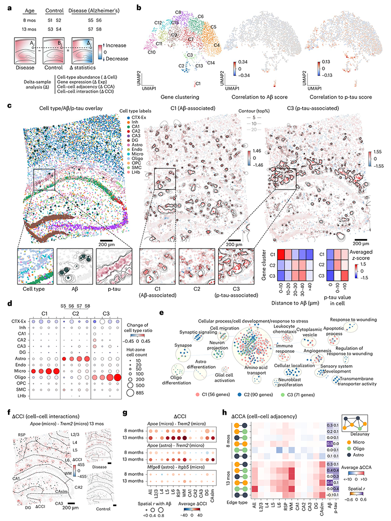
a, ΔAnalysis is performed to interrogate the spatial differences between different conditions (Supplementary Table 2). b, The UMAP of the ΔExp (R = 20 μm) spatial-pattern-based clustering results (left), paired with the Pearson correlation (r) of the ΔExp with the Aβ plaque score (middle) and p-tau score (right) across all disease samples. c, Cell type, Aβ plaque (dark green dots) and p-tau (pink) profile of S8 (left). Averaged ΔExp of C1 (middle) and C3 (right) genes paired with the contour lines (middle and right). The zoomed-in sections show the details of the cell type, Aβ plaque and p-tau in S8, as well as the averaged ΔExp (log₂_norm1e4) of C1, C2 and C3 genes in the same ROI. The size of the dark green dot indicates the area of Aβ plaques. The following heatmaps show the averaged scaled ΔExp profile of three clusters within each cluster in different cell groups. The cells are grouped by their distances to the nearest Aβ plaque (left) and their tau values (right). Astro, astrocyte; CA1, CA1 excitatory neuron; CA2, CA2 excitatory neuron; CA3, CA3 excitatory neuron; CTX-Ex, cortex excitatory neuron; Endo, endothelial cell; Inh, inhibitory neuron; Micro, microglia; Oligo, oligodendrocyte; OPC, oligodendrocyte precursor cell; SMC, smooth muscle cell; LHb, lateral habenula. d, Dot plots show the difference in cell type ratios between the hot-zone of the C1, C2, C3 and their non-hot-zone groups. The dot size indicates the cell count number in the hot-zone. e, GO enrichment analysis of the C1–C3. f, The ΔCCI (R = 50 μm) pattern of the Apoe (Micro) - Trem2 (Micro) in the 13-month comparison (S8 – (S3 + S4)/2). The size of dark green dots shows Aβ plaque area. The dash lines indicate the different CAST Mark regions. g, The ΔCCI pattern of selected ligand–receptor pairs in different regions and comparisons. The dot size indicates the spatial correlation between ΔCCI and Aβ plaque. h, The average spatial correlation (Pearson r) between the ΔCCA (R = 50 μm) and the Aβ plaque score as well as p-tau scores (Methods) are displayed. The values of four combinations in each comparison are averaged (13-month comparison, S7 – S3, S7 – S4, S8 – S3 and S8 – S4; 8-month comparison, S5 – S1, S5 – S2, S6 – S1 and S6 – S2).

Next, we demonstrate ΔAnalysis on S1–S8, which are collected on four TauPS2APP Alzheimer’s disease (AD) mice and four age-matched wild-type mice (Fig. 4a).

To unbiasedly uncover the disease-associated loci, we first clustered the genes based on their similarity of ΔExp spatial profiles across all disease samples (Fig. 4b). We observed that gene clusters C1, C2 and C3 displayed relatively high correlation of ΔExp with the amyloid beta (Aβ) plaque and p-tau (Fig. 4b), which hinted that these gene modules may associate with AD. Next, we plotted the heterogenous ΔExp landscape of the C1–C3 as contour maps (Fig. 4c) and further defined the hot-zones as the loci with the highest differential expression of these gene clusters (Methods). Notably, the C1 hot-zone contained remarkable Aβ plaque enrichment (Fisher’s exact test and odds ratio: 13 months, 15.8 and 16.48, respectively; and 8 months, 10.87 and 16.63, respectively) and C1 genes were over-expressed in the cells close to the Aβ plaque (0–10 μm group; Fig. 4c, Extended Data Fig. 5a and Supplementary Table 6). In contrast, C3 hot-zone was enriched with p-tau (Fisher’s exact test and odds ratio: 13 months, 1.98 and 5.78 months, respectively; and 8 months, 3.43 and 2.56, respectively) and C3 genes were upregulated in the cells with high p-tau values (p-tau value > 10 group; Fig. 4c, Extended Data Fig. 5b and Supplementary Table 6). The C1 and C3 hot-zones were also enriched with microglia and oligodendrocytes, respectively (Fig. 4d). Also, the C2 hot-zone was mainly enriched with astrocytes, whose expression was upregulated in the 20–40 μm vicinity of Aβ plaques and spatially associated with the immediate intensity group of p-tau. Meanwhile, the Gene Ontology (GO) analysis of these three gene modules (Fig. 4e) showed that these genes are related to cell migration (GO:0016477; shared by C1, C2 and C3), apoptotic process (GO:0006915; unique to C1), regulation of response to wounding (GO:1903034; unique to C2) and regulation of oligodendrocyte differentiation (GO:0048713; unique to C3). Consistent with a previous publication⁵, these observations revealed the disease association of microglia, oligodendrocytes and astrocytes, which were further validated by the cell-type-specific ΔExp and ΔCell (Extended Data Fig. 5c–i, Supplementary Fig. 7 and Supplementary Information). We further investigated disease-associated CCA and CCIs²³, which revealed Aβ-plaque-associated changes of the glial cell adjacency network and ligand–receptor interactions (ligand Apoe in microglia or astrocytes–Trem2 receptor in microglia^24–27 and ligand Mfge8 in astrocyte–Itgb5 receptor in microglia²⁸) along disease progression (Fig. 4f–h and Extended Data Fig. 5c,j).

Beyond the disease versus control demonstration to delineate the spatial and temporal changes during disease progression, we next applied CAST and ΔAnalysis to the axolotl brain regeneration dataset profiled by Stereo-seq²⁹. This axolotl brain dataset contains coronal slices of the axolotl brain with experimentally introduced injuries on one hemisphere, while the other hemisphere remained intact and healthy as the control at different days post-injury (DPI) along the brain regeneration process. We performed CAST alignment to physically align the injured brain hemisphere to the healthy brain hemisphere within each sample (Extended Data Fig. 6a,b). Afterwards, the ΔAnalysis (radius of 100 in initial pixel units in the dataset, 43 μm as indicated by the scale bar in the initial study) was applied to each aligned sample to investigate the injury-associated spatial molecular patterns.

With the ΔCell analysis, we observed cell types with relatively decreased and increased cell counts in the injured region, such as the decreased Nptx⁺ lateral pallium excitatory neurons (nptxEX) and the increased reactive ependymoglial cells (reaEGC) at the 2DPI stage (Supplementary Fig. 8a), consistent with an initial report²⁹. Concordantly, the ΔExp screening also revealed the decreased Nptx1 (marker gene for nptxEX cells) and increased S100a10 (marker genes for reaEGCs) patterns in the lesion region of 2DPI stage. To systematically discover injury-associated gene programs, we next clustered the genes based on the spatial profiles of the ΔExp across all samples (Extended Data Fig. 6c,d). By screening averaged ΔExp profiles in each gene, we identified two gene clusters with increased gene expression (cluster 6 and 9). Furthermore, the averaged ΔExp of the two clusters showed a spatially confined expression pattern around lesion sites (Extended Data Fig. 6e). We thus annotated them as injury-associated genes for downstream analyses. Cluster 6 enriched with previously reported injury-associated genes, such as S100a10, Nes, Ctsl, Tnc, Gfap and Krt18, whereas cluster 9 contained lots of ribosomal genes, such as Rps2, Rps7 and Rps18. As reflected by the GO analysis (Extended Data Fig. 6f), cluster 6 and 9 genes are functionally enriched in ribosome biogenesis (GO:0042254; shared by cluster 6 and 9), regulation of apoptotic process (GO:0042981; unique to cluster 6) and regulation of RNA splicing (GO:0043484; unique to cluster 9), suggesting potential upregulated roles of post-transcriptional gene regulation, including translational control in tissue regeneration. In addition, we visualized a few examples of newly identified injury-associated genes, such as the galectin 1 gene Lgals1, actin-binding protein Tagln2, and ribosomal proteins Rps7 and Rps18, which displayed a strong increased pattern in the lesion region across all DPI time points (Supplementary Fig. 8b).

Overall, the spatial gradient obtained through our ΔAnalysis reveals the spatial heterogeneity of cell-type composition, gene expression and cell–cell communications in diseased or injured samples versus controls, which enables us to analyze disease pathology or regeneration process at a higher spatial resolution.

CAST Projection reconstructs spatial multi-omics datasets

Beyond performing ΔAnalyses, consistent spatial coordinates generated by CAST Stack further allow us to integrate samples with different spatial omic modalities. Here, we introduce CAST Projection, an unsupervised, label-free method to project single cells from query samples onto a reference sample toward spatially resolved single-cell multi-omics (Fig. 5a). To achieve this, it assigns single cells from the query samples to the reference sample with the closest physical location and the most similar gene expression profile (for example the same cell type and cell state). Specifically, we first conducted Combat³⁰ and Harmony³¹ (Methods) single-cell data integration of the query and reference samples across different omic modalities to generate a shared low-dimensional latent space, where cosine distance, a widely used metric in single-cell analysis^32–34, is used to measure the similarity of cells across modalities. Given one reference cell, CAST Projection then searches for the cell with the closest cosine distance from the query sample within a confined physical radius as the matched cell pair (Methods). With well-aligned samples from CAST Stack, we can easily project the cells from multiple query samples to a shared reference sample with identical tissue coordinates.

Fig. 5 |. CAST Projection enables single-cell integration of spatial omics data across multiple samples.

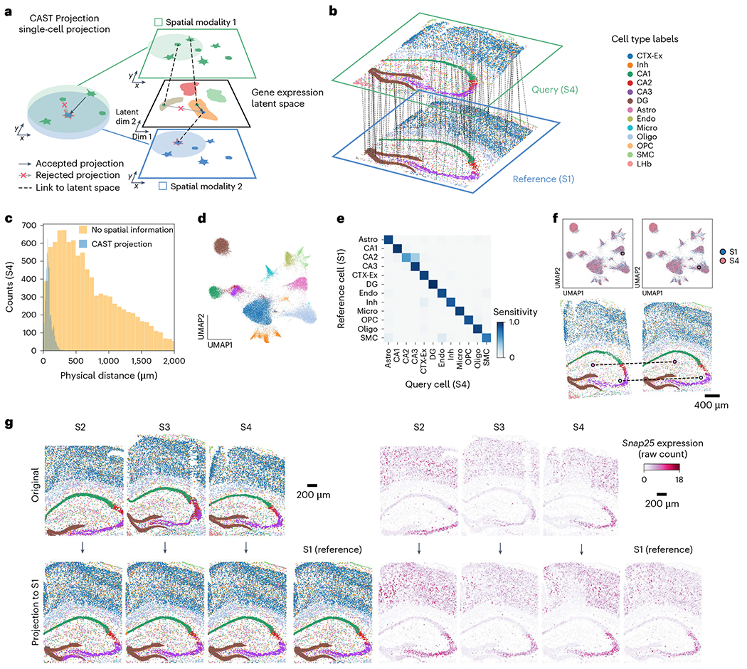
a, Strategy of the spatially and single-cell resolved cell assignment used by CAST Projection. b, Schematic for CAST Projection results. Dashed lines (100 randomly sampled assignment pairs for visualization) connect cells from the query sample (S4) with its destination cell in the reference sample (S1). Colors represent cell types. c, The distribution of the physical distances in the spatial single-cell projection of the S4 to S1. The blue is the CAST Projection strategy, while the yellow is the strategy that projects the query cell with the closest cosine distance to each reference cell without spatial constraints (same as Supplementary Fig. 9). d, UMAP of the batch-corrected latent space across S1–S4 samples (control samples). Colors follow figure legends in b. e, Confusion matrix of CAST Projection (S4 to S1, true positive rate of 0.91). To analyze cell types with an adequate sample size, we filtered out those that have fewer than ten cells in the reference sample. f, CAST Projection assignment examples from S4 (query sample, pink) to S1 (reference sample, blue) in the UMAP plot (top) and spatial coordinates (bottom; colors follow figure legends in b). g, CAST Projection reconstructs one sample with multiple datasets. Cells are colored by cell types (left) (colors follow figure legends in b); the Snap25 gene expression (raw count) profiles (right) in the original samples (top, S2–S4) and projected samples (bottom).

We first evaluated the performance of CAST Projection using four control samples (S1–S4). When performing projection from S4 (query) to S1 (reference) (Fig. 5b and Supplementary Video 2), the Euclidean distance of assigned cell pairs indicated that most of the cells in the query slice were assigned to the reference slice with small distances (median distance of 72 μm; Fig. 5c). Meanwhile, the cell types of reference cells were highly concordant with their assigned query cells, shown by the confusion matrix of cell type assignments (91% matched labels; Fig. 5d–f and Extended Data Fig. 7a), which further supports that CAST correctly projects single cells from one tissue slice to another with the accurate match of spatial location and gene expression profiles.

Using CAST Projection, we finally integrated four biological samples (S1–S4) into one spatial common coordinate framework (Extended Data Fig. 7b–d) in which every single cell consists of four gene expression profiles (Fig. 5g). Gene expression profiles showed consistent spatial patterns across S1–S4 before and after projection, such as Snap25 (Fig. 5g), Mobp and Tshz2 (Extended Data Fig. 7e). Notably, experimental flaws (for example tissue distortion, slice fracture and missing imaging tiles) in individual slices do not significantly harm the performance of CAST and can be well compensated for by aggregating information from multiple samples through the spatial and single-cell integration of the CAST Projection process (Fig. 5g and Extended Data Fig. 7e).

Next, we examined whether spatial constraints are necessary by comparing against an alternative projection strategy of matching query cells with each reference cell solely relying on single-cell cosine distance without spatial constraints (Fig. 5c and Supplementary Fig. 9). Although this strategy generated comparable results in terms of matching cell types, the projection plots and the physical distance histograms showed that the projections were much further away from the reasonable locations compared to the CAST Projection, pointing out the importance of the spatial constraints. Similarly, CAST Projection with spatial constraints outperformed existing single-cell-to-spatial integration tools, such as Tangram³⁵ and Cell2Location³⁶ (Supplementary Fig. 10a,b). Both demonstrations collectively suggest that direct spatial-to-spatial alignment may be closer to the ground truth for spatial multi-omic integration in comparison with existing single-cell-to-single-cell or single-cell-to-spatial approaches.

Moreover, when replacing the integration embedding with the embedding generated by Seurat CCA³⁷, MNN³⁴ or LIGER³⁸, CAST Projection also displayed satisfactory performance (Supplementary Fig. 10c–e), which indicates the flexibility of the CAST Projection. Furthermore, CAST Projection can also be applied across different major spatial omics technologies, including Visium, MERFISH, Slide-seq and Stereo-seq (Extended Data Fig. 7f and Supplementary Table 4).

Spatially resolved single-cell translation efficiency

To demonstrate the capability of CAST Projection to integrate different modalities of spatial omic measurements, we applied CAST Projection for four brain samples whose transcriptomes and translatomes were profiled respectively with STARmap and RIBOmap technologies at single-cell resolution⁷ (Fig. 6a). While STARmap measures the cellular RNA expression with spatial information, RIBOmap selectively profiles the ribosome-bound RNA to probe protein translation in situ.

Fig. 6 |. Single-cell resolved spatial–spatial integration of transcriptomics and translatomics reveals the ubiquitous heterogeneity of translation efficiency across cell types and brain regions.

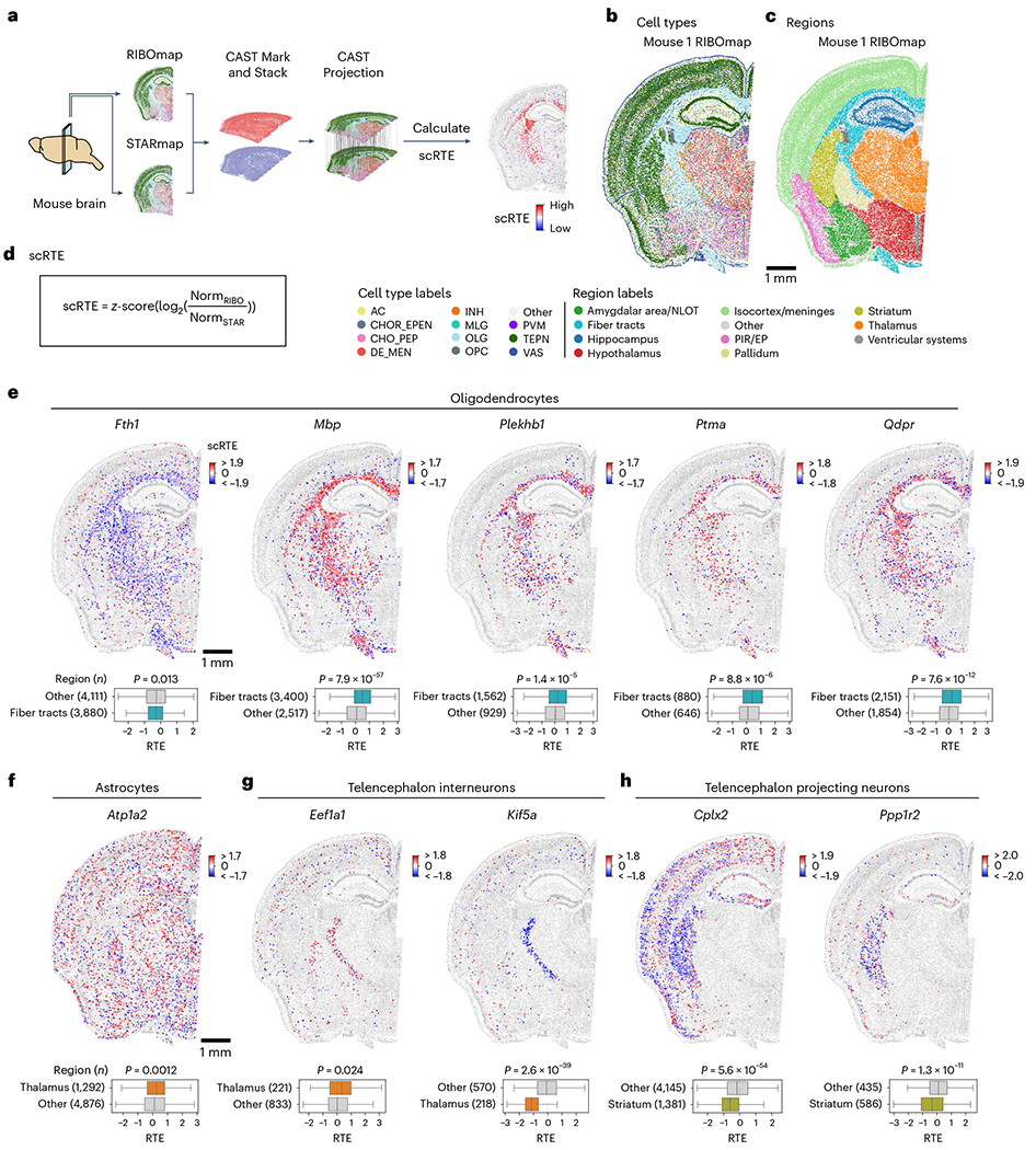
a, Schematic workflow for calculating scRTE profiles of the mouse brain. The four-sample dataset is composed of two adjacent half-brain slices taken from two different mice. Of the two adjacent slices, one was measured by RIBOmap and the other was measured by STARmap. b,c, Cell type and molecular tissue region profiles of the Mouse 1 RIBOmap sample (reference sample used in CAST Projection). AC, astrocyte; CHOR_EPEN, astro-ependymal cell; CHO_PEP, cholinergic, monoaminergic and peptidergic neuron; DE_MEN, di/mesencephalon neuron; INH, telencephalon interneuron; MLG, microglia; OLG, oligodendrocyte; PVM, perivascular macrophage; TEPN, telencephalon-projecting neuron; VAS, vascular cell. d, scRTEs were calculated using the formula. e–h, Spatially resolved and cell-type-specific scRTE profiles in Mouse 1. Cells of the annotated cell type with available scRTE values are colored by scRTE levels, other cells are colored gray. The boxplots with Kruskal–Wallis tests were used to evaluate the differences across the groups. The middle line indicates the median; the first and third quartiles are shown by the lower and upper lines, respectively; and the upper and lower whiskers extend to values not exceeding 1.5 × IQR.

After performing joint cell typing and region segmentation using CAST Mark for the four brain samples (Fig. 6b,c, Extended Data Fig. 8a–e and Methods) and CAST Stack alignment, we applied CAST Projection to project the STARmap cells to the RIBOmap cells (Fig. 6a). To validate the integration performance, we compared cell-type correspondence between query and reference cells, all of which showed accurate integration results (averaged percentage of matched labels of 85%; Extended Data Fig. 8f). After CAST Projection generated integrated tissue samples in which each cell contained both RIBOmap and STARmap measurements, we further defined single-cell relative translation efficiency (scRTE) as the normalized ratio of RIBOmap reads divided by STARmap reads in each cell (Fig. 6d and Methods).

By profiling scRTEs across all genes, we sought to analyze the spatial heterogeneity of scRTEs across cell types and tissue regions. To this end, we first grouped genes into gene modules based on their mean expression profile across different cell types, which resulted in 11 gene modules (M1–M11; Extended Data Fig. 9a,b). We then conducted cell-type-specific scRTE analysis within each cell type with gene modules that had adequate expression: M1–M5 and M9 in neurons, M6 in astrocytes, M7 in microglia, M8 in oligodendrocytes, M10 in vascular cells and M11 in astro-ependymal cells (Supplementary Table 7), which revealed widespread cell-type- and tissue-region-dependent translational regulation.

In oligodendrocytes, we detected dramatically different scRTE levels of M8 genes between fiber tracts and other regions, which involve axon ensheathment, nervous system development and myelination. For example, Mbp, Plekhb1, Ptma and Qdpr showed significantly high scRTE levels in fiber tracts, in contrast, Fth1 showed relatively low scRTE levels (Fig. 6e and Extended Data Fig. 10a). The differential translational regulation of these genes in the fiber tracts versus other regions indicates regional specialization of protein synthesis to support oligodendrocyte functions (for example myelination). In astrocytes, Atp1a2 showed higher scRTE levels in the thalamus region (Fig. 6f and Extended Data Fig. 10b). In telencephalon interneurons, the translation elongation factor Eef1a1 had higher scRTE levels in the thalamus than other regions, whereas the Kif5a exhibited lower levels in the thalamus (Fig. 6g and Extended Data Fig. 10c). In telencephalon-projecting neurons, Cplx2 and Ppp1r2 both showed lower levels in the striatum region (Fig. 6h and Extended Data Fig. 10d). These results support the heterogeneity of translation efficiency across different cell types or anatomical regions and the necessity to investigate messenger RNA translation regulation with both single-cell and spatial resolutions in future studies.

Discussion

In summary, we demonstrated that CAST enables search-and-match across samples based on their spatially resolved molecular similarities while uncovering and visualizing the variability driven by spatial differences. Such multi-technology spatial–spatial integration will benefit users to combine the strengths of different spatial technologies by cross-reference across various spatial resolutions and gene panels. Meanwhile, CAST also shows the capability for potential atlas query applications. With CAST, users could input the ROI from one tissue slice and search large reference spatial omics datasets for the best-matching tissue location for their sample.

With well-aligned samples from CAST Stack, ΔAnalysis reveals spatially heterogeneous patterns of different molecular characteristics, thereby enabling identification of disease hallmark-associated gene clusters without the need of cell-type and tissue-label annotations, which opens new perspectives toward a deeper understanding of disease, injury and regeneration mechanisms. We also integrated a spatially resolved translatome (RIBOmap) and transcriptome (STARmap) to uncover the spatial translation efficiency landscape of brain tissues at the single-cell level.

We note that the performance of CAST ΔAnalysis depends on the accuracy of tissue alignment. Thus, it is critical for the users to pay attention to the Pearson similarity scores provided in the CAST Stack results (Extended Data Fig. 3b) and filter misaligned cells and regions when needed for quality control. Meanwhile, increasing biological replicates can reduce the variations from individual samples and increase the confidence of cross-condition comparison (for example disease versus control). Furthermore, the choice of radius in the cell-centered neighborhood may influence the biological focus of ΔAnalysis (large regional changes versus local changes). Additionally, due to the warping introduced during the CAST Stack alignment, the ΔCell from ΔAnalysis may represent a relative change of local cell-type composition rather than absolute change of cell densities. If needed, the absolute cell density analysis could be performed before alignment.

CAST provides a comprehensive and modular framework for the integration and differential analyses of spatial omics data across biological replicates, measurement modalities and disease conditions with both spatial and single-cell resolutions.

Methods

Data preprocessing

In all the spatial omics datasets used, we normalized the sum of the raw read counts of each cell to $1\times {10}^4$ (referred to as norm1e4). We then applied a ${\mathrm{l}\mathrm{o}\mathrm{g}}_2$ transformation to the normalized counts (referred to as ${\mathrm{l}\mathrm{o}\mathrm{g}}_2$_norm1e4). Finally, the expression values were scaled without zero-centering (referred to as ‘scale’). Each data transformation was stored as an Anndata³⁹ layer.

CAST Mark algorithm

Given a sample with $M$ cells, the corresponding dataset is composed of each cell’s spatial coordinates $\mathrm{\Psi }\in {\mathbb{R}}^{M\times 2}$ (x and $y$ coordinates) and the feature expression matrix $\mathrm{X}\in {\mathbb{R}}^{M\times N}(N$ indicates the feature dimension, for example gene expression panel size). For each tissue sample, we first constructed the tissue graph by performing Delaunay triangulation using the spatial coordinates, resulting in an adjacency matrix $A\in {\mathbb{R}}^{M\times M}$.

The CAST Mark GNN is composed of $L$ GCNII layers¹⁶ after an optional single-layer perceptron encoder. The perceptron encoder serves as an option to reduce feature dimension and thus reduces the demand for computational resources without large compromise in performance. For each layer $l(l=\mathrm{1,2},\dots ,L-1)$,

$$H^{(l+1)}=\sigma \left(\left(\left(1-{\alpha }_l\right)\left(D^{-\frac{1}{2}}\hat{A}{D}^{-\frac{1}{2}}\right)H^{(l)}+{\alpha }_l{H}^{(0)}\right)\left(\left(1-{\beta }_l\right)I_n+{\beta }_l{W}^l\right)\right)$$

Where $\sigma (\cdot )$ is a nonlinear activation function (by default, ReLU). $\hat{A}$ is the adjacency matrix with self-loops, $D$ is its diagonal degree matrix. $H^{\left(0\right)}$ is the initial node features (for example gene expression for each cell), while $H^{\left(l\right)}$ is the feature for layer $l.{\alpha }_l$ and ${\beta }_l$ are hyperparameters for which we used their default values in the DGL package⁴⁰.

We utilized a self-supervised CCA learning objective⁴¹ to train the network, where for each sample, we first applied random node feature masks and random edge masks to the initial graph $G$ to generate two augmented views of $G:G_1=\left(\widetilde{X_1},\widetilde{A_1}\right),G_2=\left(\widetilde{X_2},\widetilde{A_2}\right)$, providing a mechanism to tolerate the intrinsic and sample-level stochasticity of gene expression and spatial locations of cells at microscopic scales. The CAST Mark $\mathrm{G}\mathrm{N}\mathrm{N}{\epsilon }_{\theta }$ is subsequently employed in parallel to create node embeddings for the two augmented views: $H_1={\epsilon }_{\theta }\left(\widetilde{X_1},\widetilde{A_1}\right)$ and $H_2={\epsilon }_{\theta }\left(\widetilde{X_2},\widetilde{A_2}\right)$. Then we normalized $\widetilde{H_1}$ and $\widetilde{H_2}$ by

$$\tilde{H}=\frac{H-\mu (H)}{\sigma (H)\sqrt{M}}$$

where $\mu$ is the mean value of each feature in the given matrix, $\sigma$ indicates the s.d. of the values in each feature and $M$ is the number of cells. The normalized ${\tilde{H}}_1$ and $\widetilde{H_2}$ are used for the CCA-based self-learning objective. The objective function is:

$$ℒ={\Vert {\tilde{H}}_1-\widetilde{H_2}\Vert }_F^2+\lambda \left({\Vert {\widetilde{H_1}}^T\widetilde{H_1}-I\Vert }_F^2+{\Vert {\widetilde{H_2}}^T\widetilde{H_2}-I\Vert }_F^2\right)$$

where the $/$ is the identity matrix and $\lambda$ is a non-negative hyperparameter.

In this study, we used $L=9$ by default. After the training process, the final graph embedding of the original graph $G$ is ${\tilde{H}}_{\text{init}}={\epsilon }_{\theta }(\tilde{X},\tilde{A})$.

Performance evaluation.

We used Pearson correlation to evaluate the similarity of the graph embeddings. We used the ARI and the percentage of consistent cells between corresponding clusters to evaluate the clustering performance.

CAST Stack algorithm

To align the spatial coordinates of samples while preserving cell organization,CAST Stack performs alignment using a gradient-descent-based rigid alignment phase followed by a nonrigid alignment phase to achieve a proper transformation.

Rigid alignment.

Affine transformation was used for rigid registration. CAST allows translation, rotation, scaling and reflection transformations, but disallows shear mappings. We set the initial coordinates of the $M$ cells in the query sample as ${\mathrm{\Psi }}^0=\left(x_i^0,y_i^0\right),i=1,\dots ,M$. For every optimization iteration $p(p=1,\dots ,P)$, the transformed coordinates were defined as ${\mathrm{\Psi }}^p=\left(x_i^p,y_i^p\right)\left(\mathrm{\Psi }=\left(x_i,y_i\right)\right.$ refers to $\left.{\mathrm{\Psi }}^p=\left(x_i^p,y_i^p\right)\right)$. The affine transformation algorithm can be written as:

$$\Psi =T_{\text{affine}}\left({\Psi }^0\right)=A{\Psi }^0+b$$

where $T_{\text{affine}}$ is the affine transformation function taking the transformation matrix $A$ and the translation vector $\mathbf{b}$ as parameters:

$$\begin{gathered} A=\left[\begin{array}{cc}\text{cos}\varphi & -\text{sin}\varphi \\ \text{sin}\varphi & \text{cos}\varphi \end{array}\right]\left[\begin{array}{ll}a\hfill & 0\hfill \\ 0\hfill & d\hfill \end{array}\right]=\left[\begin{array}{cc}a\text{cos}\varphi & -d\text{sin}\varphi \\ a\text{sin}\varphi & d\text{cos}\varphi \end{array}\right] \\ \mathbf{b}=\left[\begin{array}{l}{b}_1\hfill \\ b_2\hfill \end{array}\right] \end{gathered}$$

We reshape $A,\mathbf{b}$ into a single five-dimensional vector $\mathit{\theta }$ containing the five affine transformation parameters $a,d,\varphi ,b_1$ and $b_2$:

$$\mathit{\theta }=\left[\begin{array}{l}a\hfill \\ d\hfill \\ \varphi \hfill \\ b_1\hfill \\ b_2\hfill \end{array}\right]$$

Consequently, the affine transformation function can be formally noted as $T_{\text{affine}}\left({\mathrm{\Psi }}^0;\mathit{\theta }\right)$.

To automatically find a proper transformation, GD was performed to optimize the affine transformation parameter vector $\theta$.

The loss function J is identified as the sum of the adjusted Pearson distance $J_i$ between each query cell $i$ and its nearest reference cell:

$$J=\sum _{i=1}^M{J}_i$$

We first calculated the Pearson correlation matrix between query and reference samples using the CAST Mark graph embedding. $r_i$ is the Pearson correlation value between each query cell $i$ and its nearest reference cell. To ensure the Pearson distance has a minimum value of zero, we subtract the $r_i$ from the maximum value of the Pearson correlation matrix, thereby obtaining the adjusted Pearson distance value.

$$J_i=(\text{max}r)-r_i$$

Optimization steps are formulated as:

$$\begin{gathered} {\mathit{\theta }}_{t+1}={\mathit{\theta }}_t-\alpha {\nabla }_{\mathit{\theta }}J \\ {\nabla }_{\theta }J=\left[\begin{array}{c}\frac{\partial J}{\partial {\theta }_1}\\ \dots \\ \frac{\partial J}{\partial {\theta }_k}\\ \dots \\ \frac{\partial J}{\partial {\theta }_s}\end{array}\right] \\ \frac{\partial J}{\partial {\mathit{\theta }}_k}=\sum _{i=1}^M\frac{\partial J}{\partial {\text{Ψ}}_i}\frac{\partial {\text{Ψ}}_i}{\partial {\mathit{\theta }}_k} \end{gathered}$$

where $\alpha$ is a weighting parameter of the GD. The $\frac{\partial J}{\partial {\mathrm{\Psi }}_i}$ is the partial derivative of the J with respect to coordinate variable ${\mathrm{\Psi }}_i$:

$$\frac{\partial J}{\partial {\text{Ψ}}_i}=\left[\begin{array}{ll}\frac{\partial J}{\partial x_i}\hfill & \frac{\partial J}{\partial y_i}\hfill \end{array}\right]$$

The $\frac{\partial {\mathrm{\Psi }}_i}{\partial {\mathit{\theta }}_k}$ is the partial derivative of the coordinate variable ${\mathrm{\Psi }}_i$ with respect to ${\mathit{\theta }}_k$:

$$\begin{gathered} \frac{\partial {\text{Ψ}}_i}{\partial {\mathit{\theta }}_k}=\left[\frac{\partial x_i}{\partial {\theta }_k}\frac{\partial y_i}{\partial {\mathit{\theta }}_k}\right] \\ \frac{\partial {\text{Ψ}}_i}{\partial {\mathit{\theta }}_k}=\left[\begin{array}{cc}{x}_i\text{cos}\varphi & x_i\text{sin}\varphi \\ -y_i\text{sin}\varphi & y_i\text{cos}\varphi \\ -d{y}_i\text{cos}\varphi -a{x}_i\text{sin}\varphi & a{x}_i\text{cos}\varphi -d{y}_i\text{sin}\varphi \\ 1& 0\\ 0& 1\end{array}\right] \end{gathered}$$

Non-rigid alignment.

The FFD based on the B-spline method is used for the deformable transformation⁴². To define a spline-based FFD, we first generated a mesh grid for the spatial slice. Given the number of the control points $s$ in each dimension, the mesh spacings $g_x$ and $g_y$ are calculated by:

$$g_x=\frac{m_x}{s-1},g_y=\frac{m_y}{s-1}$$

where $m_x$ and $m_y$ represent the maximum coordinate of the slice. $\mathrm{\Omega }$ indicates $s\times s$ control points ${\omega }_{i,j}$ in the mesh grid with spacing $g_x,g_y$, respectively. All the cells (M cells) in a given query sample before B-spline alignment are identified as ${\mathrm{\Psi }}^0=\left\{\left(x_h^0,y_h^0\right)\mid \right.\left.0\le x_h^0\le m_x,0\le y_h^0\le m_y\right\},h=1,\dots ,M$. Similarly, the B-spline transformed coordinates are ${\mathrm{\Psi }}^p=\left(x_h^p,y_h^p\right)\left(\right.$ (where, $\mathrm{\Psi }=\left(x_h,y_h\right)$ indicates ${\mathrm{\Psi }}^p=\left(x_h^p,y_h^p\right)$). The B-spline transformation matrix $T_{\mathrm{B}\text{-spline}}$ for each control point is written as:

$$\text{Ψ}=T_{\text{B-spline}}\left({\text{Ψ}}^0\right)=\sum _{l=-2}^1\sum _{m=-2}^1{B}_l(u)B_m(v){\omega }_{i+l,j+m}$$

Where $i=⌊x^0/g_x⌋,j=⌊y^0/g_y⌋,u=x^0-i\times g_x,v=y^0-j\times g_y$ and where $B_l$ and $B_m$ represents the $l$-th and $m$-th basis function of the $B$-spline, respectively:

$$\begin{gathered} B_{-2}(u)=\frac{{(1-u)}^3}{6} \\ {B}_{-1}(u)=\frac{u^3}{2}-u^2+\frac{2}{3} \\ {B}_0(u)=\frac{1}{6}\left(-3u^3+3u^2+3u+1\right) \\ {B}_1(u)=\frac{u^3}{6} \end{gathered}$$

Similarly, the formula of the GD-based FFD is written as:

$$\begin{gathered} {\omega }_{t+1}={\omega }_t-\alpha {\nabla }_{\omega }J \\ {\nabla }_{\omega }J=\left[\begin{array}{ccc}\frac{\partial J}{\partial {\omega }_{0,0}}& \cdots & \frac{\partial J}{\partial {\omega }_{0,s-1}}\\ ⋮& \ddots & ⋮\\ \frac{\partial J}{\partial {\omega }_{s-1,0}}& \cdots & \frac{\partial J}{\partial {\omega }_{s-1,s-1}}\end{array}\right] \end{gathered}$$

$$\frac{\partial J}{\partial {\omega }_{i,j}}=\sum _{h=1}^M\frac{\partial J}{\partial {\text{Ψ}}_h}\frac{\partial {\text{Ψ}}_h}{\partial {\omega }_{i,j}}$$

where $\alpha$ is a weighting parameter of the GD. $\frac{\partial J}{\partial {\psi }_h}$ is the partial derivative of the $J$ with respect to coordinate variable ${\mathrm{\Psi }}_h$:

$$\frac{\partial J}{\partial {\text{Ψ}}_h}=\left[\frac{\partial J}{\partial x_h}\frac{\partial J}{\partial y_h}\right]$$

$\frac{\partial {\mathrm{\Psi }}_h}{\partial {\omega }_i}$ is the partial derivative of the coordinate variable ${\mathrm{\Psi }}_h$ with respect to ${\omega }_{i,j}$, which is equal to ${\sum }_{l=-2}^1 {\sum }_{m=-2}^1 B_l\left(u\right)B_m\left(v\right)$.

CAST Projection algorithm

We assume that a given cell will be the most similar to the cells with close distance in physical space and low-dimensional feature space. Thus, to project the features of the cells into a low-dimensional space, CAST Projection employs a sequential combination of Combat³⁰ and Harmony³¹ integration for samples with different modalities. Cosine distance is used to measure the similarity of cell features in the integrated embedding. To find the candidate cells for a given reference cell, CAST first identifies the candidate query cells within a radius of the reference cell. As different cell types exhibit varying cell distances in the space, CAST calculates the cell-type-specific cell average distance based on the Delaunay triangulation graph. By default, twice the averaged distance is utilized (in AD samples, $1.5\times$ cell distance is used, while in RIBOmap-STARmap, $3\times$ the distance is used). Among the candidate query cells, CAST identifies the cell with the closest cosine distance to project.

Simulation datasets

To generate a dataset with ground-truth cell partners across samples, we took S1 from the STARmap PLUS AD dataset as our reference and generated one simulated sample based on S1, where each cell in the synthetic sample corresponded to a ground-truth partner in the S1 sample. The simulated sample was generated by the following steps:

1. Physical location noise (nonlinear): Gaussian Process Warp⁴³ was used to perturb the spatial coordinates of the reference sample using the following parameters: noise_variance $=1\times {10}^5$; kernel_variance $=1\times {10}^5$; kernel_lengthscale $=1.0$; mean_slope $=1.0$; and mean_intercept $=0.1$.

2. Global spatial coordinates distortion (linear): the tissue sample was further changed by scaling and rotation transformations ($x$ axis, $40\mathrm{\%};y$ axis, $50\mathrm{\%}$; and rotation, ${30}^{\circ }$)

3. Gene expression noise: we applied Gaussian noise ($\mu =0,\sigma =0.2$) to the ${\mathrm{l}\mathrm{o}\mathrm{g}}_2$ norm1e4 gene expression matrix.

4. Gene feature dropout: we randomly replaced $10\mathrm{\%}$ of the values in the expression matrix using zeros.

5. Cell dropout: we randomly dropped $10\mathrm{\%}$ of cells in the simulated sample, making sure that the graph structures would be altered.

The numbers of samples per box in Fig. 2b are 79,749, 788,629, $\mathrm{1,736,756,1},\mathrm{736,756,4},\mathrm{341,890,8},\mathrm{683,780,8},\mathrm{683,780,8},\mathrm{692,641},\mathrm{8,683,780,8},\mathrm{683,780,8},\mathrm{692,641,8},\mathrm{683,780,8},\mathrm{683,780}$ and $\mathrm{8,692,641}$ for percentile groups $\mathrm{0.1,1},\mathrm{3,5},\mathrm{10,20,30,40,50,60,70,80,90}$ and 100, respectively.

Region marker gene detection

We calculated the average gene expression (${\mathrm{l}\mathrm{o}\mathrm{g}}_2$ norm1e4) in each region, which represents the gene expression abundance. Then, $z$-scores of these averaged values were calculated across all regions to quantify the degree to which expression levels vary across different regions²¹. By considering these two features and comparing them with the databases¹⁷, we identified the region marker genes (Supplementary Table 3) with help from the experts.

Querying tissue locations in spatial brain atlases using the ‘search-and-match’ strategy

We utilized the STARmap S1 sample, a subset of mouse coronal brain section that mainly contains the hippocampus region, to query against a comprehensive molecular spatial atlas of the mouse CNS²¹. The query was conducted following a two-step process. In the first step, we performed a coarse search against all candidate slices of all depths in the spatial atlas using only affine transformation to identify slices from the reference dataset with tissue location similarities. We assessed possible matching tissue locations using the CAST Stack loss values. We identified three hit slices in the reference atlas with significantly lower loss. In the second step, we performed a high-resolution alignment using the full CAST Stack (both affine and B-spline) for the query slice against the three hit slices. The reference slice with the lowest loss was determined to be the best match.

Delta-sample analysis

$\mathrm{\Delta }$Analysis was used to discover the variance driven by spatial differences across conditions. With the well-aligned samples, given one neighborhood (niche), we could get the cells and their molecular characteristics in this neighborhood with different conditions. For each cell, we defined a neighborhood as all the neighboring cells within a default $50-\mu \mathrm{m}$ radius from its center. By comparing the associated neighborhoods of aligned samples, we obtained delta statistics for molecular features such as gene expression and cell type abundance at a local resolution on the global tissue slice. After screening all cells in the sample, we obtained a global spatial gradient map of the differences in molecular features between conditions. In this study, we used these molecular features in each neighborhood:

Cell type abundance.

This means the cell counts of a certain cell type. The $\mathrm{\Delta }$Cell is the difference of the cell type abundance in each comparison. For example, for one of the combinations (S8–S3) in the 13-month comparison, $\mathrm{\Delta }{\mathrm{Cell}}_i\left(\text{Oligo}\right)={\text{Cell}}_{c_1}\left(\text{Oligo}\right)-{\text{Cell}}_{c_2}\left(\text{Oligo}\right)$, where ${\text{Cell}}_{c_1}\left(\text{Oligo}\right)$ is the abundance of the oligodendrocytes in the disease sample S8, while ${\text{Cell}}_{c_2}\left(\text{Oligo}\right)$ is the abundance of the oligodendrocytes in the control sample S3. The strategy was applied for gene expression, CCAs and CCIs.

Gene expression.

$\mathrm{\Delta }$Exp is the difference of the average gene expresion (log₂_norm1e4) in each comparison. The spatial amyloid plaque-induced genes (PIGs) are identified by the following criteria: (1) $\mathrm{\Delta }\mathrm{E}\mathrm{x}\mathrm{p}>0.1$; (2) the spatial correlation (Pearson $r$) between the $\mathrm{\Delta }\mathrm{E}\mathrm{x}\mathrm{p}$ and plaque score is greater than 0.1; and (3) the false discovery rate values of the Wilcoxon rank sum test for the differential expression analysis is $<0.1$.

Cell–cell adjacencies.

$△CCA$ is defined as the difference of the CCA value of the given cell type pairs. The CCA value between cell type $A$ and B is defined as the number of A–B edges within a two-hop neighborhood on the Delaunay tissue graph.

Cell–cell interactions.

$\mathrm{\Delta }\mathrm{C}\mathrm{C}\mathrm{I}$ is defined as the difference of the CCI degree of a ligand–receptor pair in each comparison derived as in CellPhoneDB⁴⁴. The CCI degree is calculated by Squidpy (v.1.2.2)⁴⁵ with the normalized counts (norm1e4).

Plaque score.

This is the sum of the plaque area in each niche. We filtered plaques with the area less than 300 pixels ($~30\mu {\mathrm{m}}^2$) in the image.

Tau score (value).

This is the sum of the tau rate in the cells. The tau rate is defined as the ratio between the tau area and the cell area in each cell.

To interrogate the spatially resolved molecular differences among different age groups, we used two comparisons: 8-month disease and control (8 months), 13-month disease and control (13 months; Fig. 4a).

Hot-zone visualization.

The contour map visualization was adopted to visualize the spatial gradients of $\mathrm{\Delta }$Analysis features and highlight the loci with locally enriched differences across conditions in an unsupervised, label-free way. For a given $\mathrm{\Delta }$Analysis feature, radial basis function interpolation was used to generate the contour lines (Rbf function in the SciPy package and contour function in the matplotlib package). The hot-zones were defined as the loci surrounded by the contours (by default, the top 20% percentile contour).

scRTE analysis

To measure the translation efficiency among cells regardless of the different expression distributions due to the different technologies or samples, we introduced the scRTE metric for each cell as the following formula (scTE represents single cell translation efficiency):

$$\begin{gathered} {\text{scTE}}_{i,j}={\text{log}}_2\left(\frac{{\text{RIBO}}_{i,j}}{\text{STAR}{R}_{i,j}}\right) \\ {\mathit{scRTE}}_{i,j}=\frac{{\mathit{scTE}}_{i,j}-{\mu }_i}{{\sigma }_i} \end{gathered}$$

where ${\mathrm{R}\mathrm{I}\mathrm{B}\mathrm{O}}_{ij}$ and ${\mathrm{S}\mathrm{T}\mathrm{A}\mathrm{R}}_{i,j}$ are the RIBOmap and STARmap normalized counts (norm1e4) of the gene $i$ in cell $j$. The ${\mu }_i$ and ${\sigma }_i$ are the average value and s.d. of the ${\mathrm{s}\mathrm{c}\mathrm{T}\mathrm{E}}_{ij}$ of the gene $i$ across all cells. The $\mathrm{s}\mathrm{c}\mathrm{R}\mathrm{T}\mathrm{E}{E}_{i,j}$ is the $z$-score of the ${\mathrm{s}\mathrm{c}\mathrm{T}\mathrm{E}}_{i,j}$ over all cells.

Once we calculate the scRTE values of each cell in a given gene, scRTE levels at different locations may not be consistent. To detect the spatial variability of the scRTE levels in each gene, we used the s.d. of the scRTE values of each gene to measure the degree of heterogeneity for each gene. Meanwhile, the Kruskal–Wallis test was used to evaluate whether the scRTE levels are significantly different between the cell types or regions. As the STARmap sample in Mouse 2 is truncated at the hypothalamus, cortical subplate and olfactory cortical regions, our analysis focuses solely on the overlapping region within the Mouse 2 sample.

Although scRTE is not the absolute ratio of ribosome-bound RNA versus the total RNA as RIBOmap and STARmap were measured from two different samples using different technologies, it reflects the rank of relative translational levels compared to other cells in the dataset. We reason that scRTE is a more robust metric across samples while reflecting spatial heterogeneity of translation efficiency.

Region segmentation of mouse half-brain datasets

We first performed CAST Mark training on the normalized expression (norm1e4) with Combat batch correction³⁰ of 1,082 highly variable genes across all four half-brain samples. We then performed $k$-means ($k=20$) clustering on the CAST Mark graph embedding. Among the 20 clusters, we selected the most under-segmented cluster (region 3) and further subclustered region 3 into 10 subclusters, yielding a total of 29 clusters. We then visually examined all 29 regions. Using the Allen Brain Atlas^17,18 as the reference, we merged over-segmented regions consistent with established brain anatomy. We also separated physically segregated areas belonging to the same $k$-means cluster into two regions (HY, hypothalamus and LH, lateral habenula). Consequently, we confirmed a total of 23 brain subregions. Finally, we concluded these 23 brain subregions into 10 top-level brain regions based on the Allen Brain Atlas.

Gene clustering

The gene expression (${\mathrm{l}\mathrm{o}\mathrm{g}}_2$_norm1e4) of the four samples were first averaged across the cell types within each sample, respectively. Subsequently, the average expression values were standardized by calculating the $z$-score within each sample. Eight hundred eighty-four highly abundant genes with sufficient expression and scRTE values in each sample were used in this analysis. The standardized vectors for RIBOmap and STARmap were jointly clustered with the Louvain algorithms from Seurat (v.4.0.3). We then used ComplexHeatmap (v.2.10.0) to visualize the clusters. For the gene clustering based spatial pattern ($\mathrm{\Delta }$Exp spatial pattern), the Pearson correlation matrix between the genes was first calculated. Then the matrix was used for Leiden clustering (Scanpy⁴⁶, v.1.9.1).

Enrichment analysis

To identify the enriched GO and KEGG pathway terms, gprofiler2 (v.0.2.1) was applied for the enrichment analysis. The enriched terms were further visualized by the EnrichmentMap plugin in Cytoscape (v.3.9.1). For visualization, clusters containing fewer than five nodes were excluded. For the spatially resolved PIGs, the GO and KEGG pathway enrichment analyses were conducted with clusterProfiler (v.3.18.1)⁴⁷.

Benchmark with PASTE alignment

We used the pairwise_align (GPU mode) and center_align (CPU mode; not available in GPU mode) in PASTE to run the alignment tasks of different samples with default parameters. The NVIDIA RTX A5000 (24 GB VRAM) GPU was used in the task. We only presented the available results for the eight AD sample and Visium datasets (Supplementary Fig. 6), as PASTE was unable to execute the half-brain alignment tasks due to memory limitations (limited to CPU 80 GB RAM).

For the Visium dataset, we set min_counts $=15$ in the function sc.pp.filter_genes and min_counts $={100}^{-}$ in the function sc.pp.filter_cells to filter the low-expressed genes and voxels. The reference slice was Visium1 (Mouse Brain Coronal Section 1) and the query slice was Visium2 (Mouse Brain Coronal Section 2). Raw expression data was used. Default values of parameter numItermax and $\alpha$ were used for the function pairwise_align.

For the eight AD sample dataset, we set min_counts = 200 in the function sc.pp.filter_cells to filter the low-expressed genes. The raw expression data was used. Default values of parameters were used for the function pairwise_align and center_align. In pairwise alignment tasks, S1 was used as the reference slice and other slices were used as the query slices.

Reporting summary

Further information on research design is available in the Nature Portfolio Reporting Summary linked to this article.

Data availability

The RIBOmap and STARmap datasets are available from (RIBOmap_mouse1, STARmap_mouse1 and RIBOmap_mouse2) https://singlecell.broadinstitute.org/single_cell/study/SCP1835 and (STARmap_mouse2) https://singlecell.broadinstitute.org/single_cell/study/SCP2203). The AD STARmap PLUS datasets (S1–S8, S64_1 and S64_2) are publicly available at https://singlecell.broadinstitute.org/single_cell/study/SCP1375/. The mouse brain atlas dataset used is available at https://singlecell.broadinstitute.org/single_cell/study/SCP1830. The two Visium datasets (Mouse Brain Coronal Section 1 (FFPE) and Mouse Brain Coronal Section 2 (FFPE)) are available from https://www.10xgenomics.com/resources/datasets/mouse-brain-coronal-section-1-ffpe-2-standard and https://www.10xgenomics.com/resources/datasets/mouse-brain-coronal-section-2-ffpe-2-standard. The MERFISH dataset (co1_slice37 in co1_sample13) is available from https://doi.brainimagelibrary.org/doi/10.35077/act-bag. The Slide-seq dataset (slice042) is available from https://docs.braincelldata.org/downloads/index.html. The two Stereo-seq MOSTA datasets (E16.5_E2S5 and E16.5_E2S6) are available from https://db.cngb.org/stomics/mosta/download/.

Code availability

The code and demos of CAST have been deposited to GitHub at (https://github.com/wanglab-broad/CAST) and Zenodo (https://zenodo.org/doi/10.5281/zenodo.12215314 (ref. 48)). The implementation of CAST, as well as the tutorials, are available in the demo pipeline files and CAST document page (https://cast-tutorial.readthedocs.io/en/latest/).

Extended Data

Extended Data Fig. 1 |. CAST Mark identifies the common spatial features between the simulated and real samples.

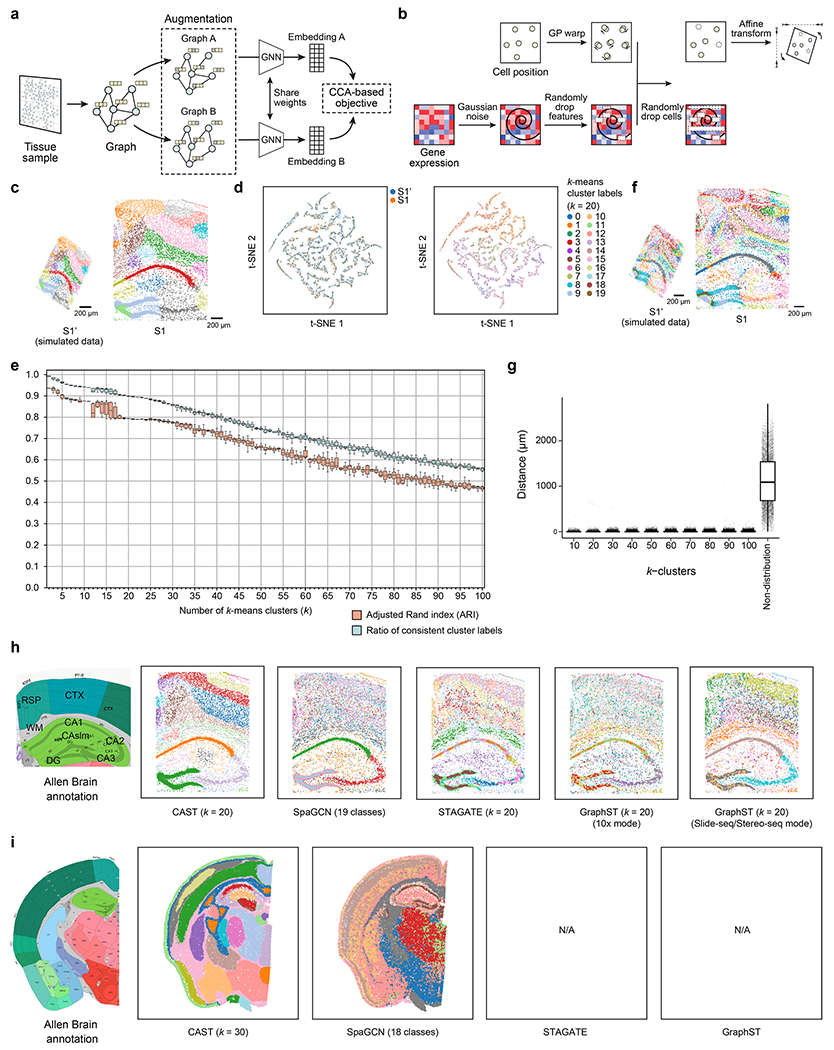
a, The schematic workflow of the self-supervised learning framework used in CAST Mark. b, The simulation strategy to generate the simulated dataset S1’ from the real sample S1 (8 month, control) in STARmap PLUS dataset (Methods). c, The k-means (k = 20) clustering results of the graph embedding generated by CAST Mark. Different colors in the cells indicate different clusters of the graph embedding. d, The t-SNE visualization of the spatial embedding labeled with samples (left) and k-means clusters (k = 20, right). e, The clustering performance adjusted Rand index (ARI) and the percentage of the consistent cells in different numbers of the clusters (k). Each box contains 10 technical replicates using different random seeds. f, The k-means (k = 100) clustering results of the spatial embedding generated by CAST Mark. g, The distance distribution of the cells in different k-clusters and non-distribution groups (sample size = 8,789 for each group). The distance indicates each cell in the simulated sample S1’ to the closest one with the same cluster in the S1 sample. In the boxplots of e and g, the middle line indicates the median; the first and third quartiles are shown by the lower and upper lines, respectively; the upper and lower whiskers extend to values not exceeding 1.5 times the IQR. h, Enabled by a deep GNN and a self-supervised CCA objective, CAST Mark outperforms existing GNN-based methods (SpaGCN, STAGATE, GraphST) in tissue segmentation tasks at a ~ 9,800-cell scale. Segmentation results were colored by clusters, shown along with brain annotation from the Allen Institute^17,18. i, Tissue segmentation was performed on a STARmap dataset collected on a single coronal slice of mouse half brain⁷. The performance of CAST Mark scales up to the ~60,000-cell scale (a typical coronal slice of mouse half brain), outperforming SpaGCN¹¹, while GraphST and STAGATE fail to handle this large dataset (5,413 genes) at single-cell resolution.

Extended Data Fig. 2 |. CAST Mark identifies consistent regions across age, strain, and disease conditions.

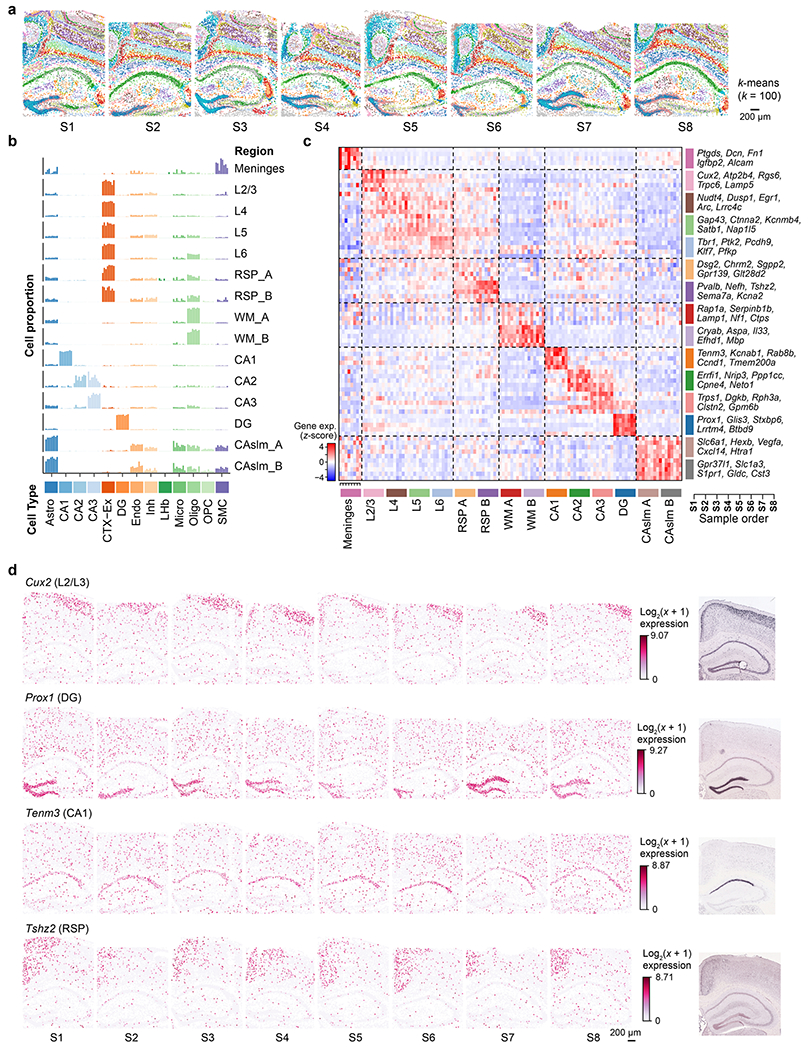
a, The k-means (k = 100) clustering result of graph embeddings generated by CAST Mark in the samples S1–S8. Different colors in the cells indicate the different clusters of the embedding. b, The bar plots show the consistent cell proportions of each cell type in each sample (Ordered from S1 to S8) and region. Astro, astrocyte; CA1, CA1 excitatory neuron; CA2, CA2 excitatory neuron; CA3, CA3 excitatory neuron; CTX-Ex, cortex excitatory neuron; DG, dentate gyrus; Endo, endothelial cell; Inh, inhibitory neuron; Micro, microglia; Oligo, oligodendrocyte; OPC, oligodendrocyte precursor cell; SMC, smooth muscle cell. c, The z-score of the mean value of the log₂_norm1e4 (Methods) profiles of region marker genes (Supplementary Table 3) in each region (Ordered from S1 to S8) shows that CAST Mark identifies consistent regions across multiple samples. d, The gene expression of region markers Cux2 (L2/L3), Prox1 (DG), Tenm3 (CA1) and Tshz2 (RSP) across 8 samples (Ordered from S1 to S8). The region marker genes are validated by the ISH images from the Allen Brain Atlas¹⁷.

Extended Data Fig. 3 |. Pearson correlation of CAST Mark graph embedding between cells is a robust similarity metric for cell locations across samples.

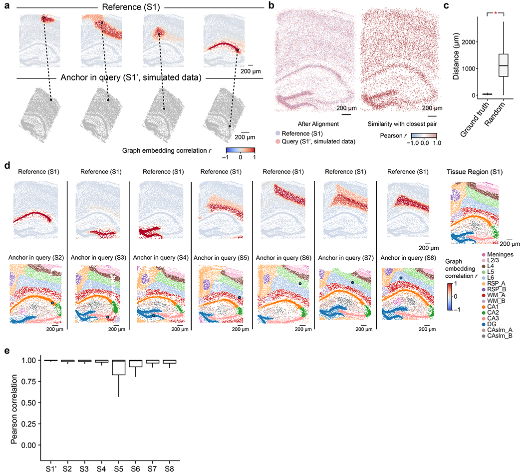
a, Given the query cell in the query slice (simulated dataset S1’), the cells in the reference sample (S1) are colored by Pearson’s correlation of the graph embedding between the reference cell and the given query cell in the query sample (S1’). b, Left panel, the coordinates of the S1 and the S1’ after alignment (same as Fig. 2d). Right panel, each cell in the query sample is colored by Pearson correlation of the graph embedding between itself and its closest pair in the reference sample. c, The boxplots show the significantly closer physical distances (One-way ANOVA; p-value < 2.2e-16) of the correct cell pair (ground truth, mean = 37.82 μm, sample size = 8,789) than the ones in random cell pairs (Random, mean = 1133.49 μm, sample size = 8,789). d, Given a query cell in the query sample (S2–S8), the cells in the reference sample (S1) are colored by Pearson’s correlation of the graph embedding between the reference cells and the given query cell. Cells with high Pearson’s correlation in the reference sample show similar relative spatial locations to the query cell. In the bottom panel, cells in the query samples are colored by tissue region labels produced by CAST Mark (same as Fig. 1c for visualization). e, The boxplots show the high Pearson correlation of the graph embedding between the cells in query samples (S1’ and S2–S8) and the reference cell with the closest physical distance in the reference sample (S1). Average Pearson r: 0.99 (S1’, n = 8,789), 0.95 (S2, n = 8,506), 0.94 (S3, n = 9,428), 0.93 (S4, n = 8,034), 0.82 (S5, n = 8,202), 0.88 (S6, n = 8,186), 0.91 (S7, n = 9,634) and 0.92 (S8, n = 10,372). In the boxplots in c and e, the middle line indicates the median; the first and third quartiles are shown by the lower and upper lines, respectively; the upper and lower whiskers extend to values not exceeding 1.5 times the IQR.

Extended Data Fig. 4 |. CAST has wide utility across various spatial technologies.

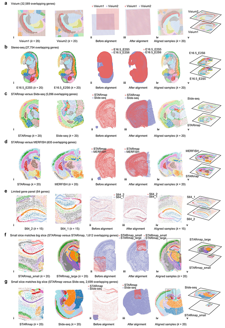
a-g, CAST automatically searches and matches shared tissue anatomy in different technologies at high spatial resolution: a, Visium (Visium1: Mouse Brain Coronal Section 1; Visium2: Mouse Brain Coronal Section 2); b, Stereo-seq⁴; c, STARmap (STARmap_mouse1⁷) versus Slide-seq²⁰; d, STARmap (STARmap_mouse1) versus MERFISH¹⁹; e, Two STARmap samples with limited gene panels⁵ (both have 64 genes); f, STARmap versus STARmap. STARmap_small is S1 and STARmap_large is STARmap_mouse1; g, STARmap (S1) versus Slide-seq. i, joint k-means clustering results of CAST Mark graph embeddings of two samples, colored by joint clusters. ii,iii, spatial coordinates of the query sample (colored pink) and the reference sample (colored blue) before (ii) and after (iii) alignment. iv,v, aligned samples colored by joint k-means clustering results of the graph embeddings (iv panel, 2D visualization; v panel, 3D visualization).

Extended Data Fig. 5 |. ΔAnalysis identifies the spatial changes of molecular characteristics between disease and normal conditions.

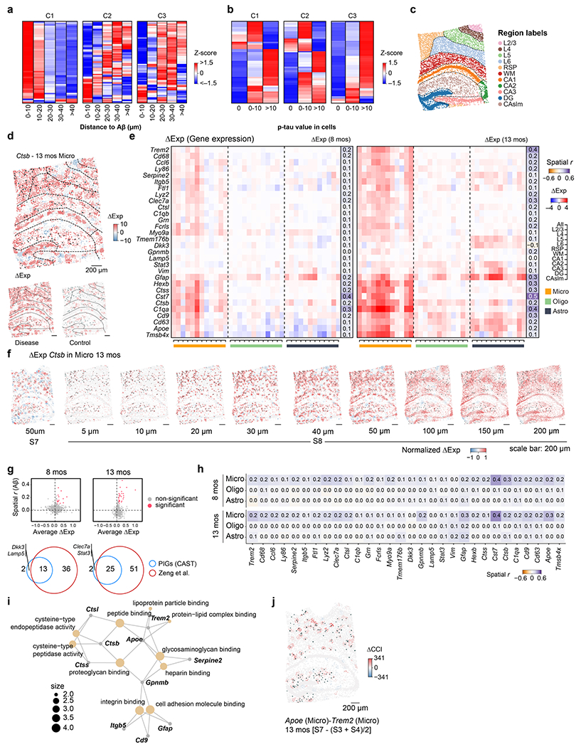
a,b, The ΔExp profiles of genes within each cluster in different cell groups. The cells are grouped by their distances to the nearest Aβ plaque (a) and by their tau values (b). c, The niche centers (cell) colored by the different regions. d, The spatial gradient map (S8 coordinates) shows the ΔExp of the Ctsb gene in microglia and 13 mos comparison (S8 − (S3 + S4) / 2). The disease sample shows the Ctsb gene expression in microglia cells of S8, while the control one shows the average values of S3 and S4. The size of dark green dots indicates the Aβ plaque area. The dash lines indicate different CAST Mark regions (c). e, The average delta gene expression (ΔExp) of the plaque-induced genes in different regions, cell types and comparisons. The average spatial correlation (Pearson r) between the overall (gene expression in all cells) ΔExp and the Aβ-plaque score are listed aside. The values of 4 combinations in each comparison are averaged (13 mos comparison: S7 – S3, S7 – S4, S8 – S3, S8 – S4; 8 mos comparison: S5 – S1, S5 – S2, S6 – S1, S6 – S2). f, The ΔExp of the Ctsb gene in microglia and 13 mos comparison (S7 − (S3 + S4) / 2, R = 50 μm; S8 − (S3 + S4) / 2, R from 5 μm to 200 μm). For visualization, the ΔExp pattern in d (top) is also displayed here. g, The scatter plots show the overall ΔExp of each gene and its spatial correlation with Aβ plaque score in different comparisons. Venn diagrams show the overlap of the identified plaque-induced genes with the ones identified in initial study. h, The average spatial correlation (Pearson r) between the ΔExp of each plaque-induced gene and the Aβ-plaque score. Similar to e, the values of 4 combinations in each comparison are averaged. i, The GO enrichment analysis of the plaque-induced genes. j, Analogous to d, the ΔCCI pattern of the Apoe (Micro) - Trem2 (Micro) in 13 mos comparison (S7 − (S3 + S4) / 2).

Extended Data Fig. 6 |. Alignment and ΔAnalysis results between injured and normal brain hemispheres during axolotl tissue regeneration.

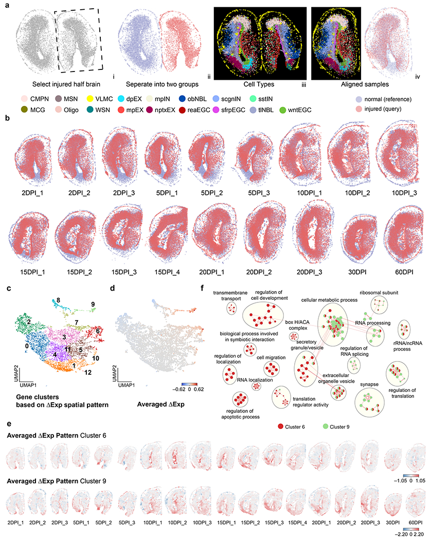
a, An example of injured versus normal brain hemispheres before and after alignment. i,ii, CAST was applied to separate injured and healthy hemispheres. iii, cell-type profiles of the sample reported by Wei et al.²⁹ iv, visualization of aligned injured and intact hemispheres. b, Alignment results across different DPI stages. The aligned result of sample 2DPI_2 is also used in a. c, UMAP clustering results of the ΔExp spatial patterns across all aligned slices. d, UMAP of the averaged ΔExp of each gene across all samples. e, The averaged ΔExp profiles (log₂_norm1e4) of Clusters 6 and 9 across all stages. f, Comparative GO analysis of the genes in Clusters 6 and 9.

Extended Data Fig. 7 |. CAST Projection accurately preserves gene expression and spatial relationships in cells across samples.

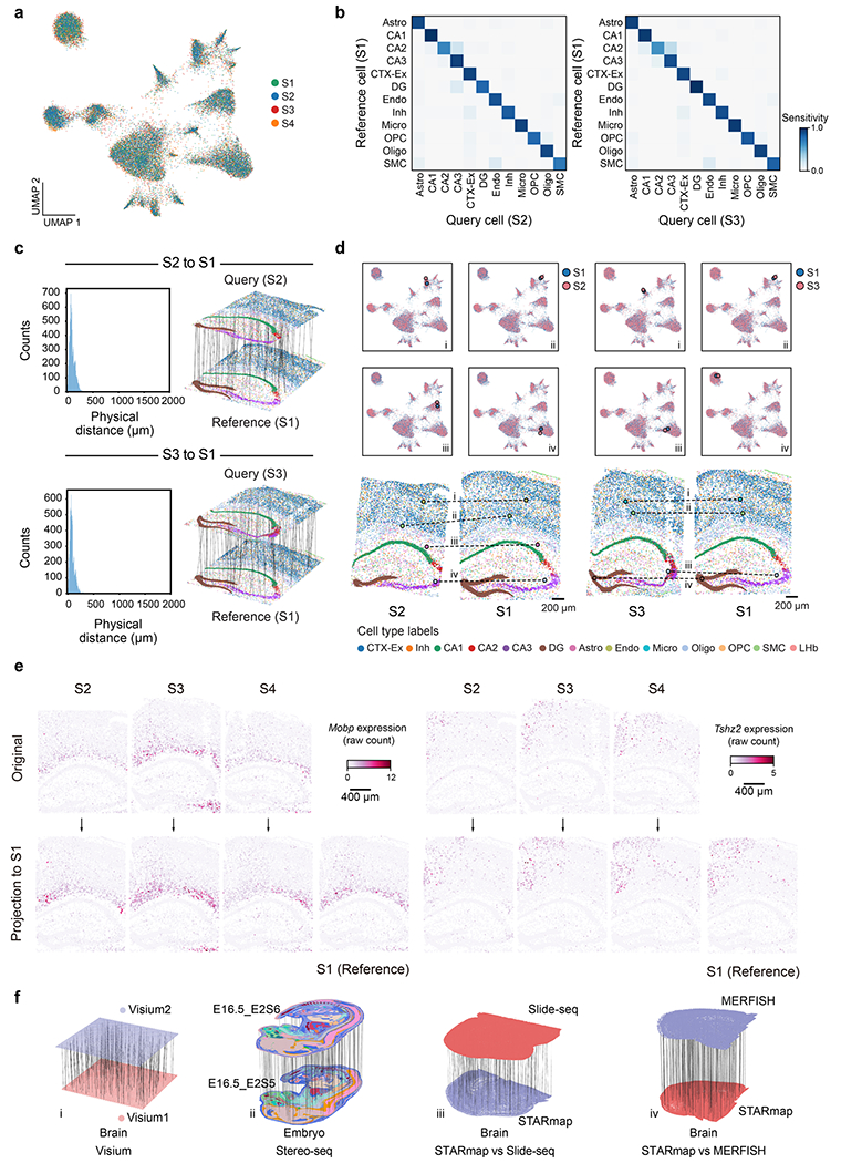
a, UMAP of Combat³⁰ and Harmony³¹ integrated embedding across S1–S4 samples (control samples) shows that the 4 samples are well integrated in different clusters. Different colors represent different samples. b, Confusion matrix of the projection performance (S2 to S1, True positive rate (TP) = 0.88; S3 to S1, TP = 0.91). The cell types with more than 10 cells in the reference sample are visualized. c, Left panel: The distribution of the physical distance in the spatial single-cell projection of the S2 to S1 (top) and S3 to S1 (bottom). Right panel: Schematic for CAST Projection results. Dashed lines (100 randomly sampled alignment pairs for visualization) connect cells from the query sample (top panel: S2, bottom panel: S3) with its destination cell in the reference sample (S1). d, CAST Projection assignment examples between S2 to S1 (left panel) and S3 to S1 (right panel) in the UMAP plots (top, S2 and S3, light red; S1, blue) and real samples (bottom, the colors of the cells are colored by cell types). e, Mobp and Tshz2 gene expression (raw count) profile in the original samples (top, S2–S4) and projected samples (bottom). f, CAST Projection is applicable across major spatial technologies and organs. i, Visium (Visium1: Mouse Brain Coronal Section 1; Visium2: Mouse Brain Coronal Section 2); ii, Stereo-seq; iii, STARmap (STARmap_mouse1) versus Slide-seq; iv, STARmap (STARmap_mouse1) versus MERFISH. CAST Projection preserves original single-cell resolution on mouse half brain and whole mouse embryo samples. Dashed lines (200 randomly sampled assignment pairs for visualization) connect cells from the query sample with its destination cell in the reference sample. In ii, the cells are colored by cell labels in the initial study.

Extended Data Fig. 8 |. Integration of spatially resolved single-cell ribosome profiling and gene expression profiling.

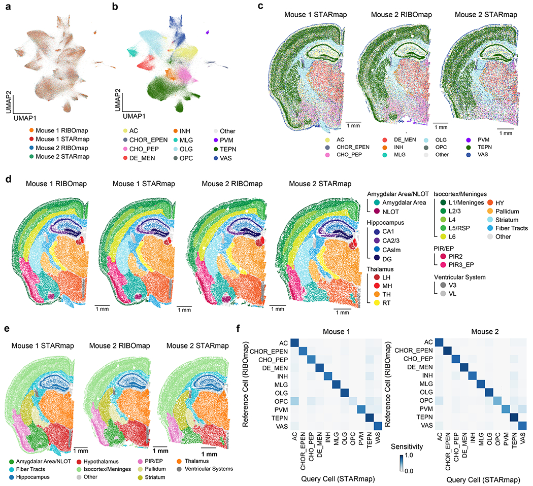
a,b, UMAP visualization of the Integrated RIBOmap and STARmap datasets. Each cell is colored by datasets (a) or cell type (b). c, Cell type profiles of Mouse 1 STARmap, Mouse 2 RIBOmap and Mouse 2 STARmap samples. d,e, Tissue region (e) and sub-region (d) profiles of samples generated using CAST Mark. The hierarchy of tissue regions are shown in the legends (right panel, d). HY, hypothalamus; LH, lateral habenula; MH, medial habenula; NLOT, nucleus of the lateral olfactory tract; PIR2, piriform area, pyramidal layer; PIR3_EP, piriform area, polymorph layer and endopiriform nucleus; RT, reticular nucleus of the thalamus; TH, thalamus; V3, third ventricle; VL, lateral ventricle. f, Confusion matrix of the projection results (Mouse 1, True positive rate (TP) = 0.84; Mouse 2, TP = 0.86).

Extended Data Fig. 9 |. Gene modules identified by co-clustering of RIBOmap and STARmap data in four samples.

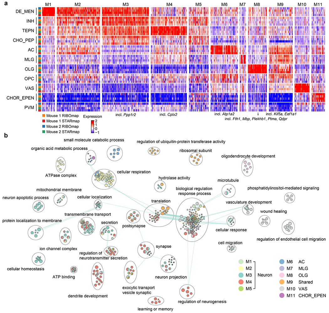
a, Genes are clustered into 11 distinct clusters by co-clustering of RIBOmap and STARmap data in four samples (z-score expression). Example genes shown in Fig. 6e–h are marked below the gene modules they belong to. b, Enriched GO terms in each gene module are grouped by terms and colored by gene modules. In the enrichment map, nodes represent the enriched GO terms, while the size of the node corresponds to the number of genes in the GO terms. The edges between nodes indicate the overlapping genes between the GO terms.

Extended Data Fig. 10 |. Examples of the cell-type specific scRTE patterns across different genes.

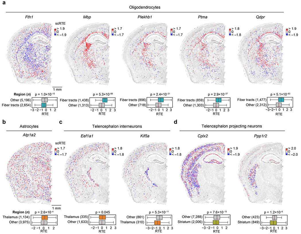
a-d, Spatially resolved and cell type specific scRTE profiles in Mouse 2. Cells of the annotated cell type (above) and with available scRTE values are colored by scRTE levels, other cells are colored gray. The boxplots with Kruskal-Wallis tests are used to evaluate the differences across the groups. The middle line indicates the median; the first and third quartiles are shown by the lower and upper lines, respectively; the upper and lower whiskers extend to values not exceeding 1.5 times the IQR.

References

- 1.Shah S, Lubeck E, Zhou W & Cai L In situ transcription profiling of single cells reveals spatial organization of cells in the mouse hippocampus. Neuron 92, 342–357 (2016). [DOI] [PMC free article] [PubMed] [Google Scholar]
- 2.Moffitt JR et al. Molecular, spatial, and functional single-cell profiling of the hypothalamic preoptic region. Science 362, eaau5324 (2018). [DOI] [PMC free article] [PubMed] [Google Scholar]
- 3.Stickels RR et al. Highly sensitive spatial transcriptomics at near-cellular resolution with Slide-seqV2. Nat. Biotechnol 39, 313–319 (2021). [DOI] [PMC free article] [PubMed] [Google Scholar]
- 4.Chen A. et al. Spatiotemporal transcriptomic atlas of mouse organogenesis using DNA nanoball-patterned arrays. Cell 185, 1777–1792.e21 (2022). [DOI] [PubMed] [Google Scholar]
- 5.Zeng H. et al. Integrative in situ mapping of single-cell transcriptional states and tissue histopathology in a mouse model of Alzheimer’s disease. Nat. Neurosci 26, 430–446 (2023). [DOI] [PMC free article] [PubMed] [Google Scholar]
- 6.Lu T, Ang CE & Zhuang X Spatially resolved epigenomic profiling of single cells in complex tissues. Cell 185, 4448–4464.e17 (2022). [DOI] [PMC free article] [PubMed] [Google Scholar]
- 7.Zeng H. et al. Spatially resolved single-cell translatomics at molecular resolution. Science 380, eadd3067 (2023). [DOI] [PMC free article] [PubMed] [Google Scholar]
- 8.Goltsev Y. et al. Deep profiling of mouse splenic architecture with CODEX multiplexed imaging. Cell 174, 968–981.e15 (2018). [DOI] [PMC free article] [PubMed] [Google Scholar]
- 9.Zeira R, Land M, Strzalkowski A & Raphael BJ Alignment and integration of spatial transcriptomics data. Nat. Methods 19, 567–575 (2022). [DOI] [PMC free article] [PubMed] [Google Scholar]
- 10.Yuan Y & Bar-Joseph Z GCNG: graph convolutional networks for inferring gene interaction from spatial transcriptomics data. Genome Biol. 21, 300 (2020). [DOI] [PMC free article] [PubMed] [Google Scholar]
- 11.Hu J. et al. SpaGCN: Integrating gene expression, spatial location and histology to identify spatial domains and spatially variable genes by graph convolutional network. Nat. Methods 18, 1342–1351 (2021). [DOI] [PubMed] [Google Scholar]
- 12.Dong K & Zhang S Deciphering spatial domains from spatially resolved transcriptomics with an adaptive graph attention auto-encoder. Nat. Commun 13, 1739 (2022). [DOI] [PMC free article] [PubMed] [Google Scholar]
- 13.Fischer DS, Schaar AC & Theis FJ Modeling intercellular communication in tissues using spatial graphs of cells. Nat. Biotechnol 41, 332–336 (2023). [DOI] [PMC free article] [PubMed] [Google Scholar]
- 14.Palla G, Fischer DS, Regev A & Theis FJ Spatial components of molecular tissue biology. Nat. Biotechnol 40, 308–318 (2022). [DOI] [PubMed] [Google Scholar]
- 15.Long Y. et al. Spatially informed clustering, integration, and deconvolution of spatial transcriptomics with GraphST. Nat. Commun 14, 1155 (2023). [DOI] [PMC free article] [PubMed] [Google Scholar]
- 16.Chen M, Wei Z, Huang Z, Ding B & Li Y Simple and deep graph convolutional networks. in Proceedings of the 37th International Conference on Machine Learning 1725–1735 (PMLR, 2020). [Google Scholar]
- 17.Lein ES et al. Genome-wide atlas of gene expression in the adult mouse brain. Nature 445, 168–176 (2007). [DOI] [PubMed] [Google Scholar]
- 18.Wang Q. et al. The Allen Mouse Brain Common Coordinate Framework: a 3D reference atlas. Cell 181, 936–953.e20 (2020). [DOI] [PMC free article] [PubMed] [Google Scholar]
- 19.Zhang M. et al. Molecularly defined and spatially resolved cell atlas of the whole mouse brain. Nature 624, 343–354 (2023). [DOI] [PMC free article] [PubMed] [Google Scholar]
- 20.Langlieb J. et al. The molecular cytoarchitecture of the adult mouse brain. Nature 624, 333–342 (2023). [DOI] [PMC free article] [PubMed] [Google Scholar]
- 21.Shi H. et al. Spatial atlas of the mouse central nervous system at molecular resolution. Nature 622, 552–561 (2023). [DOI] [PMC free article] [PubMed] [Google Scholar]
- 22.Rood JE et al. Toward a common coordinate framework for the human body. Cell 179, 1455–1467 (2019). [DOI] [PMC free article] [PubMed] [Google Scholar]
- 23.Armingol E, Officer A, Harismendy O & Lewis NE Deciphering cell–cell interactions and communication from gene expression. Nat. Rev. Genet 22, 71–88 (2021). [DOI] [PMC free article] [PubMed] [Google Scholar]
- 24.Yeh FL, Wang Y, Tom I, Gonzalez LC & Sheng M TREM2 binds to apolipoproteins, including APOE and CLU/APOJ, and thereby facilitates uptake of amyloid-β by microglia. Neuron 91, 328–340 (2016). [DOI] [PubMed] [Google Scholar]
- 25.Krasemann S. et al. The TREM2–APOE pathway drives the transcriptional phenotype of dysfunctional microglia in neurodegenerative diseases. Immunity 47, 566–581.e9 (2017). [DOI] [PMC free article] [PubMed] [Google Scholar]
- 26.Parhizkar S. et al. Loss of TREM2 function increases amyloid seeding but reduces plaque-associated ApoE. Nat. Neurosci 22, 191–204 (2019). [DOI] [PMC free article] [PubMed] [Google Scholar]
- 27.Wolfe CM, Fitz NF, Nam KN, Lefterov I & Koldamova R The role of APOE and TREM2 in Alzheimer’s disease-current understanding and perspectives. Int. J. Mol. Sci 20, 81 (2019). [DOI] [PMC free article] [PubMed] [Google Scholar]
- 28.Nandrot EF et al. Essential role for MFG-E8 as ligand for αvβ5 integrin in diurnal retinal phagocytosis. Proc. Natl Acad. Sci. USA 104, 12005–12010 (2007). [DOI] [PMC free article] [PubMed] [Google Scholar]
- 29.Wei X. et al. Single-cell Stereo-seq reveals induced progenitor cells involved in axolotl brain regeneration. Science 377, eabp9444 (2022). [DOI] [PubMed] [Google Scholar]
- 30.Johnson WE, Li C & Rabinovic A Adjusting batch effects in microarray expression data using empirical Bayes methods. Biostatistics 8, 118–127 (2007). [DOI] [PubMed] [Google Scholar]
- 31.Korsunsky I. et al. Fast, sensitive and accurate integration of single-cell data with Harmony. Nat. Methods 16, 1289–1296 (2019). [DOI] [PMC free article] [PubMed] [Google Scholar]
- 32.Spitzer MH et al. An interactive reference framework for modeling a dynamic immune system. Science 349, 1259425 (2015). [DOI] [PMC free article] [PubMed] [Google Scholar]
- 33.Baron M. et al. A single-cell transcriptomic map of the human and mouse pancreas reveals inter- and intra-cell population structure. Cell Syst. 3, 346–360.e4 (2016). [DOI] [PMC free article] [PubMed] [Google Scholar]
- 34.Haghverdi L, Lun ATL, Morgan MD & Marioni JC Batch effects in single-cell RNA-sequencing data are corrected by matching mutual nearest neighbors. Nat. Biotechnol 36, 421–427 (2018). [DOI] [PMC free article] [PubMed] [Google Scholar]
- 35.Biancalani T. et al. Deep learning and alignment of spatially resolved single-cell transcriptomes with Tangram. Nat. Methods 18, 1352–1362 (2021). [DOI] [PMC free article] [PubMed] [Google Scholar]
- 36.Kleshchevnikov V. et al. Cell2location maps fine-grained cell types in spatial transcriptomics. Nat. Biotechnol 40, 661–671 (2022). [DOI] [PubMed] [Google Scholar]
- 37.Stuart T. et al. Comprehensive integration of single-cell data. Cell 177, 1888–1902.e21 (2019). [DOI] [PMC free article] [PubMed] [Google Scholar]
- 38.Welch JD et al. Single-cell multi-omic integration compares and contrasts features of brain cell identity. Cell 177, 1873–1887.e17 (2019). [DOI] [PMC free article] [PubMed] [Google Scholar]
- 39.Virshup I, Rybakov S, Theis FJ, Angerer P & Alexander Wolf F anndata: annotated data. Preprint at bioRxiv 10.1101/2021.12.16.473007 (2021). [DOI] [Google Scholar]
- 40.Wang M. et al. Deep Graph Library: a graph-centric, highly-performant package for graph neural networks. Preprint at https://arxiv.org/abs/1909.01315 (2019). [Google Scholar]
- 41.Zhang H, Wu Q, Yan J, Wipf D & Yu PS From canonical correlation analysis to self-supervised graph neural networks. in Advances in Neural Information Processing Systems 34, 76–89 (Curran Associates, 2021). [Google Scholar]
- 42.Rueckert D. et al. Nonrigid registration using free-form deformations: application to breast MR images. IEEE Trans. Med. Imaging 18, 712–721 (1999). [DOI] [PubMed] [Google Scholar]
- 43.Jones A, Townes FW, Li D & Engelhardt BE Alignment of spatial genomics data using deep Gaussian processes. Nat. Methods 20, 1379–1387 (2023). [DOI] [PMC free article] [PubMed] [Google Scholar]
- 44.Efremova M, Vento-Tormo M, Teichmann SA & Vento-Tormo R CellPhoneDB: inferring cell–cell communication from combined expression of multi-subunit ligand–receptor complexes. Nat. Protoc 15, 1484–1506 (2020). [DOI] [PubMed] [Google Scholar]
- 45.Palla G. et al. Squidpy: a scalable framework for spatial omics analysis. Nat. Methods 19, 171–178 (2022). [DOI] [PMC free article] [PubMed] [Google Scholar]
- 46.Wolf FA, Angerer P & Theis FJ SCANPY: large-scale single-cell gene expression data analysis. Genome Biol. 19, 15 (2018). [DOI] [PMC free article] [PubMed] [Google Scholar]
- 47.Yu G, Wang L-G, Han Y & He Q-Y clusterProfiler: an R package for comparing biological themes among gene clusters. OMICS 16, 284–287 (2012). [DOI] [PMC free article] [PubMed] [Google Scholar]
- 48.Tang Z. et al. Search and match across spatial omics samples at single-cell resolution. Zenodo https://zenodo.org/doi/10.5281/zenodo.12215314 (2024). [DOI] [PMC free article] [PubMed] [Google Scholar]
Associated Data
This section collects any data citations, data availability statements, or supplementary materials included in this article.
Supplementary Materials
Data Availability Statement