A novel phenotype imputation method with copula model

Abstract

Background

Jointly analyzing multiple phenotype/traits may increase power in genetic association studies by aggregating weak genetic effects. The chance that at least one phenotype is missing increases exponentially as the number of phenotype increases especially for a real dataset. It is a common practice to discard individuals with missing phenotype or phenotype with a large proportion of missing values. Such a discarding method may lead to a loss of power or even an insufficient sample size for analysis. To our knowledge, many existing phenotype imputing methods are built on multivariate normal assumptions for analysis. Violation of these assumptions may lead to inflated type I errors or even loss of power in some cases. To overcome these limitations, we propose a novel phenotype imputation method based on a new Gaussian copula model with three different loss functions to address the issue of missing phenotype.

Results

In a variety of simulations and a real genetic association study for lung function, we show that our method outperforms existing methods and can also increase the power of the association test when compared to other comparable phenotype imputation methods. The proposed method is implemented in an R package available at https://github.com/jane-zizhen-zhao/CopulaPhenoImpute1.0

Conclusions

We propose a novel phenotype imputation method with a new Gaussian copula model based on three loss functions. Results of the simulation studies and real data analyses illustrate that the proposed method outperforms comparable methods.

Introduction

Genome-wide association studies (GWASs) involve collecting genotypes and phenotypes from a set of individuals, which is followed by a series of statistical tests to identify genetic variants that are significantly associated with phenotypes. However, the number of individuals whose phenotypes are collected usually has a large effect on the power of detecting these genetic variants, especially when phenotypes are difficult to collect completely, or there are multiple phenotypes associated with a disease. When we consider the analysis of multiple correlated phenotypes observed on unrelated individuals, the vast majority of statistical methods to test genetic associations rely on all samples having fully observed phenotypes. As the number of phenotypes increases, the chance that the number of observations with at least one missing phenotype increases exponentially. It is a common practice to discard individuals with missing phenotypes or phenotypes with a large proportion of missing values. Such a discarding method may lead to a loss of power or even an insufficient sample size for analysis. In such a situation, the sample size might be insufficient to achieve the desired statistical power or even we do not have enough data to analyze.

Researchers have tried to impute missing phenotypes to increase sample size and even power for GWASs, such as Dahl et al. [1], who proposed a Bayesian multiple-phenotype mixed model (MPMM) to impute missing phenotypes in related samples and Hormozdiari et al. [2], who took advantage of the correlation structure to impute phenotypes with missing data. However, the key assumption of these methods is based on a multivariate normal distribution for quantitative traits. In many instances, employing the multivariate normal distribution may not be suitable for modeling the distributions of various traits. This is because the multivariate normal distribution can only represent a limited range of trait distributions. For quantitative traits, marginal distributions of correlated traits may be asymmetric or have a heavy tail. For example, it is common that one of the phenotypes follows a normal distribution and the other follows a gamma distribution. This indicates that even though these phenotypes are all quantitative traits occurring in a same study, a general multivariate normal distribution assumption is not appropriate. Allison et al. [3] and Epstein et al. [4] noted that violation of this assumption can lead to inflated type I error and reduced power in an association test.

There has been an increasing interest in modeling multivariate observations by employing flexible functional forms for distribution functions. Additionally, there is a focus on estimating parameters that effectively capture the dependence among different components. Understanding the dependence structure among multiple phenotypes is essential for imputing the phenotype of interest and conducting association analysis. In statistical literature, the most comprehensive method for characterizing dependence among correlated random variables is through the use of copulas [5]. Copulas are multivariate distribution functions whose one-dimensional margins are uniform on the [0, 1] interval [6]. Copulas are useful for constructing joint distributions, especially when working with non-normal random variables [7] where copulas can be used to model the joint distributions of any type of continuous phenotype [8, 9]. Copulas not only have the capability to model the dependence structure independently of the marginal distributions but are also valuable in handling high-dimensional scenarios.

Gaussian copula has attracted significant attention in recent literature for genetic mapping studies. Li et al. [10] described a unified method for mapping genes that influence quantitative traits by the use of the Gaussian copula in the variance-components framework. Song et al. [8] introduced Gaussian copula generalized linear models for an extension to multivariate longitudinal responses. He et al. [11] used a Gaussian copula to model the joint distribution of the disease status variable and secondary phenotype. Zhao and Udell [12] proposed a new Gaussian copula algorithm to impute missing values. This method is less accurate when the sample size is relatively small because it uses an approximate EM algorithm to estimate copula parameters from incomplete mixed data.

In this paper, we leverage the distribution of correlated phenotypes constructed by a Gaussian copula, while the multivariate distribution of phenotypes under our flexible model can be estimated from a smaller complete dataset in which all phenotypes have been fully collected, and then used to impute missing phenotypes in an incomplete dataset. Missing phenotype values are inferred through a conditional probability density function within the general decision-making framework realized by three different loss functions. Our method is more efficient than the copula method of Zhao and Udell because we estimate parameters with maximized likelihood through theoretically derived probability density function from a smaller complete dataset, while Zhao and Udell’s method relies on the EM algorithm for parameter estimation. Another advantage of our approach is that it utilizes only phenotype information, not genetic information, allowing the imputed phenotypes to be used for association testing without risking data reuse. Additionally, our method can handle a variety of multivariate phenotypes with different distributions, making it more flexible than existing methods.

Methods

We consider a sample with n unrelated individuals. Each individual has K correlated quantitative traits. Let ${\mathit{Y}}_i={(y_{i1},\dots ,y_{\mathit{iK}})}^T$ denote the phenotype vector for the ith individual, where $y_{\mathit{ik}}$ denotes the kth trait value of the ith individual. We divide the sample into two parts. The first part includes ${\mathit{Y}}_1,\dots ,{\mathit{Y}}_{n_1}$ with no missing phenotype. The second part includes ${\mathit{Y}}_{n_1+1},\dots ,{\mathit{Y}}_n$ with at least one missing phenotype for each individual. Let ${\mathit{Y}}_i^{(-K)}={(y_{i1},\dots ,y_{i,K-1})}^T$ denote the ith individual’s phenotype vector without the $K^{\mathit{th}}$ phenotype. Without loss of generality, we assume that ${\mathit{Y}}_{n_1+1}^{(-K)},\dots ,{\mathit{Y}}_n^{(-K)}$ have no missing phenotypes and $Y_{n_1+1,K},\dots ,Y_{n,K}$ have missing values.

We propose to use Gaussian copula to model the correlation among these K traits and let $F_k(y_k;{\alpha }_k)$ and $f_k(y_k;{\alpha }_k)$ be the cumulative distribution function (cdf) and probability density function (pdf) of $y_k$. Usually, we assume $y_k$ follows normal distribution with $N(y_k;{\theta }_k,{\sigma }_k^2)$, ${\alpha }_k=({\theta }_k,{\sigma }_k^2)$, for quantitative traits.

Let ${\mu }_j=F_j(y_j;{\alpha }_j),j=1,2,...,K$, $C_R={\mathrm{\Phi }}_R({\mathrm{\Phi }}^{-1}({\mu }_1),\dots ,{\mathrm{\Phi }}^{-1}({\mu }_K))$ denotes the joint distribution of $({\mu }_1,\dots ,{\mu }_K)$ where ${\mathrm{\Phi }}^{-1}$ is the inverse cumulative distribution function of a standard normal distribution and ${\mathrm{\Phi }}_R$ is the joint cumulative distribution function of a multivariate normal distribution with mean vector zero and covariance matrix equal to the correlation matrix R. Thus, $C_R$ is the cdf of $\mathit{Y}={(y_1,\dots ,y_K)}^T$, denoted as $H(y_1,\dots ,y_K)$. Specifically, the distribution of $\mathit{Y}$ will degenerate to a multivariate normal distribution when the marginal distributions of $\mathit{Y}$ are normal based on the Gaussian copula model.

Given the joint distribution function of $\mathit{Y}$, the corresponding density function can be obtained by taking derivatives with respect to $C_R$ [10]. When the trait is continuous, the joint density function of $\mathit{Y}$ can be written as:

$$\begin{array}{c}\hfill h(y_1,\dots ,y_K)=c_R({\mu }_1,\dots ,{\mu }_K)\prod _{k=1}^K{f}_k(y_k;{\alpha }_k)\end{array}$$ 1

where $c_R({\mu }_1,\dots ,{\mu }_K)={|R|}^{-\frac{1}{2}}exp\{\frac{1}{2}{\mathit{q}}^T(I_K-R^{-1})\mathit{q}\}$ and ${\mu }_j=F_j(y_j;{\alpha }_j)$, $\mathit{q}=(q_1,\dots ,q_K)$ is a vector of inverse-normal scores $q_j={\mathrm{\Phi }}^{-1}({\mu }_j),j=1,2...,K$, and $I_K$ is a K-dimensional identity matrix. Specially, the conditional density of $y_K$ given $y_1,\dots ,y_{K-1}$ can be written as:

$$\begin{array}{c}\hfill h(y_K|y_1,\dots ,y_{K-1})=\frac{c_R({\mu }_1,\dots ,{\mu }_K)f_k(y_k;{\alpha }_k)}{\int c_R({\mu }_1,\dots ,{\mu }_K)d{F}_k(y_k;{\alpha }_k)}\end{array}$$ 2

When the K traits include $K_1$ discrete and $K_2=K-K_1$ continuous traits, the joint density function can be obtained in the following:

Let ${\mathit{\mu }}_{\mathbf{2}}=({\mu }_{K_1+1},\dots ,{\mu }_K)$ where ${\mu }_j=F_j(y_j;{\alpha }_j)$ for $j=K_1+1,\dots ,K$ and ${\mu }_{j1}=F_j(y_j-;{\alpha }_j)$ and ${\mu }_{j2}=F_j(y_j;{\alpha }_j)$ where $F_j(y_j-;{\alpha }_j)$ is the left-hand limit of $F_j$ at $y_j$ which is equal to $F_j(y_j-1;{\alpha }_j)$ for $j=1,\dots ,K_1$.

The joint density of $\mathit{Y}$ is given by:

$$\begin{array}{cc}\hfill h(y_1,\dots ,y_K)& =\prod _{k=K_1+1}^K{f}_k(y_k;{\alpha }_k)\times \sum _{j_1=1}^2\cdots \sum _{j_{K_1}=1}^2{(-1)}^{j_1+\cdots +j_{K_1}}\hfill \\ \hfill & \times C_R^{\ast }({\mu }_{1,j_1},\cdots ,{\mu }_{K_1,j_{K_1}},{\mu }_{K_1+1},\dots ,{\mu }_K)\hfill \end{array}$$ 3

where

$$\begin{array}{cc}\hfill C_R^{\ast }({\mathit{\mu }}_{\mathbf{1}},{\mathit{\mu }}_{\mathbf{2}})=& {(2\pi )}^{-\frac{K_1}{2}}{|R|}^{-\frac{1}{2}}{\int }_{-\infty }^{{\mathrm{\Phi }}^{-1}({\mu }_1)}\cdots {\int }_{-\infty }^{{\mathrm{\Phi }}^{-1}({\mu }_{K_1})}\hfill \\ \hfill \times & exp\left\{-,\frac{1}{2},({\mathit{y}}_{\mathbf{1}}\mathbf{,}{\mathit{q}}_{\mathbf{2}}),R^{-1},{({\mathit{y}}_{\mathbf{1}}\mathbf{,}{\mathit{q}}_{\mathbf{2}})}^T,+,\frac{1}{2},{{\mathit{q}}_{\mathbf{2}}}^T,{\mathit{q}}_{\mathbf{2}}\right\}d{\mathit{y}}_{\mathbf{1}}\hfill \end{array}$$

for ${\mathit{\mu }}_{\mathbf{1}}=({\mu }_1,\dots ,{\mu }_{K_1})$, ${\mathit{\mu }}_{\mathbf{2}}=({\mu }_{K_1+1},\dots ,{\mu }_K)$ where ${\mu }_j=F_j(y_j;{\alpha }_j)$ for $j=K_1+1,\dots ,K$, and ${\mathit{q}}_{\mathbf{2}}=(q_{K_1+1},\cdots ,q_K)$.

An example of the joint density of $\mathit{Y}$ is provided in the Supplementary Methods for the case where there are three phenotypes, including one binary phenotype (with values either 0 or 1) and two continuous phenotypes, i.e., $K=3$ and $K_1=1$.

The conditional distribution of $y_{\mathit{iK}}$ given $y_{i1},\dots ,y_{i(K-1)}$ can be written as:

$$\begin{array}{cc}& h(y_{\mathit{iK}}|y_{i1},\dots ,y_{i(K-1)})=\hfill \\ \hfill & \frac{{\sum }_{j_1=1}^2\cdots {\sum }_{j_{K_1}=1}^2{(-1)}^{j_1+\cdots +j_{K_1}}{C}_R^{\ast }({\mu }_{1,j_1},\cdots ,{\mu }_{K_1,j_{K_1}},{\mu }_{K_1+1},\dots ,{\mu }_K)f_K(y_{\mathit{iK}};{\alpha }_K)}{{\sum }_{j_1=1}^2\cdots {\sum }_{j_{K_1}=1}^2{(-1)}^{j_1+\cdots +j_{K_1}}{\int }_0^1{C}_R^{\ast }({\mu }_{1,j_1},\cdots ,{\mu }_{K_1,j_{K_1}},{\mu }_{K_1+1},\dots ,{\mu }_K)d{\mu }_K}\hfill \end{array}$$ 4

Our method for imputation can be divided into the following two steps:

Step 1: The parameters are estimated in two stages based on complete observations ${\mathit{Y}}_1,\dots ,{\mathit{Y}}_{n_1}$:

1) For each marginal distribution, ${\alpha }_k$ is estimated using $y_{1k},\dots ,y_{n_{1}k}$ where the estimator is denoted as ${\widehat{\alpha }}_k$. For example, if $y_{\mathit{ik}}$ follows a normal distribution $N({\theta }_k,{\sigma }_k^2)$ for quantitative traits, ${\widehat{\theta }}_k=\frac{1}{n_1}{\sum }_{i=1}^1{y}_{\mathit{ik}}$ and ${\widehat{\sigma }}_k^2=\frac{1}{n}{\sum }_{i=1}^n{(y_{\mathit{ik}}-{\overline{y}}_k)}^2$. If $y_{\mathit{ik}}$ follows gamma distribution $Ga({\zeta }_k,{\eta }_k)$ for quantitative traits, a numerical method can be employed to estimate parameters ${\zeta }_k$ and ${\eta }_k$.

2) When all traits are continuous, the dependence parameter R is estimated by substituting ${\widehat{\alpha }}_k$ for ${\alpha }_k$ in the likelihood and then maximizing the following function:

$$\begin{array}{c}\hfill \sum _{i=1}^{n_1}log[c_R(F_1(y_{i1};{\widehat{\alpha }}_1),\dots ,F_K(y_{\mathit{iK}};{\widehat{\alpha }}_K))]\end{array}$$

The estimator of R is denoted by $\widehat{R}=\frac{1}{n_1}{\sum }_{i=1}^1{Q}_i{Q}_i^T$ where $Q_i={[q_{i1},\cdots ,q_{\mathit{iK}}]}^T$.

Step 2: We use the second part of the sample to impute the missing phenotypes $y_{n_1+1,K},\dots ,y_{\mathit{nK}}$ after we obtain the density of multivariate distribution $h(y_{i1},\dots ,y_{\mathit{iK}};\widehat{\phi })$ where $\widehat{\phi }=({\widehat{\alpha }}_1,\dots ,{\widehat{\alpha }}_K,\widehat{R})$ from Step 1. We assume that the density of multiple traits for each individual is the same in these two data sets ${\mathit{Y}}_1,\dots ,{\mathit{Y}}_{n_1}$ and ${\mathit{Y}}_{n_1+1},\dots ,{\mathit{Y}}_n$. As a result, the above joint density $h(y_{i1},\dots ,y_{\mathit{iK}};\widehat{\phi })$ holds for ${\mathit{Y}}_{n_1+1},\dots ,{\mathit{Y}}_n$.

One way to impute phenotype is to consider the Kth phenotype as future data and use observed data $y_{i1},\dots ,y_{i,K-1}$ for $i=n_1+1,\cdots ,n$ to infer the missing data where it sets up under the general decision-making framework. To this end, we use L(a, b) to denote a generic bivariate function indicating the loss of using b to predict a, referred to as an loss function. For every individual $i=n_1+1,\cdots ,n$, the objective is to find a statistic ${\widehat{y}}_{\mathit{iK}}$, such that

$$\begin{array}{c}\hfill \mathbb{E}L(y_{\mathit{iK}},{\widehat{y}}_{\mathit{iK}})=\underset{Q}{min}\mathbb{E}L\left(y_{\mathit{iK}},,,Q,(Y_i^{(-K)})\right),\end{array}$$ 5

where the minimization is taken over all measurable function Q of $Y_i^{(-K)}$. To determine the quantity of missing values, we need to resolve the optimization problem (5) when we consider the following three typical loss functions [13]:

1. The most popular loss function is the square loss also known as mean square error $L(a,b)={(b-a)}^2$ under which prediction of the Kth phenotype is simply ${\widehat{y}}_{\mathit{iK}}=\mathbb{E}(y_{\mathit{iK}}|y_{i1},\dots ,y_{i,K-1})$ (denoted as C-MSE).

2. A frequently discussed loss function is the quantile loss function $L(a,b)=[|a-b|(\tau I_{\{a>b\}}+(1-\tau )I_{\{a<b\}})]$. We denote the conditional distribution function of $y_{\mathit{iK}}$ given $y_{i1},\dots ,y_{i,K-1}$ by $F_{Y_i^{(-K)}}^i(y)$. Then, ${\widehat{y}}_{\mathit{iK}}$ is the solution of equation $F_{Y_i^{(-K)}}^i(y)-\tau =0$ where $\tau$ is the quantile usually assumed to be 0.5 for the median (denoted as C-QL).

3. The third loss function is the 0–1 loss function $L(a,b)=1-{\delta }_a(b)$ where ${\delta }_a(·)$ is a probability measure concentrated at a. When a represents the observed value and b represents the predicted value, ${\delta }_a(·)$ equals 1 if $a=b$ (i.e., the prediction is correct) and 0 otherwise (i.e., the prediction is incorrect). The prediction ${\widehat{y}}_{\mathit{iK}}$ is the value that maximizes the conditional density $f_{Y_i^{(-K)}}^i(y)$ and it is equal to ${\widehat{y}}_{\mathit{iK}}$ which is the value that makes $h(y_{i1},\dots ,y_{\mathit{iK}})$ maximized given $Y_i^{(-K)}$ (denoted as C-(0–1)).

Under our assumption, the prediction for the Kth phenotype under these three loss functions can all be obtained by a numerical method based on conditional density (2).

Results

Simulation design

We perform extensive simulations to evaluate the performance of our proposed imputation method based on the copula approach and compare it with two imputation methods: (1) the phenotype imputation method (PIM) [2] which leverages the correlation structure between phenotypes to perform the imputation, and (2) the PHENIX method [1], which uses a computationally efficient variational Bayesian algorithm to fit the multiple-phenotype mixed model. Furthermore, we compare the performance of our copula method with an existing copula method proposed by Zhao and Udell [12].

We generated genotype data at a genetic variant according to the minor allele frequency (MAF) under Hardy-Weinberg equilibrium. Denote ${\mathit{Y}}_{·k}={(y_{1k},\cdots ,y_{\mathit{nk}})}^T$ as the kth phenotype of n individuals. Denote g as the genotype (count of the minor alleles) at a single nucleotide polymorphism (SNP) for an individual. To examine the performance of our method, we set the MAF of the SNP as 0.3 and consider the following three scenarios:

Scenario 1. We consider four cases: $K=2$, $K=3$, $K=4$, and $K=7$, where continuous phenotypes are generated from multivariate normal distribution $N(\mathit{\theta },\mathrm{\Sigma })$, where we set ${\theta }_1=\cdots ={\theta }_K={\beta }_0+{\beta }_{1}g$ and $\text{vec}(\mathrm{\Sigma })={(1,\rho ,\rho ,1)}^{\prime }$ for $K=2$, where $\text{vec}(\mathrm{\Sigma })$ is the stack of the columns of the matrix $\mathrm{\Sigma }$, $\text{vec}(\mathrm{\Sigma })={(1,\rho ,\rho ,\rho ,1,\rho ,\rho ,\rho ,1)}^{\prime }$ for $K=3$, $\text{vec}(\mathrm{\Sigma })={(1,\rho ,\rho ,\rho ,\rho ,1,\rho ,\rho ,\rho ,\rho ,1,\rho ,\rho ,\rho ,\rho ,1)}^{\prime }$ for $K=4$, and a similar $49\times 1$ vector $\text{vec}(\mathrm{\Sigma })$ for $K=7$. We further investigate the performance of our proposed methods by increasing the number of phenotypes to a broader range of $K=4$ to $K=15$. $\text{vec}(\mathrm{\Sigma })$ is a similar $k^2\times 1$ vector for each K.

Scenario 2. We consider four cases: $K=2$, $K=3$, $K=4$, and $K=7$, where continuous phenotypes are generated from multivariate gamma distribution $MG(\mathit{\eta },\mathit{\zeta };\mathrm{\Sigma })$. We set ${\zeta }_1=\cdots ={\zeta }_K=1$ and ${\eta }_1=\cdots ={\eta }_K=exp({\beta }_0+{\beta }_{1}g)$, $\text{vec}(\mathrm{\Sigma })={(1,\rho ,\rho ,1)}^{\prime }$ for $K=2$, $\text{vec}(\mathrm{\Sigma })={(1,\rho ,\rho ,\rho ,1,\rho ,\rho ,\rho ,1)}^{\prime }$ for $K=3$, $\text{vec}(\mathrm{\Sigma })={(1,\rho ,\rho ,\rho ,\rho ,1,\rho ,\rho ,\rho ,\rho ,1,\rho ,\rho ,\rho ,\rho ,1)}^{\prime }$ for $K=4$, and a similar $49\times 1$ vector $\text{vec}(\mathrm{\Sigma })$ for $K=7$.

Scenario 3. We consider $K=7$ phenotypes which are generated from a mixture of multivariate normal, beta, and gamma distributions (two phenotypes are generated from a multivariate normal distribution, two phenotypes are generated from a multivariate gamma distribution, and three phenotypes are generated from a beta distribution). The phenotypes from normal and gamma distributions are generated as described in Scenario 1 and 2, respectively. The phenotypes following a beta distribution are generated using a Gaussian copula method with the shape parameters ${\alpha }_1={\alpha }_2={\alpha }_3={\beta }_{1}g$ and ${\beta }_1={\beta }_2={\beta }_3=1$, setting a similar $49\times 1$ vector $\text{vec}(\mathrm{\Sigma })$ for the variance and covariance among the 7 phenotypes.

In the above scenarios, we set ${\beta }_0=0$ and the value of ${\beta }_1$ is determined by the heritability $h^2=2{\beta }_1^{2}p(1-p)/[1+2{\beta }_1^{2}p(1-p)]$, which is the proportion of phenotypic variation explained by the SNP. We simulate data sets with $n=1000$, varying the level of relatedness between individuals and the heritability of the traits. For genetic covariance between traits, we consider a range of positive and negative correlations ($\rho$) between traits. Additionally, we vary the heritability ($h^2$) of the traits by adjusting the relative contributions of the genetics. Twenty percent of the Kth phenotype values are set to missing completely and the true values of missing data are used to evaluate the performance of the proposed method. We assess performance by measuring the correlation between imputed phenotypes and their true hidden values, which is known as imputation correlation [1].

To investigate the performance of our methods under varying missing rates, we conduct simulation studies by considering the proportion of missingness in phenotypes from $5\%$ to $25\%$. Seven phenotypes are generated from a mixture distribution (comprising two multivariate normal phenotypes, two multivariate gamma phenotypes, and three beta phenotypes) as well as from a multivariate normal distribution with phenotype correlation $\rho =0.5$ and heritability $h^2=0.05$.

To investigate the computational efficiency of our methods, we simulate seven phenotypes from a mixture distribution (two phenotypes follow multivariate normal distributions, two phenotypes follow multivariate gamma distributions, and three phenotypes follow beta distributions) and a multivariate normal distribution, respectively. We consider various sample sizes, ranging from large to huge (2,000 to 10,000), with correlation among phenotypes $\rho =0.5$ and heritability $h^2=0.05$).

We use simulated phenotype and genotype data (sample size $n=500$) to evaluate power for detecting associations using five multiple-phenotype genetic association tests: TATES [14], MANOVA [15], M-Phen [16], AFC [17] and Tippet [18]. Genotype data of each individual at a genetic variant are generated according to the minor allele frequency (MAF) under Hardy-Weinberg equilibrium. K Phenotype values are generated from multivariate normal distributions and multivariate gamma distributions as aforementioned, respectively. Two or three phenotypes under 20% missingness are generated by following multivariate normal distributions and multivariate gamma distributions. We set $h^2=.008$, $n=500$, $MAF=0.3$, $\rho =0.5$ and $K=3$. In each scenario, we use 1000 replicates.

In addition, we evaluate type I error rates for five multiple-phenotype genetic association tests TATES [14], MANOVA [15], M-Phen [16], AFC [17] and Tippet [18] with phenotypes imputed with PIM, PHENIX, and our proposed methods. Seven phenotypes are generated by following a multivariate normal distribution, a multivariate gamma distribution, and a mixture distribution (two phenotypes follow multivariate normal distributions, two phenotypes follow multivariate gamma distributions, and three phenotypes follow beta distributions), respectively. We set $\rho =0.5$, $h^2=0.0$, $MAF=0.3$, sample size n=1000, and using 1000 replicated samples.

To compare the performance of our methods with the Gaussian copula method using the EM algorithm (Copula-EM) for phenotype imputation [12], three and seven phenotypes are generated from multivariate normal distributions and multivariate gamma distributions, respectively, with $h^2=0.05$ and $\rho =0.5$, while varying the sample size from 100 or 200 to 600.

Simulation results

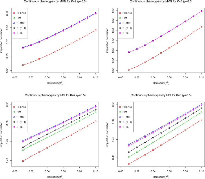
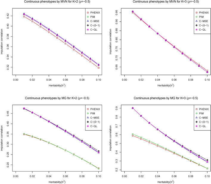
We apply our method with three typical loss functions C-MSE, C-(0–1), C-QL and two comparsion methods (PHENIX and PIM) to each scenario of the simulated data sets to infer the missing phenotypes. The results are shown in Fig. 1 for the correlation of the phenotypes $\rho$ at 0.5 and Fig. 2 for the correlation of the phenotypes $\rho$ at $-$0.5 varying the heritability of the phenotypes, i.e., the relative contributions of the genetic variant from zero to 0.1. The overall pattern from these two figures shows that our methods outperform or have similar performance to the other two methods over the range of heritability. Specifically, the performance of all methods is similar under the multivariate normal assumption and our methods outperform the other two methods for the multivariate gamma assumption, where they have incorrect distribution assumptions for the PIM and PHENIX methods. It shows that our methods are more flexible than these two methods, i.e., placing no restrictions on the distribution of the data.

Fig. 1.

The imputation correlation of five methods (PHNIX, PIM, C-MSE, C-(0–1) and C-QL) for phenotype values ($n=1000$) simulated from multivariate normal distribution (top) and multivariate gamma distribution (bottom) at $\rho =0.5$ with varied heritability of the traits by adjusting the relative contributions of genetic variants where the correlation of the imputed values with the true values is plotted on the y axis for each method

Fig. 2.

The imputation correlation of five methods (PHNIX, PIM, C-MSE, C-(0–1) and C-QL) for phenotype values ($n=1000$) simulated from multivariate normal distribution (top) and multivariate gamma distribution (bottom) at $\rho =-0.5$ with varied heritability of the traits by adjusting the relative contributions of genetic variants where the correlation of the imputed values with the true values is plotted on the y axis for each method

As heritability increases, the imputation correlation seems to increase slightly for positive correlation of phenotypes $\rho =0.5$ and decrease slightly for negative correlation of phenotypes $\rho =-0.5$. This occurs because the overall correlations between phenotypes are a mixture of genetic (g) and correlations ($\rho$). For positive $\rho$, the overall correlations increase as heritability increases and weaken as heritability increases for negative $\rho$ because the genetics and correlations tend to cancel each other out.

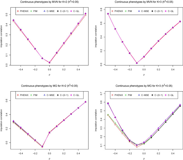
Figure 3 presents the results of imputation correlation comparisons among the five methods when the heritability $h^2$ is held constant (0.05) but $\rho$ is varied from $-0.5$ to 0.5. As the correlation $\rho$ increases from $-$0.5 to 0, the imputation correlation of all methods decreases, but then increases again as the correlation $\rho$ increases from 0 to 0.5. The reason is that it makes the correlation among phenotypes weak as $\rho$ increases from negative to zero and strong as $\rho$ increases from zero to 0.5, while the point estimates of the missing phenotypes depend on the strength of the correlation among phenotypes. Figures 1, 2, and 3 show that our methods seem to perform roughly equally well or better than the other two methods. From these three figures, we can also see that method C-(0–1) is slightly worse than methods C-MSE and C-QL. Both C-MSE and C-QL have similar imputation correlations. The reason is that the definition of the 0–1 loss function is too strict. In summary, our method remained the best-performing approach regardless of whether the phenotypes followed a multivariate normal or multivariate gamma (MG) distribution, even when the correlations among phenotypes varied.

Fig. 3.

The imputation correlation of five methods (PHNIX, PIM, C-MSE, C-(0–1) and C-QL) for phenotype values ($n=1000$) simulated from multivariate normal distribution (top) and multivariate gamma distribution (bottom) at $h^2=0.05$ is evaluated across a range of positive and negative correlations among phenotypes. The y-axis represents the correlation between the imputed and true values for each method

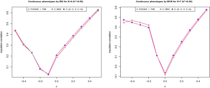
When we increase the number of phenotypes to $K=4$ and $K=7$ (Fig. 4) or even a broader range of phenotypes from $K=4$ to $K=15$ (Supplementary Figure 1), our methods have similar or better performance than PIM and PHENIX for most of K. Specifically, when four phenotypes are generated from multivariate gamma distributions, our method performs similarly to PIM and PHENIX when negative correlations among the phenotypes are present, but outperforms both PIM and PHENIX when positive correlations exists among the phenotypes. When seven phenotypes are generated from multivariate normal distributions, our method performs better than PIM and PHENIX in the presence of positive correlations among the phenotype, while PIM and PHENIX only outperform our method when the negative correlations among the phenotypes were in the range of $-$0.4 to $-$0.2.

Fig. 4.

The imputation correlation of five methods (PHENIX, PIM, C-MSE, C-(0–1) and C-QL) for phenotype values ($n=1000$) simulated from a multivariate gamma distribution (left) and multivariate normal distribution (right) at $h^2=0.05$ with varying numbers and correlations of phenotypes is presented. The y-axis shows the correlation between the imputed and true values for each imputation method

Our method performs better than or similarly to PIM and PHENIX when the number of phenotypes ranges from 5 to 14 (Supplementary Figure 1). PHENIX and PIM only outperform our method when the number of phenotypes is 4 or 15. The phenotypes in Supplementary Figure 1 are generated from multivariate normal distributions, which satisfy the key assumptions of PHENIX and PIM. However, when phenotypes are generated from multivariate gamma distributions or a mixture of multivariate normal, multivariate gamma, and beta distributions, the performance of PHENIX and PIM declines even further, as these scenarios violate the key multivariate normal assumption required for their effectiveness (data not shown).

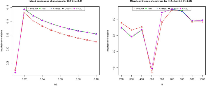
When a mixture distribution is employed to generate seven phenotypes including two multivariate normal phenotypes, two multivariate gamma distributions phenotypes, and three beta distributions phenotypes (Fig. 5), our methods consistently outperform PHENIX as heritability varies from 0.02 to 0.1. In addition, our methods perform better than PHENIX when the sample size increases from 500 to 1000. PHENIX only outperforms our methods when the heritability is low (i.e. 0.01) or when the sample size is small (200, 300, or 400). The performance of PHENIX declines with phenotypes generated from a mixture distribution, primarily because this distribution violates the assumptions of multivariate normal which is required for its effectiveness. The PIM method performs similarly to our method because it leverages the correlation structure to impute phenotypes with missing data. However, the normality assumption can impact the performance of PIM when the actual distribution of the data deviates from the multivariate normality as shown in Figs. 1, 2 and 3, where phenotypes are generated from multivariate gamma distributions.

Fig. 5.

The imputation correlation of five methods (PHENIX, PIM, C-MSE, C-(0–1) and C-QL) for phenotype values simulated from a mixture of multivariate normal, beta, and gamma distributions is evaluated for varying $h^2$ when $n=1000$, and varying sample size from $n=200$ to 1000. The y-axis represents the correlation between the imputed and true values for each method

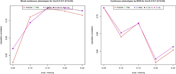
When considering different missing rates in phenotypes, our methods outperform the PHENIX method at most missing rates for phenotypes generated from the mixture distribution, except at $0.1$ missing rate when phenotypes are generated from a mixture distribution (comprising two multivariate normal phenotypes, two multivariate gamma phenotypes, and three beta phenotypes). Conversely, our methods consistently outperform PHENIX across all missing rates when the phenotypes are generated from a multivariate normal distribution. The strong performance of our methods across different missing rates demonstrates their robustness and general applicability (Fig. 6).

Fig. 6.

The imputation correlation of five methods (PHENIX, PIM, C-MSE, C-(0–1) and C-QL) for phenotype values ($n=1000$) simulated from a mixture of multivariate normal, beta, and gamma distributions. In this plot, the y-axis represents the correlation of the imputed values with the true values, while the x-axis represents the proportion of missingness in phenotypes, varying from 0.05 to 0.25

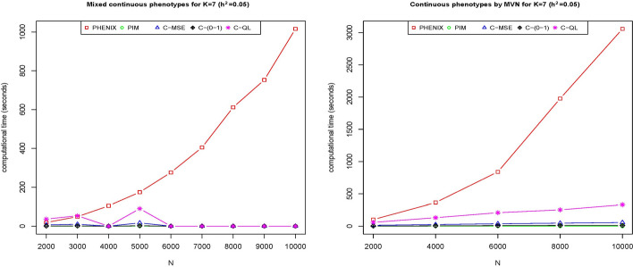
Figure 7 presents the computational time (in seconds) for our methods and the two existing methods, PIM and PHENIX, with varying sample sizes from 2,000 to 10,000. For seven phenotypes with a sample size of 10,000, both PIM and our methods complete the imputation in less than 100 s using an HP laptop with a 1.70 GHz CPU and 32.0 GB of RAM. PIM along with our C-MSE and C-(0–1) methods, are the most efficient, followed by our C-QL method. In contrast, PHENIX is computationally intensive.

Fig. 7.

The computation time of five methods (PHENIX, PIM, C-MSE, C-(0–1) and C-QL) for phenotype values simulated from a multivariate normal and a mixture of multivariate normal, beta, and gamma distributions for varying sample size when $h^2=0.05$ and $\rho =0.5$, where the y-axis represents the computation time in seconds and x-axis represents the sample size (N)

As we know that large sample size can help us achieve the desired statistical power, the primary purpose of imputation is to fill in the remaining missing phenotypes, helping to maximize the effective sample size to improve power in GWASs. As such, it is important to show that our approach leads to effective statistical tests by using one phenotypes at a time or by using multiple phenotypes simultaneously in association tests. It is a wide consensus that the data after imputation can increase power in association tests.

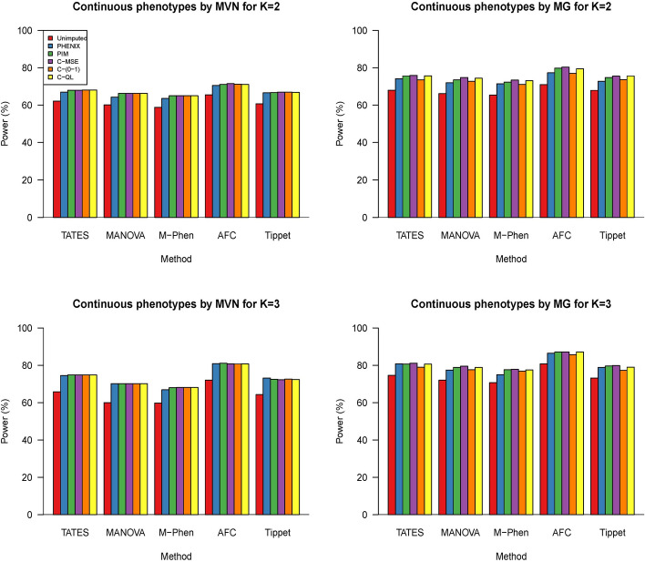
In Fig. 8, we use simulated phenotype and genotype data (sample size $n=500$) to evaluate power for detecting associations using five different multiple-phenotype test methods TATES [14], MANOVA [15], M-Phen [16], AFC [17] and Tippet [18] where we set $\rho =0.3$ and $h^2=0.01$. We found that the imputed data could lead to an increase in power and our methods (C-MSE, C-(0–1), and C-QL) have similar power with two other comparative methods under scenario 1. Under scenario 2, using C-MSE and C-QL leads to the highest power compared to other methods. This may be because the basic assumption of PHNIX and PIM is against the distribution assumption of scenario 2 and C-(0–1) has a relatively strict loss function. Compared to imputed data, tests based on unimputed data have a loss of power, which is consistent with the fact that the use of imputation can increase the power of GWAS. In summary, the tests based on C-QL and C-MSE achieve the best power.

Fig. 8.

Bar charts of the power for the five different multiple phenotype association methods (TATES, MANOVA, M-Phen, AFC and Tippet) based on different imputation options

The type I error evaluation from our simulation studies confirmed that violating normality assumptions inflates type I error rates in genetic association tests for existing methods, PIM and PHENIX. Both PIM and PHENIX show inflated type I error rates when seven phenotypes are generated from multivariate gamma distributions, with even more severe inflation when the phenotypes are generated from a mixture distribution (two multivariate normal phenotypes, two multivariate gamma phenotypes, and three beta phenotypes). In contrast, the type I error rates for all methods remain well-controlled when phenotypes are unimputed or imputed using our proposed methods (Table 1).

Table 1.

The type I error rates of genetic association tests with phenotypes imputed with different methods. ($\alpha$=0.05, 95$\%$ confidence interval of $\alpha$: (0.0362, 0.0638); heritability $h^2=0;$ correlation of phenotypes $\rho$ =0.5; 1000 replicated samples; sample size $n=1000$)

Dist. $_{}^1$	Association tests	Unimputed	PHENIX	PIM	C-MSE	C-(0–1)	C-QL
MVN	TATES	0.055	0.057	0.045	0.040	0.052	0.043
	MANOVA	0.049	0.036	0.043	0.038	0.037	0.042
	M-Phen	0.051	0.044	0.059	0.060	0.057	0.062
	AFC	0.055	0.046	0.037	0.043	0.058	0.061
	Tippel	0.049	0.061	0.055	0.056	0.049	0.044
MG	TATES	0.051	$\mathbf{0.066}$	$\mathbf{0.071}$	0.039	0.053	0.060
	MANOVA	0.054	$\mathbf{0.065}$	$\mathbf{0.073}$	0.051	0.047	0.043
	M-Phen	0.045	$\mathbf{0.080}$	$\mathbf{0.075}$	0.044	0.050	0.053
	AFC	0.055	$\mathbf{0.065}$	$\mathbf{0.063}$	0.047	0.056	0.059
	Tippel	0.050	$\mathbf{0.074}$	$\mathbf{0.077}$	0.060	0.054	0.039
Mixed	TATES	0.055	$\mathbf{0.077}$	$\mathbf{0.085}$	0.037	0.042	0.045
	MANOVA	0.049	$\mathbf{0.079}$	$\mathbf{0.084}$	0.056	0.052	0.061
	M-Phen	0.049	$\mathbf{0.088}$	$\mathbf{0.079}$	0.057	0.061	0.060
	AFC	0.036	$\mathbf{0.068}$	$\mathbf{0.070}$	0.048	0.060	0.054
	Tippel	0.048	$\mathbf{0.090}$	$\mathbf{0.085}$	0.056	0.061	0.053

$_{}^1$Dist.: Phenotypes’ distributions; MVN: 7 phenotypes follow multivariate normal distribution (MVN); MG: 7 phenotypes follow multivariate gamma distribution; Mixed: 7 phenotypes follow a mixture of multivariate normal, beta, and gamma distributions

Bold values indicate inflated type I errors

To compare the performance of our methods with the Gaussian copula method using the EM algorithm (Copula-EM) for phenotype imputation [12], three and seven phenotypes are generated from multivariate normal distributions and multivariate gamma distributions, respectively. When the phenotypes follow multivariate normal distributions, our methods outperform Copula-EM consistently for the three-phenotype case and show even greater improvement when the sample size is 100 for the seven-phenotype case. When phenotypes follow multivariate gamma distributions, our methods outperform Copula-EM at larger sample sizes, such as 500 for seven phenotypes or 600 for three phenotypes. This indicates that our methods are particularly robust when dealing with multivariate normal distributions, excelling in both small and large sample sizes. Although our methods are effective for non-normal data, they require a sufficiently large sample size to maintain their advantage over Copula-EM in these situations (Supplementary Figure 2).

Application to the COPDGene

Chronic obstructive pulmonary disease (COPD) is one of the most common lung diseases characterized by long-term poor airflow and is a major public health problem [19]. The COPDGene Study is a multicenter genetic and epidemiologic investigation to study COPD [20]. This study is sufficiently large and appropriately designed for genome-wide association analysis of COPD. In this study, we considered more than 5000 non-Hispanic White (NHW) participants who completed a detailed protocol, including questionnaires, pre- and postbronchodilator spirometry, high-resolution CT scanning of the chest, exercise capacity (assessed by six-minute walk distance), and blood samples for genotyping. The participants were genotyped using the Illumina OmniExpress platform. The genotype data have gone through standard quality-control procedures for genome-wide association analysis detailed at http://www.copdgene.org/sites/default/files/GWAS_QC_Methodology_20121115.pdf. Variants with MAF$<1\%$ were excluded in the data set.

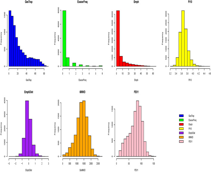
Based on the literature studies of COPD [21, 22], we selected seven key quantitative COPD-related phenotypes, including FEV1 (% predicted FEV1), emphysema (Emph), emphysema distribution (EmphDist), gas trapping (GasTrap), airway wall area (Pi10), exacerbation frequency (ExacerFreq), six-minute walk distance (6MWD), and 4 covariates, including BMI, age, pack-years (PackYear), and sex. EmphDist is the ratio of emphysema at −950 HU in the upper 1/3 of lung fields compared to the lower 1/3 of lung fields where we performed a log transformation on EmphDist in the following analysis, referred to [21]. A complete set of 6576 individuals was used in the analyses. The missing rates of the 7 COPD-related phenotypes are 13.17% (GasTrap), 0% (ExacerFreq), 5.89% (Emph), 6.81% (Pi10), 8.06% (EmphDist), 1.58% (6MWD) and 0.39% (% predicted FEV1). In Fig. 9, the histograms of the seven key quantitative COPD-related phenotypes show distinct marginal distributions. Pi10, EmphDist, and 6MWD approximate a normal distribution. GasTrap resembles a chi-square distribution, while ExacerFreq and Emph fit a gamma distribution. FEV1, on the other hand, follows a beta distribution. These varied distributions highlight the need for phenotype imputation with copula method in a realistic setting, as it allows for more accurate modeling of the complex dependencies between phenotypes with differing marginal distributions.

Fig. 9.

Histograms of seven key quantitative COPD-related phenotypes

To evaluate the performance of our proposed methods on a real data set, we applied all 5 methods (TATES, MANOVA, M-Phen, AFC, and Tippet) to the COPDGene of the NHW population to carry out GWAS of COPD-related phenotypes (imputed phenotypes). In the analysis, participants with missing data for any genotypic variants were excluded. We first imputed the missing phenotypes and then adjusted each of the 7 phenotypes for the 4 covariates using linear models. We calculated the p-value based on these 5 methods for the adjusted phenotypes. To identify SNPs associated with the phenotypes, we adopted the commonly used genome-wide significance level $5\times {10}^{-8}$. The results were summarized in Tables 2, 3, 4, 5, and there were a total 14 SNPs in each table. All 14 SNPs had previously been reported to be associated with COPD by eligible studies [23–35] and [36]. From these tables, we can see that the p value of unimputed data is always larger than the p value of each imputed dataset. Among the five imputation methods, our method is the imputation method with either the smallest p value or having a similar p value as the imputation method with the least p value in most of the scenarios. PHENIX has a similar performance as ours in some scenarios (Table 6).

Table 2.

The corresponding p values of significant SNPs of MANOVA in the analysis of COPDGene using different imputation methods

Chr:bp$_{}^1$	SNP$_{}^2$	Unimputed	PHENIX	PIM	C-MSE	C-(0–1)	C-QL
4:145431497	rs1512282	$1.69E-9$	$\mathbf{1.47}\mathbf{E}-\mathbf{11}$	$1.96E-11$	$2.40E-11$	$2.42E-11$	$2.40E-11$
4:145434744	rs1032297	$6.52E-14$	$4.71E-15$	$6.93E-15$	$\mathbf{2.02}\mathbf{E}-\mathbf{15}$	$2.12E-15$	$\mathbf{2.02}\mathbf{E}-\mathbf{15}$
4:145474473	rs1489759	$1.11E-16$	$4.96E-16$	$2.08E-16$	$\mathbf{7.46}\mathbf{E}-\mathbf{17}$	$7.90E-17$	$7.47E-17$
4:145485738	rs1980057	$6.68E-17$	$6.00E-17$	$2.48E-17$	$\mathbf{8.00}\mathbf{E}-\mathbf{18}$	$8.46E-18$	$\mathbf{8.00}\mathbf{E}-\mathbf{18}$
4:145485915	rs7655625	$7.12E-17$	$1.39E-16$	$5.95E-17$	$\mathbf{2.16}\mathbf{E}-\mathbf{17}$	$2.28E-17$	$\mathbf{2.16}\mathbf{E}-\mathbf{17}$
15:78882925	rs16969968	$1.32E-11$	$4.49E-14$	$2.71E-14$	$1.51E-14$	$\mathbf{1.41}\mathbf{E}-\mathbf{14}$	$1.51E-14$
15:78894339	rs1051730	$1.41E-11$	$4.44E-14$	$2.74E-14$	$1.40E-14$	$\mathbf{1.36}\mathbf{E}-\mathbf{14}$	$1.40E-14$
15:78898723	rs12914385	$1.76E-12$	$1.20E-14$	$3.44E-15$	$1.85E-15$	$\mathbf{1.70}\mathbf{E}-\mathbf{15}$	$1.85E-15$
15:78911181	rs8040868	$2.74E-12$	$5.78E-15$	$2.11E-15$	$1.73E-15$	$\mathbf{1.61}\mathbf{E}-\mathbf{15}$	$1.73E-15$
15:78878541	rs951266	$1.77E-11$	$9.20E-14$	$6.88E-14$	$3.03E-14$	$\mathbf{2.95}\mathbf{E}-\mathbf{14}$	$3.03E-14$
15:78806023	rs8034191	$2.14E-10$	$1.03E-12$	$\mathbf{1.70}\mathbf{E}-\mathbf{13}$	$2.25E-13$	$2.19E-13$	$2.25E-13$
15:78851615	rs2036527	$3.99E-10$	$4.63E-13$	$\mathbf{1.04}\mathbf{E}-\mathbf{13}$	$1.09E-13$	$1.06E-13$	$1.09E-13$
15:78826180	rs931794	$2.35E-10$	$7.92E-13$	$\mathbf{1.75}\mathbf{E}-\mathbf{13}$	$2.22E-13$	$2.17E-13$	$2.22E-13$
15:78740964	rs2568494	$1.05E-7$	$2.63E-10$	$2.41E-10$	$1.94E-10$	$\mathbf{1.89}\mathbf{E}-\mathbf{10}$	$1.94E-10$

$_{}^1$Chr:bp denotes chromosome and base pair position

$_{}^2$SNP denotes Single Nucleotide Polymorphism

$_{}^3$Bold-faced value indicates the smallest p value based on unimputed and imputed data

Table 3.

The corresponding p values of significant SNPs of TATES in the analysis of COPDGene using different imputation methods

Chr:bp$_{}^1$	SNP$_{}^2$	Unimputed	PHENIX	PIM	C-MSE	C-(0–1)	C-QL
4:145431497	rs1512282	$5.77E-9$	$1.27E-9$	$1.41E-9$	$\mathbf{5.13}\mathbf{E}-\mathbf{10}$	$5.19E-10$	$\mathbf{5.13}\mathbf{E}-\mathbf{10}$
4:145434744	rs1032297	$6.22E-13$	$1.20E-12$	$3.50E-13$	$\mathbf{8.17}\mathbf{E}-\mathbf{14}$	$8.59E-14$	$\mathbf{8.17}\mathbf{E}-\mathbf{14}$
4:145474473	rs1489759	$2.52E-16$	$4.09E-15$	$7.08E-16$	$<\mathbf{1.00}\mathbf{E}-\mathbf{16}$	$<\mathbf{1.00}\mathbf{E}-\mathbf{16}$	$<\mathbf{1.00}\mathbf{E}-\mathbf{16}$
4:145485738	rs1980057	$9.35E-17$	$6.82E-16$	$<\mathbf{1.00}\mathbf{E}-\mathbf{16}$	$<\mathbf{1.00}\mathbf{E}-\mathbf{16}$	$<\mathbf{1.00}\mathbf{E}-\mathbf{16}$	$<\mathbf{1.00}\mathbf{E}-\mathbf{16}$
4:145485915	rs7655625	$1.64E-16$	$1.36E-15$	$<\mathbf{1.00}\mathbf{E}-\mathbf{16}$	$<\mathbf{1.00}\mathbf{E}-\mathbf{16}$	$<\mathbf{1.00}\mathbf{E}-\mathbf{16}$	$<\mathbf{1.00}\mathbf{E}-\mathbf{16}$
15:78882925	rs16969968	$2.98E-8$	$\mathbf{9.90}\mathbf{E}-\mathbf{11}$	$6.26E-10$	$1.88E-10$	$1.87E-10$	$1.88E-10$
15:78894339	rs1051730	$2.63E-8$	$\mathbf{6.91}\mathbf{E}-\mathbf{11}$	$4.30E-10$	$1.26E-10$	$1.27E-10$	$1.26E-10$
15:78898723	rs12914385	$5.14E-10$	$\mathbf{1.18}\mathbf{E}-\mathbf{12}$	$3.03E-12$	$1.29E-12$	$1.24E-12$	$1.29E-12$
15:78911181	rs8040868	$2.40E-9$	$\mathbf{1.89}\mathbf{E}-\mathbf{12}$	$1.15E-11$	$4.70E-12$	$4.52E-12$	$4.70E-12$
15:78878541	rs951266	$5.17E-8$	$\mathbf{1.91}\mathbf{E}-\mathbf{10}$	$1.18E-9$	$3.54E-10$	$3.54E-10$	$3.54E-10$
15:78806023	rs8034191	$1.02E-7$	$\mathbf{5.77}\mathbf{E}-\mathbf{10}$	$1.87E-9$	$9.48E-10$	$9.49E-10$	$9.48E-10$
15:78851615	rs2036527	$1.56E-7$	$\mathbf{4.06}\mathbf{E}-\mathbf{10}$	$2.07E-9$	$7.45E-10$	$7.44E-10$	$7.45E-10$
15:78826180	rs931794	$1.18E-7$	$\mathbf{4.37}\mathbf{E}-\mathbf{10}$	$2.18E-9$	$9.49E-10$	$9.49E-10$	$9.49E-10$
15:78740964	rs2568494	$2.88E-5$	$5.85E-7$	$1.37E-6$	$4.90E-7$	$\mathbf{4.77}\mathbf{E}-\mathbf{7}$	$4.90E-7$

$_{}^1$Chr:bp denotes chromosome and base pair position

$_{}^2$SNP denotes Single Nucleotide Polymorphism

Bold values indicate the smallest p value for the genetic association tests using imputed and unimputed data for each SNP

Table 4.

The corresponding p values of significant SNPs of M-Phen in the analysis of COPDGene using different imputation methods

Chr:bp$_{}^1$	SNP$_{}^2$	Unimputed	PHENIX	PIM	C-MSE	C-(0–1)	C-QL
4:145431497	rs1512282	$1.03E-9$	$\mathbf{7.33}\mathbf{E}-\mathbf{12}$	$9.15E-12$	$1.11E-11$	$1.12E-11$	$1.11E-11$
4:145434744	rs1032297	$7.69E-14$	$7.44E-15$	$7.22E-15$	$\mathbf{2.55}\mathbf{E}-\mathbf{15}$	$2.66E-15$	$\mathbf{2.55}\mathbf{E}-\mathbf{15}$
4:145474473	rs1489759	$1.22E-16$	$4.44E-16$	$\mathbf{1.11}\mathbf{E}-\mathbf{16}$	$\mathbf{1.11}\mathbf{E}-\mathbf{16}$	$\mathbf{1.11}\mathbf{E}-\mathbf{16}$	$\mathbf{1.11}\mathbf{E}-\mathbf{16}$
4:145485738	rs1980057	$8.14E-17$	$1.11E-16$	$<\mathbf{1.00}\mathbf{E}-\mathbf{16}$	$<\mathbf{1.00}\mathbf{E}-\mathbf{16}$	$<\mathbf{1.00}\mathbf{E}-\mathbf{16}$	$<\mathbf{1.00}\mathbf{E}-\mathbf{16}$
4:145485915	rs7655625	$9.13E-17$	$1.11E-16$	$<\mathbf{1.00}\mathbf{E}-\mathbf{16}$	$<\mathbf{1.00}\mathbf{E}-\mathbf{16}$	$<\mathbf{1.00}\mathbf{E}-\mathbf{16}$	$<\mathbf{1.00}\mathbf{E}-\mathbf{16}$
15:78882925	rs16969968	$7.84E-12$	$3.26E-14$	$2.20E-14$	$1.10E-14$	$\mathbf{1.08}\mathbf{E}-\mathbf{14}$	$1.10E-14$
15:78894339	rs1051730	$8.16E-12$	$3.10E-14$	$2.02E-14$	$9.44E-15$	$\mathbf{9.33}\mathbf{E}-\mathbf{15}$	$9.44E-15$
15:78898723	rs12914385	$1.48E-12$	$1.59E-14$	$4.55E-15$	$2.11E-15$	$\mathbf{2.00}\mathbf{E}-\mathbf{15}$	$2.11E-15$
15:78911181	rs8040868	$2.59E-12$	$6.99E-15$	$2.89E-15$	$2.11E-15$	$\mathbf{2.00}\mathbf{E}-\mathbf{15}$	$2.11E-15$
15:78878541	rs951266	$1.02E-11$	$6.71E-14$	$5.87E-14$	$2.24E-14$	$\mathbf{2.20}\mathbf{E}-\mathbf{14}$	$2.24E-14$
15:78806023	rs8034191	$7.74E-11$	$4.17E-13$	$\mathbf{7.84}\mathbf{E}-\mathbf{14}$	$9.41E-14$	$9.26E-14$	$9.41E-14$
15:78851615	rs2036527	$1.77E-10$	$2.69E-13$	$6.29E-14$	$6.04E-14$	$\mathbf{5.94}\mathbf{E}-\mathbf{14}$	$6.04E-14$
15:78826180	rs931794	$9.09E-11$	$2.99E-13$	$\mathbf{7.59}\mathbf{E}-\mathbf{14}$	$9.14E-14$	$9.00E-14$	$9.14E-14$
15:78740964	rs2568494	$4.23E-8$	$8.91E-11$	$1.01E-10$	$7.35E-11$	$\mathbf{7.21}\mathbf{E}-\mathbf{11}$	$7.36E-11$

$_{}^1$Chr:bp denotes chromosome and base pair position

$_{}^2$SNP denotes Single Nucleotide Polymorphism

Bold values indicate the smallest p value for the genetic association tests using imputed and unimputed data for each SNP

Table 5.

The corresponding p values of significant SNPs of AFC in the analysis of COPDGene using different imputation methods

Chr:bp$_{}^1$	SNP$_{}^2$	Unimputed	PHENIX	PIM	C-MSE	C-(0–1)	C-QL
4:145431497	rs1512282	$1.1\times {10}^{-8}$	$<\mathbf{1.00}\mathbf{E}-\mathbf{16}$	$<\mathbf{1.00}\mathbf{E}-\mathbf{16}$	$<\mathbf{1.00}\mathbf{E}-\mathbf{16}$	$<\mathbf{1.00}\mathbf{E}-\mathbf{16}$	$<\mathbf{1.00}\mathbf{E}-\mathbf{16}$
4:145434744	rs1032297	$<\mathbf{1.00}\mathbf{E}-\mathbf{16}$	$<\mathbf{1.00}\mathbf{E}-\mathbf{16}$	$<\mathbf{1.00}\mathbf{E}-\mathbf{16}$	$<\mathbf{1.00}\mathbf{E}-\mathbf{16}$	$<\mathbf{1.00}\mathbf{E}-\mathbf{16}$	$<\mathbf{1.00}\mathbf{E}-\mathbf{16}$
4:145474473	rs1489759	$<\mathbf{1.00}\mathbf{E}-\mathbf{16}$	$<\mathbf{1.00}\mathbf{E}-\mathbf{16}$	$<\mathbf{1.00}\mathbf{E}-\mathbf{16}$	$<\mathbf{1.00}\mathbf{E}-\mathbf{16}$	$<\mathbf{1.00}\mathbf{E}-\mathbf{16}$	$<\mathbf{1.00}\mathbf{E}-\mathbf{16}$
4:145485738	rs1980057	$<\mathbf{1.00}\mathbf{E}-\mathbf{16}$	$<\mathbf{1.00}\mathbf{E}-\mathbf{16}$	$<\mathbf{1.00}\mathbf{E}-\mathbf{16}$	$<\mathbf{1.00}\mathbf{E}-\mathbf{16}$	$<\mathbf{1.00}\mathbf{E}-\mathbf{16}$	$<\mathbf{1.00}\mathbf{E}-\mathbf{16}$
4:145485915	rs7655625	$<\mathbf{1.00}\mathbf{E}-\mathbf{16}$	$<\mathbf{1.00}\mathbf{E}-\mathbf{16}$	$<\mathbf{1.00}\mathbf{E}-\mathbf{16}$	$<\mathbf{1.00}\mathbf{E}-\mathbf{16}$	$<\mathbf{1.00}\mathbf{E}-\mathbf{16}$	$<\mathbf{1.00}\mathbf{E}-\mathbf{16}$
15:78882925	rs16969968	$<\mathbf{1.00}\mathbf{E}-\mathbf{16}$	$<\mathbf{1.00}\mathbf{E}-\mathbf{16}$	$<\mathbf{1.00}\mathbf{E}-\mathbf{16}$	$<\mathbf{1.00}\mathbf{E}-\mathbf{16}$	$<\mathbf{1.00}\mathbf{E}-\mathbf{16}$	$<\mathbf{1.00}\mathbf{E}-\mathbf{16}$
15:78894339	rs1051730	$<\mathbf{1.00}\mathbf{E}-\mathbf{16}$	$<\mathbf{1.00}\mathbf{E}-\mathbf{16}$	$<\mathbf{1.00}\mathbf{E}-\mathbf{16}$	$<\mathbf{1.00}\mathbf{E}-\mathbf{16}$	$<\mathbf{1.00}\mathbf{E}-\mathbf{16}$	$<\mathbf{1.00}\mathbf{E}-\mathbf{16}$
15:78898723	rs12914385	$<\mathbf{1.00}\mathbf{E}-\mathbf{16}$	$<\mathbf{1.00}\mathbf{E}-\mathbf{16}$	$<\mathbf{1.00}\mathbf{E}-\mathbf{16}$	$<\mathbf{1.00}\mathbf{E}-\mathbf{16}$	$<\mathbf{1.00}\mathbf{E}-\mathbf{16}$	$<\mathbf{1.00}\mathbf{E}-\mathbf{16}$
15:78911181	rs8040868	$<\mathbf{1.00}\mathbf{E}-\mathbf{16}$	$<\mathbf{1.00}\mathbf{E}-\mathbf{16}$	$<\mathbf{1.00}\mathbf{E}-\mathbf{16}$	$<\mathbf{1.00}\mathbf{E}-\mathbf{16}$	$<\mathbf{1.00}\mathbf{E}-\mathbf{16}$	$<\mathbf{1.00}\mathbf{E}-\mathbf{16}$
15:78878541	rs951266	$<\mathbf{1.00}\mathbf{E}-\mathbf{16}$	$<\mathbf{1.00}\mathbf{E}-\mathbf{16}$	$<\mathbf{1.00}\mathbf{E}-\mathbf{16}$	$<\mathbf{1.00}\mathbf{E}-\mathbf{16}$	$<\mathbf{1.00}\mathbf{E}-\mathbf{16}$	$<\mathbf{1.00}\mathbf{E}-\mathbf{16}$
15:78806023	rs8034191	$1.40\times {10}^{-8}$	$<\mathbf{1.00}\mathbf{E}-\mathbf{16}$	$<\mathbf{1.00}\mathbf{E}-\mathbf{16}$	$<\mathbf{1.00}\mathbf{E}-\mathbf{16}$	$<\mathbf{1.00}\mathbf{E}-\mathbf{16}$	$<\mathbf{1.00}\mathbf{E}-\mathbf{16}$
15:78851615	rs2036527	$2.90\times {10}^{-8}$	$<\mathbf{1.00}\mathbf{E}-\mathbf{16}$	$<\mathbf{1.00}\mathbf{E}-\mathbf{16}$	$<\mathbf{1.00}\mathbf{E}-\mathbf{16}$	$<\mathbf{1.00}\mathbf{E}-\mathbf{16}$	$<\mathbf{1.00}\mathbf{E}-\mathbf{16}$
15:78826180	rs931794	$6.30\times {10}^{-8}$	$<\mathbf{1.00}\mathbf{E}-\mathbf{16}$	$<\mathbf{1.00}\mathbf{E}-\mathbf{16}$	$<\mathbf{1.00}\mathbf{E}-\mathbf{16}$	$<\mathbf{1.00}\mathbf{E}-\mathbf{16}$	$<\mathbf{1.00}\mathbf{E}-\mathbf{16}$
15:78740964	rs2568494	$5.00\times {10}^{-6}$	$5.00\times {10}^{-7}$	$8.00\times {10}^{-7}$	$<\mathbf{1.00}\mathbf{E}-\mathbf{16}$	$<\mathbf{1.00}\mathbf{E}-\mathbf{16}$	$<\mathbf{1.00}\mathbf{E}-\mathbf{16}$

$_{}^1$Chr:bp denotes chromosome and base pair position

$_{}^2$SNP denotes Single Nucleotide Polymorphism

Bold values indicate the smallest p value for the genetic association tests using imputed and unimputed data for each SNP

Table 6.

The corresponding p values of significant SNPs of Tippet in the analysis of COPDGene for different imputation methods

Chr:bp$_{}^1$	SNP$_{}^2$	Unimputed	PHENIX	PIM	C-MSE	C-(0–1)	C-QL
4:145431497	rs1512282	$8.00\times {10}^{-9}$	$<\mathbf{1.00}\mathbf{E}-\mathbf{16}$	$<\mathbf{1.00}\mathbf{E}-\mathbf{16}$	$<\mathbf{1.00}\mathbf{E}-\mathbf{16}$	$<\mathbf{1.00}\mathbf{E}-\mathbf{16}$	$<\mathbf{1.00}\mathbf{E}-\mathbf{16}$
4:145434744	rs1032297	$<\mathbf{1.00}\mathbf{E}-\mathbf{16}$	$<\mathbf{1.00}\mathbf{E}-\mathbf{16}$	$<\mathbf{1.00}\mathbf{E}-\mathbf{16}$	$<\mathbf{1.00}\mathbf{E}-\mathbf{16}$	$<\mathbf{1.00}\mathbf{E}-\mathbf{16}$	$<\mathbf{1.00}\mathbf{E}-\mathbf{16}$
4:145474473	rs1489759	$<\mathbf{1.00}\mathbf{E}-\mathbf{16}$	$<\mathbf{1.00}\mathbf{E}-\mathbf{16}$	$<\mathbf{1.00}\mathbf{E}-\mathbf{16}$	$<\mathbf{1.00}\mathbf{E}-\mathbf{16}$	$<\mathbf{1.00}\mathbf{E}-\mathbf{16}$	$<\mathbf{1.00}\mathbf{E}-\mathbf{16}$
4:145485738	rs1980057	$<\mathbf{1.00}\mathbf{E}-\mathbf{16}$	$<\mathbf{1.00}\mathbf{E}-\mathbf{16}$	$<\mathbf{1.00}\mathbf{E}-\mathbf{16}$	$<\mathbf{1.00}\mathbf{E}-\mathbf{16}$	$<\mathbf{1.00}\mathbf{E}-\mathbf{16}$	$<\mathbf{1.00}\mathbf{E}-\mathbf{16}$
4:145485915	rs7655625	$<\mathbf{1.00}\mathbf{E}-\mathbf{16}$	$<\mathbf{1.00}\mathbf{E}-\mathbf{16}$	$<\mathbf{1.00}\mathbf{E}-\mathbf{16}$	$<\mathbf{1.00}\mathbf{E}-\mathbf{16}$	$<\mathbf{1.00}\mathbf{E}-\mathbf{16}$	$<\mathbf{1.00}\mathbf{E}-\mathbf{16}$
15:78882925	rs16969968	$4.90\times {10}^{-8}$	$<\mathbf{1.00}\mathbf{E}-\mathbf{16}$	$<\mathbf{1.00}\mathbf{E}-\mathbf{16}$	$<\mathbf{1.00}\mathbf{E}-\mathbf{16}$	$<\mathbf{1.00}\mathbf{E}-\mathbf{16}$	$<\mathbf{1.00}\mathbf{E}-\mathbf{16}$
15:78894339	rs1051730	$4.20\times {10}^{-8}$	$<\mathbf{1.00}\mathbf{E}-\mathbf{16}$	$<\mathbf{1.00}\mathbf{E}-\mathbf{16}$	$<\mathbf{1.00}\mathbf{E}-\mathbf{16}$	$<\mathbf{1.00}\mathbf{E}-\mathbf{16}$	$<\mathbf{1.00}\mathbf{E}-\mathbf{16}$
15:78898723	rs12914385	$<\mathbf{1.00}\mathbf{E}-\mathbf{16}$	$<\mathbf{1.00}\mathbf{E}-\mathbf{16}$	$<\mathbf{1.00}\mathbf{E}-\mathbf{16}$	$<\mathbf{1.00}\mathbf{E}-\mathbf{16}$	$<\mathbf{1.00}\mathbf{E}-\mathbf{16}$	$<\mathbf{1.00}\mathbf{E}-\mathbf{16}$
15:78911181	rs8040868	$5.00\times {10}^{-9}$	$<\mathbf{1.00}\mathbf{E}-\mathbf{16}$	$<\mathbf{1.00}\mathbf{E}-\mathbf{16}$	$<\mathbf{1.00}\mathbf{E}-\mathbf{16}$	$<\mathbf{1.00}\mathbf{E}-\mathbf{16}$	$<\mathbf{1.00}\mathbf{E}-\mathbf{16}$
15:78878541	rs951266	$8.10\times {10}^{-8}$	$<\mathbf{1.00}\mathbf{E}-\mathbf{16}$	$<\mathbf{1.00}\mathbf{E}-\mathbf{16}$	$<\mathbf{1.00}\mathbf{E}-\mathbf{16}$	$<\mathbf{1.00}\mathbf{E}-\mathbf{16}$	$<\mathbf{1.00}\mathbf{E}-\mathbf{16}$
15:78806023	rs8034191	$1.70\times {10}^{-7}$	$<\mathbf{1.00}\mathbf{E}-\mathbf{16}$	$<\mathbf{1.00}\mathbf{E}-\mathbf{16}$	$<\mathbf{1.00}\mathbf{E}-\mathbf{16}$	$<\mathbf{1.00}\mathbf{E}-\mathbf{16}$	$<\mathbf{1.00}\mathbf{E}-\mathbf{16}$
15:78851615	rs2036527	$2.41\times {10}^{-7}$	$<\mathbf{1.00}\mathbf{E}-\mathbf{16}$	$<\mathbf{1.00}\mathbf{E}-\mathbf{16}$	$<\mathbf{1.00}\mathbf{E}-\mathbf{16}$	$<\mathbf{1.00}\mathbf{E}-\mathbf{16}$	$<\mathbf{1.00}\mathbf{E}-\mathbf{16}$
15:78826180	rs931794	$1.94\times {10}^{-7}$	$<\mathbf{1.00}\mathbf{E}-\mathbf{16}$	$<\mathbf{1.00}\mathbf{E}-\mathbf{16}$	$<\mathbf{1.00}\mathbf{E}-\mathbf{16}$	$<\mathbf{1.00}\mathbf{E}-\mathbf{16}$	$<\mathbf{1.00}\mathbf{E}-\mathbf{16}$
15:78740964	rs2568494	$3.42\times {10}^{-5}$	$3.00\times {10}^{-6}$	$2.00\times {10}^{-6}$	$<\mathbf{1.00}\mathbf{E}-\mathbf{16}$	$<\mathbf{1.00}\mathbf{E}-\mathbf{16}$	$<\mathbf{1.00}\mathbf{E}-\mathbf{16}$

$_{}^1$Chr:bp denotes chromosome and base pair position

$_{}^2$SNP denotes Single Nucleotide Polymorphism

Bold values indicate the smallest p value for the genetic association tests using imputed and unimputed data for each SNP

Discussion

Most of the recently developed imputation methods essentially focus on quantitative traits based on multivariate normal distribution. It is desirable to relax these restrictive assumptions in some natural way, allowing for features such as skewness and multimodality while simultaneously generalizing widely used and well-understood parametric models. Choosing an appropriate distribution to model these correlated traits is critical to the performance of these methods. In this paper, we used Gaussian Coupla to model the distribution of phenotype which is especially attractive for its flexibility. Based on the Gaussian Copula model assumption, we proposed three imputation methods under three different loss functions. We used a variety of simulation studies and applications to the lung study to compare the performance of our three methods with that of the existing methods. Our results show that our methods perform better than PIM and PHENIX which are two existing imputation methods.

Normalizing phenotypes before imputation can satisfy the requirement of certain imputation methods such as PHENIX and PIM, which require multivariate normal distributions. However, normalization can introduce artifacts, especially if the original data has complex, non-linear relationships. The transformation process may mask the true distribution and dependencies of the phenotypes, leading to biased imputation results. Imputing directly on the original data can preserve the inherent distribution and relationships within the data. Our proposed copula based method can handle diverse distributions without the need for normalization, potentially providing more accurate imputations.

Our proposed copula-based phenotype imputation method is not restricted to cases where missing data is independent and missing completely at random (MCAR). In fact, our method is also valid when the missingness is at random (MAR), where the probability of missingness may depend on observed phenotypes but not on the unobserved (missing) data itself. Our method leverages the Gaussian copula to capture the underlying correlation structure among the observed and missing phenotypes, which allows us to model the dependencies and impute missing values based on the observed data. In summary, the proposed copula-based imputation method is valid for MCAR and MAR missing data patterns.

For the missing not at random (MNAR) scenario, however, the method may face challenges, as it assumes that the missingness mechanism does not depend on unobserved values once conditioned on the observed data. Like most imputation methods, our method assumes that the missing data mechanism does not depend on the unobserved values in the case of MNAR, which typically requires additional assumptions or external information for phenotype imputation. Addressing phenotype imputation when the missingness is not at random (MNAR) will be the focus of our future work, as we aim to explore how to extend our copula-based phenotype imputation method to accommodate this more complex scenario.

The selection of an appropriate loss function is pivotal in determining the efficacy and performance of the proposed method. If the data is approximately normal and the goal is to minimize overall imputation error across the dataset, square loss (MSE) is recommended due to its balance between simplicity and effectiveness in handling continuous variables. If the data exhibit non-normal distribution or significant outliers, or there is a need to accurately estimate specific quantiles or extreme values, quantile loss could be more appropriate as it allows focusing on specific parts of the distribution. 0–1 loss is generally recommended for imputation tasks involving categorical variables due to its binary nature.

The proposed methods we discussed have implicitly been used to infer the last missing quantitative phenotype in the paper. If more quantitative missing phenotype occur in the same study, our methods can be easily extended to impute these missing phenotype one by one. We also note that we can readily impute qualitative phenotype based on the proposed Gaussian Copula model. On the other hand, qualitative phenotypes do often play an important role among all correlated phenotypes for some diseases in practice. Thus, taking full advantage of qualitative phenotypes to infer the missing quantitative phenotypes can increase the accuracy of imputation and thus improve the power for testing associations between phenotype and genetic variants.

We are currently exploring how to impute the qualitative phenotype under the Gaussian Copula model based on other loss functions and will report the results in the future.

Author contributions

Conceptualization: Qiuying Sha, Jianjun Zhang. Data curation: Qiuying Sha, Jianjun Zhang, Jane Zizhen Zhao, Samantha Gonzales. Formal analysis: Jianjun Zhang, Jane Zizhen Zhao, Samantha Gonzales. Investigation: Jianjun Zhang, Jane Zizhen Zhao, Samantha Gonzales. Methodology: Jianjun Zhang, Jane Zizhen Zhao, Xuexia Wang, Qiuying Sha. Project administration: Qiuying Sha. Supervision: Qiuying Sha. Writing - original draft: Jianjun Zhang, Jane Zizhen Zhao. Writing - review & editing: Jianjun Zhang, Jane Zizhen Zhao, Samantha Gonzales, Xuexia Wang, Qiuying Sha.

Funding

This study was partially supported by the FIU Diversity Center for Genomic Research grant (UG3HG013615, Principal Investigator: Xuexia Wang).

Availability of data and materials

The COPDGene data upon which these findings are based are available through the dbGaP study page for COPDGene: http://www.ncbi.nlm.nih.gov/projects/gap/cgi-bin/study.cgi?study_id=phs000179.v3.p2. There is a link from this page (Authorized Access Section) to dbGaP’s controlled access system that allows someone to request the data. The accession numbers for this data are phs000179/HMB and phs000179/DS-CS-RD.

Code availability

The R package for the imputation method is available at https://github.com/jane-zizhen-zhao/CopulaPhenoImpute1.0.

Declarations

Ethics approval and consent to participate

Not applicable

Consent for publication

Not applicable

Competing interests

No

Supplementary Information

The online version contains supplementary material available at 10.1186/s12859-024-05990-5.

References

- 1.Dahl A, Iotchkova V, Baud A, Johansson A, Gyllensten U, Soranzo N, et al. A multiple-phenotype imputation method for genetic studies. Nat Genet. 2016;48(4):466–72. [DOI] [PMC free article] [PubMed] [Google Scholar]
- 2.Hormozdiari F, Kang EY, Bilow M, Ben-David E, Vulpe C, McLachlan S. Imputing phenotypes for genome-wide association studies. Am J Hum Genet. 2016;99(1):89–103. [DOI] [PMC free article] [PubMed] [Google Scholar]
- 3.Allison DB, Neale MC, Zannolli R, Schork NJ, Amos CI, Blangero J. Testing the robustness of the likelihood-ratio test in a variance-component quantitative-trait loci-mapping procedure. Am J Hum Genet. 1999;65(2):531–44. [DOI] [PMC free article] [PubMed] [Google Scholar]
- 4.Epstein MP, Lin X, Boehnke M. A tobit variance-component method for linkage analysis of censored trait data. Am J Hum Genet. 2003;72(3):611–20. [DOI] [PMC free article] [PubMed] [Google Scholar]
- 5.Sklar M. Fonctions de repartition an dimensions et leurs marges. Publ Inst Stat Univ Paris. 1959;8:229–31. [Google Scholar]
- 6.Nelson RB. An Introduction to Copulas. New York: Springer; 1999. [Google Scholar]
- 7.Joe H. Multivariate models and multivariate dependence concepts. New York: Chapman & Hall; 1997. [Google Scholar]
- 8.Song PXK, Li M, Yuan Y. Joint regression analysis of correlated data using Gaussian copulas. Biometrics. 2009;65(1):60–8. [DOI] [PubMed] [Google Scholar]
- 9.de Leon AR, Wu B. Copula-based regression models for a bivariate mixed discrete and continuous outcome. Stat Med. 2011;30(2):175–85. [DOI] [PubMed] [Google Scholar]
- 10.Li M, Boehnke M, Abecasis GR, Song PXK. Quantitative trait linkage analysis using Gaussian copulas. Genetics. 2006;173(4):2317–27. [DOI] [PMC free article] [PubMed] [Google Scholar]
- 11.He J, Li H, Edmondson AC, Rader DJ, Li M. A Gaussian copula approach for the analysis of secondary phenotypes in case-control genetic association studies. Biostatistics. 2012;13(3):497–508. [DOI] [PMC free article] [PubMed] [Google Scholar]
- 12.Zhao Y, Udell M, Missing value imputation for mixed data via Gaussian copula. KDD ’20, August 23-27, 2020, Virtual Event. p. 636-646. 2020.
- 13.Berger JO. Statistical decision theory and Bayesian analysis. Springer; 2013.
- 14.Van der Sluis S, Posthuma D, Dolan CV. TATES: efficient multivariate genotype-phenotype analysis for genome-wide association studies. PLoS Genet. 2013;9(1): e1003235. [DOI] [PMC free article] [PubMed] [Google Scholar]
- 15.Cole DA, Maxwell SE, Arvey R, Salas E. How the power of MANOVA can both increase and decrease as a function of the intercorrelations among the dependent variables. Psychol Bull. 1994;115(3):465. [Google Scholar]
- 16.O’Reilly PF, Hoggart CJ, Pomyen Y, Calboli FC, Elliott P, Jarvelin MR, Coin LJ. MultiPhen: joint model of multiple phenotypes can increase discovery in GWAS. PLoS ONE. 2012;7(5): e34861. [DOI] [PMC free article] [PubMed] [Google Scholar]
- 17.Liang X, Wang Z, Sha Q, Zhang S. An Adaptive Fisher’s Combination Method for Joint Analysis of Multiple Phenotypes in Association Studies. Sci Rep. 2016;6:34323. [DOI] [PMC free article] [PubMed] [Google Scholar]
- 18.Pesarin F, Salmaso L. Permutation tests for complex data: theory, applications and software. Wiley; 2010.
- 19.Murphy TF, Sethi S. Chronic obstructive pulmonary disease. Drugs Aging. 2002;19(10):761–75. [DOI] [PubMed] [Google Scholar]
- 20.Regan EA, Hokanson JE, Murphy JR, Make B, Lynch DA, Beaty TH, et al. Genetic epidemiology of COPD (COPDGene) study design. COPD: J Chron Obstruct Pulmon Dis. 2011;7(1):32–43. [DOI] [PMC free article] [PubMed] [Google Scholar]
- 21.Chu JH, Hersh CP, Castaldi PJ, Cho MH, Raby BA, Laird N, et al. Analyzing networks of phenotypes in complex diseases: methodology and applications in COPD. BMC Syst Biol. 2014;8(1):78. [DOI] [PMC free article] [PubMed] [Google Scholar]
- 22.Han MK, Kazerooni EA, Lynch DA, Liu LX, Murray S, Curtis JL, et al. Chronic obstructive pulmonary disease exacerbations in the COPDGene study: associated radiologic phenotypes. Radiology. 2011;26(1):274–82. [DOI] [PMC free article] [PubMed] [Google Scholar]
- 23.Lutz SM, Cho MH, Young K, Hersh CP, Castaldi PJ, McDonald ML, et al. A genome-wide association study identifies risk loci for spirometric measures among smokers of European and African ancestry. BMC Genet. 2015;16(1):138. [DOI] [PMC free article] [PubMed] [Google Scholar]
- 24.Li X, Howard TD, Moore WC, Ampleford EJ, Li H, Busse WW, et al. Importance of hedgehog interacting protein and other lung function genes in asthma. J Allergy Clin Immunol. 2011;127(6):1457–65. [DOI] [PMC free article] [PubMed]
- 25.Cho MH, Boutaoui N, Klanderman BJ, Sylvia JS, Ziniti JP, Hersh CP, et al. Variants in FAM13A are associated with chronic obstructive pulmonary disease. Nat Genet. 2010;42(3):200. [DOI] [PMC free article] [PubMed] [Google Scholar]
- 26.Young RP, Whittington CF, Hopkins RJ, Hay BA, Epton MJ, Black PN, Gamble GD. Chromosome 4q31 locus in COPD is also associated with lung cancer. Eur Respir J. 2010;36(6):1375–82. [DOI] [PubMed] [Google Scholar]
- 27.Hancock DB, Eijgelsheim M, Wilk JB, Gharib SA, Loehr LR, Marciante KD, et al. Meta-analyses of genome-wide association studies identify multiple loci associated with pulmonary function. Nat Genet. 2010;42(1):45. [DOI] [PMC free article] [PubMed] [Google Scholar]
- 28.Wilk JB, Chen TH, Gottlieb DJ, Walter RE, Nagle MW, Brandler BJ, et al. A genome-wide association study of pulmonary function measures in the Framingham Heart Study. PLoS Genet. 2009;5(3): e1000429. [DOI] [PMC free article] [PubMed] [Google Scholar]
- 29.Wilk JB, Shrine NR, Loehr LR, Zhao JH, Manichaikul A, Lopez LM, et al. Genome-wide association studies identify CHRNA5/3 and HTR4 in the development of airflow obstruction. Am J Respir Crit Care Med. 2012;186(7):622–32. [DOI] [PMC free article] [PubMed] [Google Scholar]
- 30.Zhang J, Summah H, Zhu YG, Qu JM. Nicotinic acetylcholine receptor variants associated with susceptibility to chronic obstructive pulmonary disease: a meta-analysis. Respir Res. 2011;12(1):158. [DOI] [PMC free article] [PubMed] [Google Scholar]
- 31.Pillai SG, Ge D, Zhu G, Kong X, Shianna KV, Need AC, et al. A genome-wide association study in chronic obstructive pulmonary disease (COPD): identification of two major susceptibility loci. PLoS Genet. 2009;5(3): e1000421. [DOI] [PMC free article] [PubMed] [Google Scholar]
- 32.Brehm JM, Hagiwara K, Tesfaigzi Y, Bruse S, Mariani TJ, Bhattacharya S, et al. Identification of FGF7 as a novel susceptibility locus for chronic obstructive pulmonary disease. Thorax. 2011;66(12):1085–90. [DOI] [PMC free article] [PubMed] [Google Scholar]
- 33.Cho MH, McDonald MLN, Zhou X, Mattheisen M, Castaldi PJ, Hersh CP, et al. Risk loci for chronic obstructive pulmonary disease: a genome-wide association study and meta-analysis. Lancet Respir Med. 2014;2(3):214–25. [DOI] [PMC free article] [PubMed] [Google Scholar]
- 34.Cui K, Ge X, Ma H. Four SNPs in the CHRNA3/5 alpha-neuronal nicotinic acetylcholine receptor subunit locus are associated with COPD risk based on meta-analyses. PLoS ONE. 2014;9(7): e102324. [DOI] [PMC free article] [PubMed] [Google Scholar]
- 35.Zhu AZ, Zhou Q, Cox LS, David SP, Ahluwalia JS, Benowitz NL, Tyndale RF. Association of CHRNA5-A3-B4 SNP rs2036527 with smoking cessation therapy response in African–American smokers. Clin Pharmacol Therapeut. 2014;96(2):256–65. [DOI] [PMC free article] [PubMed] [Google Scholar]
- 36.Du Y, Xue Y, Xiao W, Association of IREB2 gene rs2568494 polymorphism with risk of chronic obstructive pulmonary disease: a meta-analysis. Med Sci Monit: Int Med J Experim Clin Res. 2016;22(177). [DOI] [PMC free article] [PubMed]
Associated Data
This section collects any data citations, data availability statements, or supplementary materials included in this article.
Supplementary Materials
Data Availability Statement