

Abstract
The isotope distribution, which reflects the number and probabilities of occurrence of different isotopologues of a molecule, can be theoretically calculated. With the current generation of (ultra)‐high‐resolution mass spectrometers, the isotope distribution of molecules can be measured with high sensitivity, resolution, and mass accuracy. However, the observed isotope distribution can differ substantially from the expected isotope distribution. Although differences between the observed and expected isotope distribution can complicate the analysis and interpretation of mass spectral data, they can be helpful in a number of specific applications. These applications include, yet are not limited to, the identification of peptides in proteomics, elucidation of the elemental composition of small organic molecules and metabolites, as well as wading through peaks in mass spectra of complex bioorganic mixtures such as petroleum and humus. In this review, we give a nonexhaustive overview of factors that have an impact on the observed isotope distribution, such as elemental isotope deviations, ion sampling, ion interactions, electronic noise and dephasing, centroiding, and apodization. These factors occur at different stages of obtaining the isotope distribution: during the collection of the sample, during the ionization and intake of a molecule in a mass spectrometer, during the mass separation and detection of ionized molecules, and during signal processing.
Keywords: coalescence, data processing, ion trap, isotope distribution, (ultra)‐high‐resolution mass spectrometry
Abbreviations
- Da
Dalton
- FTICR
Fourier transform ion cyclotron resonance
- FTMS
Fourier transform mass spectrometry
- FWHM
full width at half maximum
- Hz
Hertz
- MLE
maximum likelihood estimator
- MS
mass spectrometry
- m/z
mass‐to‐charge
- ppm
parts per million
- R
resolution
- RF
radio frequency
- t
time
- TOF
time of flight
1. INTRODUCTION
More than a century after the discovery of isotopes by J.J. Thomson (Budzikiewicz & Grigsby, 2006), much has changed in the field of mass spectrometry (MS). MS has become one of the leading technologies for identifying and quantifying individual components in a complex biological mixture, such as metabolites, peptides, and proteins, and the elucidation of their structural form (Aebersold & Mann, 2003). Technological developments have led to mass spectrometry instruments with ever‐increasing sensitivity (the ability to detect an analyte with a low ion count), resolution (the ability to discern between molecular species with similar but not the same molecular mass), and mass measurement that are both accurate (unbiased measurement of the mass, i.e., exact mass) and precise (reproducible measurement of the mass, i.e., low measurement error). An example of such instrumentation can be seen in the development of Fourier transform‐based mass spectrometers, such as the Fourier transform ion resonance cyclotrons (Marshall et al., 1998) or the Fourier transform orbital traps (Makarov, 2000), enabled by important contributions of Prof. Nikolaev as described later in this manuscript. These instruments generate highly resolved spectra with unsurpassed mass accuracy that contain a lot of information about the studied biomolecules. As a consequence of the increased resolution and mass accuracy, a particular molecule in a full scan spectrum generates a signal in the form of a series of peaks. This observed series of peaks, often referred to as the isotope distribution, reflects the number and probabilities of occurrence of different isotopic variants or isotopologues of a molecule. The occurrence probabilities (Table 1) are reflected in the mass spectrum by the relative heights of the series of peaks related to the molecule; whilst the different masses result from the fact that there are isotopes of chemical elements with different masses.
Table 1.
Relative abundances of stable isotopes of the major elements of bioorganic compounds (%).
| 12C | 13C | 14N | 15N | 16O | 17O | 18O | 32S | 33S | 34S | 36S | 1H | 2H |
|---|---|---|---|---|---|---|---|---|---|---|---|---|
| 98.93 | 1.07 | 99.635 | 0.365 | 99.759 | 0.037 | 0.204 | 95.02 | 0.75 | 4.21 | 0.02 | 99.989 | 0.011 |
Two types of isotope distributions are displayed in Figure 1. The left panel depicts the fine isotope distribution of the 18 most probable isotopologues of the peptide “PEPTIDIC” computed with IsoSpec2.0 (Łącki et al., 2020). The right panel is an aggregated isotope distribution that merges iso‐nucleonic isotope variants, that is, isotopologues with the same number of neutrons regardless of the originating element. Note that these iso‐nucleonic variants often have low probability, but there are many of them contributing significantly to the peak heights when comparing both panels. More concretely, the 18 fine isotope variants cover 99.049% of the isotope distribution. In contrast, the right panel contains only four aggregated isotope variants with highest probability and covers 99.203% of the isotope distribution. To improve the resemblance with a real mass spectrum the discrete isotope distribution in stick representation is overlaid with a particular envelope, like, for example, a Lorenztian kernel as can be observed in Figure 1. Note that the multiple iso‐nucleonic variants are now aggregated by the Lorentzian kernel as observed in the inset of both panels.
Figure 1.

Theoretical fine (left) and aggregated (right) isotope distribution of the peptide PEPTIDIC. [Color figure can be viewed at wileyonlinelibrary.com]
The possibility of observing the distribution of stable isotopes in a molecule, in combination with the capability to accurately compute the theoretical isotope distribution (Rockwood & Palmblad, 2013; Valkenborg et al., 2011), makes the isotope distribution a powerful tool for spectral processing. A nonexhaustive list of applications include, but are not limited to, for example, isotope deconvolution for determining the monoisotopic mass (Horn et al., 2000; Renard et al., 2008), charge deconvolution for determining the charge state (Mann et al., 1989; Senko et al., 1995; Zhang & Marshal, 1998), instrument monitoring for quality control (Bittremieux et al., 2017), spectral regression for quantifying isotope interference when using isotope‐based quantification labels (Valkenborg & Burzykowski, 2011), deconvolution of fragment ions of the measured species in experimental tandem mass spectral data (Cox et al., 2011), and identification of small molecules (e.g., elemental composition determination; Claesen et al., 2020). The biological application of mass spectrometry profiling of the 13C‐isotope distribution became a standard part of data processing workflows to assist the determination of the elemental composition of small biomolecular compounds such as metabolites (Kind & Fiehn, 2006, 2007; Weber et al., 2011), as well as identification of peptides and their fragments (Budzikiewicz & Grigsby, 2006; Goldfarb et al., 2018; Niu et al., 2012; Tai et al., 2019). An example of the use of a 13C isotopic envelope in the identification of the bioorganic molecules is shown in Figure 2 where the spectrum was measured with a mass accuracy of 1 ppm at m/z 734.4683. However, this accuracy is not enough for the unambiguous identification of the compound under study. For this m/z‐value with 1 ppm mass accuracy, 15 elemental compositions containing C, H, N, and O are possible. When 13C isotopic distributions for each candidate are calculated, erythromycin will be the only molecule matching both the exact mass and the experimentally measured isotopic envelope. The sole purpose of the previous example is to highlight the importance of the isotope distribution in the context of elemental composition determination using high‐resolution mass spectrometry, but many more case examples can be found in the earlier literature (Kim et al., 2006; Roussis & Proulx, 2003; Stoll et al., 2006).
Figure 2.

Mass of erythromycin measured with 1 ppm accuracy matches up to 15 possible elemental compositions containing C, H, N, and O. 13C isotopic envelope combined with the accurate mass allows unambiguous identification. [Color figure can be viewed at wileyonlinelibrary.com]
It is worthwhile to mention that such an application will prescript some minimum requirements on the spectral accuracy of the data. Luckily, recent developments in mass spectrometry technology have resulted in instruments with ultrahigh‐resolution mass‐analyzers providing high spectral accuracy. However, in spite of this recent progress, caution should be applied when using the isotope distribution because mass accuracy and spectral accuracy (Wang & Gu, 2010) can be affected by several factors that are intrinsic to the type of mass spectrometer. These factors might cause discrepancies between the theoretical isotope distribution and the observed isotope distribution, which can compromise the analysis and interpretation of mass spectral data. To prevent erroneous results, one must characterize these factors and identify the sources of variability that cause these discrepancies. In this manuscript, we sound a word of caution when mindlessly employing bioinformatics tools that rely on information of the isotope distribution in their spectral processing. In a systematic manner we will provide an overview of the phenomena that could influence the observed isotope distribution in a mass spectrum as schematically represented in Figure 3. They can introduce errors at the level of the sample, ion source, mass analyzer, and mass detector. It is important to understand that different sample processing, instrument, and algorithmic designs can lead to different types of error in the observed isotope distribution which should be accounted for during the computational processing of the spectra. In the next sections, we discuss these phenomena and the corresponding errors in full detail, but first, we will provide a brief overview of technological inventions that have led to the generation of ultrahigh resolution spectra as an honor to Prof. Nikolaev and discuss their utility for elemental composition determination.
Figure 3.

Factors (in red) influencing the observed isotope distribution: the elemental isotope definition deviations (δ), the sampling process, ion interactions, electronic noise, and dephasing adopization and centroiding. [Color figure can be viewed at wileyonlinelibrary.com]
2. A SHORT OVERVIEW OF TECHNOLOGICAL DEVELOPMENTS IN HONOR OF PROF. NIKOLAEV
To determine the elemental composition resolving the isotopic envelopes of the measured species and, thus, the mass resolving power, is among the first requirements for mass‐analyzers (Roussis & Proulx, 2003; De Vijlder et al., 2018; Wang & Gu, 2010). While a mass spectrum of the 13C isotopic envelope of low molecular weight compounds and peptides can be easily resolved by any of the state‐of‐the‐art mass analyzers including the RF quadrupole ion traps, it is a more challenging task in case of proteins (O'Connor et al., 1996; Rockwood et al., 2003). Only recently, developments in high‐field Fourier transform mass spectrometry (FTMS) have provided the capabilities to measure this envelope competently for large intact proteins with molecular weights of more than 100 kDa (Hendrickson et al., 2015; Li et al., 2014; Lozano et al., 2019; Shaw et al., 2016; Valeja et al., 2011). However, achieving the latter capabilities requires longer mass spectra acquisition time. This time is in a range of several seconds in the case of 21 Tesla Fourier transform ion cyclotron resonance (FTICR) instruments and from the statistical viewpoint, large proteins require accumulating hundreds of spectra to obtain the 13C isotopic envelope with proper ion statistics. This problem will be further aggravated for the real‐world intact proteins with their extremely high heterogeneity due to modifications and overlapping proteoforms. The solution to this problem can be found in the detection of signals at basic frequency multiples. This idea has its roots in the technique called quadrupolar detection at double the cyclotron frequency (Pan et al., 1987, 1988; Schweikhard et al., 1990). Modification of the FTICR ion trap into the multiple electrode assembly to incorporate up to 16 electrodes enabling 4× basic frequency multiplication for detected signals was proposed earlier by Nikolaev et al. in the USSR's patent (Nikolaev et al., 1985) and later demonstrated experimentally (Nikolaev et al., 1990). This technique has recently been brought back to use in the context of rapid acquisition of large intact protein mass spectra with routinely resolved 13C isotopic envelopes within the sub‐second time frame (Nagornov et al., 2014; Shaw et al., 2018).
The isotopic fine structure which provides the relative isotopic abundance associated with the presence of stable natural isotopes such as 13C, 15N, 17O,18O, 2H, 33S, 34S, and 36S (Table 1) in bioorganic compounds gives extra identification power in both small molecules (Allwood et al., 2011; Miura et al., 2010; Nagao et al., 2014) and peptide (Miladinović et al., 2012; Shi et al., 1998) analyses. Note that while the relative abundance ratio of, for example, 34S/32S is four times higher compared to 13C/12C, the latter contributes the most to the isotope pattern in the mass spectrum, because carbon is the main component of bioorganic molecules, especially when considering bio‐polymers, like proteins and DNA/RNA.
Obtaining mass spectra with the fine isotope distribution is a significantly more challenging task even for the latest high magnetic field FTICR instruments and high field Orbitrap mass spectrometers. Indeed, while resolving 13C‐based isotopic envelope requires the resolving power of 1 Da, the mass differences between the isotopologues corresponding to 13С14N16O32S and 12С14N17O32S in the elemental compositions can be as low as 0.0008 Da. In general, mass resolving power of over 500,000 is required to resolve the isotopic fine structure for typical tryptic peptides (Dittwald et al., 2015). Lack of resolving power is not the only issue hampering measurements of isotopic fine structure. Among other problems are effects of ion coalescence and inhomogeneity of trapping electric fields. Solution to the latter problem in the case of FTICR‐MS was proposed by Nikolaev and Boldin in the form of a dynamically harmonized FTICR measurement cell (ParaCell) with leaf‐like electrodes providing electric potential space‐averaging via charged particle cyclotron motion (Boldin & Nikolaev, 2011; Nikolaev et al., 2011). The cell allowed a significant extension of the ion coherent motion during detection, thus, increasing the resolving power to the theoretical limit determined by ion collisions with the residual gas molecules. Using this cell, the measurements of the isotopic fine structure of large biomolecules, such as peptides, become routinely obtainable even on low magnetic field FTICR mass spectrometers (Nikolaev et al., 2012; Popov et al., 2014). Alternatively, the isotopic fine structure can be obtained for shorter acquired signal times using detection at the basic frequency multiples that alleviate the problem with distortion of the coherent ion motion at extended acquisition time due to the trapping field inhomogeneity (Nagornov et al., 2014). Figure 4 shows an example mass spectrum of a peptide with resolved isotope fine structure obtained by using the latter approach. The mass spectrum exhibits a clear resolution of the isotope fine structure of the peaks in the envelope containing different numbers of isotopes in good agreement with the spectra calculated for the same resolving power using the Mercury algorithm (Rockwood et al., 1995).
Figure 4.

Mass spectrum (black line) of 13C isotopic envelope of peptide Substance P measured at the mass resolving power of 450,000on 10 Tesla FTICR mass spectrometer equipped with the 4×‐ICR ion trap allowing acquisition of ion signals at 4× cyclotron frequency (Nagornov et al., 2014). Mass spectrum (shown in black) exhibits clear resolving of the isotopic fine structure of the peaks in the envelope containing different number of 13C isotopes in good agreement with the spectra calculated (shown in red) for the same resolving power using the Mercury algorithm by Rockwood et al.(Rockwood et al., 1995). (Experimental data for the figure was kindly provided by Dr. Yury O. Tsybin and Dr. Konstantin O. Nagornov from Spectroswiss, Lausanne, Switzerland). FTICR, Fourier transform ion cyclotron resonance. [Color figure can be viewed at wileyonlinelibrary.com]
3. ELEMENTAL ISOTOPE DEFINITION DEVIATIONS
Perhaps the most important caution is that the elemental isotope abundances are not constants of nature that are globally applicable (Beavis, 1993; Cody et al., 1992; Wada et al., 1992). Fluctuations in the occurrence of elemental isotopes are caused by isotope fractionation driven by (bio)chemical and geochemical processes which eventually leads to differences in the relative abundance (or ratio) between one or more isotopes of the same atom. For this reason, IUPAC (Coplen & Holden, 2011) calculates an average occurrence probability for the stable isotopes in a terrestrial matter that is globally sampled. For example, fungi or bacteria that are cultivated on Western corn‐based agar will have an intrinsically different isotope distribution as their Eastern seaweed‐based agar counterparts. Another more visual example, a sperm‐whale foraging on deep‐sea creatures will have a profound different isotope definition than a cow grazing in an Alpine pasture. Although this concept is well‐known, the consequences with respect to interpreting molecular isotope patterns are not always fully appreciated. As a result, the theoretical isotope distribution computed by various algorithms and software suites that are based on the terrestrial average isotope probabilities provided by NIST or IUPAC can differ from the true underlying isotope distribution measured in the lab (Claesen et al., 2015). This discrepancy is also noticeable in the average mass, and if it becomes large then this effect could jeopardize a database identification of the molecule under investigation.
According to Kendall and Caldwell (1998), there are two different types of processes that lead to changes in the relative abundance of various isotopes: equilibrium isotope‐exchange reactions and kinetic isotope fractionation. Biological processes are generally kinetic isotope reactions, that is, reactions that do not occur under equilibrium but that are unidirectional. A typical example of a biological process that leads to isotope fractionation is the fixation of carbon by C3‐ and C4‐plants. These plants use different photosynthetic pathways and, as a result, have a different preference for 12C and 13C.
Besides the differences in the isotope abundances of chemical elements between and/or within species, isotope fractionation also causes geological variations. An example of spatial variation is the accumulation of 2H and 18O in oceans, lakes, and leaves of plants (West et al., 2006). These geological variations have several effects. For instance, the dietary effect in animals has a direct influence on proteins and biomolecules; as stated by DeNiro and Epstein (DeNiro & Epstein, 1978): You are what you eat, isotopically. These variations, while presenting some problems in the interpretation of mass spectra, can also be enormously useful for a variety of geographical, ecological, and forensic studies (Bartelink & Chesson, 2019; Koehler et al., 2019; Shipley & Matich, 2020; Watkinson et al., 2020).
Variations of the isotope abundances can be represented as a relative change in the ratio of the heavy to light isotope using the δ‐scale notation (McKinney et al., 1950), which is commonly used by geochemists:
| (1) |
where R sample and R standard are the ratios of the abundance of the heavy and light isotope of a chemical element from the sample under study and the standard, respectively.
In addition to isotope fractionation, there is another factor that could induce differences between the theoretical and experimental isotope distribution. That is the difference between the elemental isotope definitions used by instrument vendors and software developers, and the elemental isotope standards defined by institutes such as IUPAC or NIST (Claesen et al., 2012a, 2012b). Moreover, the availability of different standards and different versions within a standard due to regular updates, does not make it easy for a software developer to choose the correct version. Furthermore, the probabilities reported by the standards are often rounded up to a significant digit by the software developers. As a consequence, these nonuniformly defined element isotope probabilities and haphazard user‐definitions are often hard encoded into different software solutions which render them interoperable (Claesen et al., 2015). Although the differences are considered to be small, they could lead to a substantial bias in the observed mass and isotope distribution, especially for large molecules (heavier than 15 kDa, say) (Beavis, 1993; Claesen et al., 2012b, 2015; Zubarev et al., 1995, 1996). Besides these differences, one can also ask how representative the standard definition is for the molecule(s) under study, as according to Coplen and Holden (Coplen & Holden, 2011): It is often difficult, or even impossible, to find a material with an atomic‐weight value identical to the standard atomic weight.
One should be aware of the possibility that the elemental isotope definitions may not necessarily be appropriate for their experiment(s). It is possible to account for imprecision in the definition of the elemental isotope distribution by using isotope ratio mass spectrometry measurements (Caimi & Brenna, 1996) to accurately determine the lab‐specific elemental isotope distribution, but this solution is rather a cumbersome and costly procedure. Instead, an isotope definition atlas (similar to an isoscape—a geologic map of isotope distribution) could be conceived to catalogue anomalies in isotope abundance with respect to the standard definition or such information could be made available on the data sheet of laboratory consumables. A more conceptual idea would be to use molecular mass spectrometry to determine the global elemental isotope deviation by looking at the difference between the monoisotopic peak and the subsequent isotopic peaks. Approximate isotope deviations of the individual elements can be derived from this global deviation if the elemental composition of the molecule under study is known (Claesen et al., 2015). Note that latter approach is conditional on the fact that the measured masses are corrected for all other sources of mass deviations. On the same note, one could use a known and representative low mass ion degradation product (say, around 300–500 Dalton) and measure the aggregated isotope distribution with the highest spectral accuracy. In such a case, an optimization procedure over the space of elemental isotope definitions could be used to fit a theoretical isotope distribution on the observed spectra. The result of such an optimization will generate estimates for the probability of 12C, 13C, 14N, and so on and can be seen as an affordable alternative for isotope ratio mass spectrometry on more generic mass spectrometry instrumentation. However, some caution should be exercised as for biomolecules composed only out of C, H, N, O, and S, already eight parameters (the isotope probabilities of 13C, 2H, 15N, 17O, 18O, 33S, 34S, and 36S) have to be estimated based on the observed isotope distribution. The problem for the envisioned mass range is that only up to four to five aggregated isotopes are above the detection limit and more parameters in the estimation model than observed peaks would lead to a nonidentifiability problem (i.e., different estimates lead to the same fit). A way out of this issue would be to add constrains and keep some of the elements isotope definition fixed.
4. SAMPLING IONS
For any molecule with known composition, the theoretical isotope distribution can be exactly calculated (Kubinyi, 1991; Valkenborg & Burzykowski, 2012; Yergey, 1983), and compared with the recorded isotope distribution from a mass spectrometer of sufficient resolution. Assuming the process of molecule separation, ionization and intake is isotope‐invariant, it can be described as sampling ions from a multinomial distribution (Kaur & O'Connor, 2004, 2007; MacCoss et al., 2001; Yergey, 1983) which is formalized by following probability mass function:
| (2) |
with n the number of ions in the mass spectrometer, p k the probability of isotopologue k computed by an isotope calculator, and x k , the observed number of ions in the spectrum corresponding to isotopologue k. Do note that due to signal acquisition (analog‐to‐digital conversion and amplification), and signal processing (see next sections) the peak intensities or area‐under‐curve observed in a spectrum do not represent the absolute number of ions but it can be regarded as a metric that is proportional to the number of ions in the mass spectrometer. Now due to this sampling behavior, the observed isotope distribution in a spectrum is only an approximation of the theoretical isotope distribution, disregarding any uncertainty about the correct elemental isotope definition. The important factor in this phenomenon is the finite and limited number of molecules that are ionized and allowed to enter the mass spectrometer. Just by chance, it can happen that an isotopologue with a lower probability is sampled more often than the isotopologue with a higher occurrence probability. When recording an additional mass spectrum of the same sample, the random sampling process causes other isotopologues being sampled resulting in yet a set of different peak intensities. This sampling variability amounts to the overall variability in a spectrum and its properties are well‐defined. Consider that we sample an isotopologue with occurrence probability of p i = 20% with 5000 ions then we expect isotopologue i to be observed with an average count of ions when repeating this experiment infinite times (central limit theorem). The variance that we expect between consecutive experiments is expressed by and covariance, . From previous expression, it can be seen that the variance increases with an increasing number of ions. Thus, the expected variance on a spectral peak is in the function of its intensity and, thus, the ion count. In statistical terms, it is said that there is a mean‐variance link in the data which leads to a heteroscedastic error structure, that is, not homoscedastic. This observation is important as many bioinformatics tools that model isotopes in spectral regression or deconvolution consider the observed isotope‐abundances to be error‐free or do assume a normal and homoscedastic error structure, which is clearly not the case. Another way of looking at this thought experiment is to consider the situation where a single ion enters the mass spectrometer. What would we see in the spectrum in this case? Repeating the experiment 5000 times will let the single ion jump around over the possible isotopologues in a mass spectrum. The propensity to land on a particular isotope is proportional to the aforementioned occurrence probability p i , boiling down to the same expected count of 1000 ions.
At first sight, it may appear counterintuitive that sampling many ions leads to higher absolute error on the peak intensities, since mass spectrometrists have learnt that ion statistics improve with higher ion numbers. However, at a relative scale the observed isotope pattern will converge to the theoretical isotope distribution. Senko et al. (1995) arrived at the same conclusion when doing Monte Carlo simulations and advised to rescale the isotope pattern of an analyte such that their intensities sum to one. In the simulation study, they observed that the variability between consecutive rescaled experimental spectra decreased by increasing ion count. The latter behavior is exemplified in Table 2 which compares the sampled isotope pattern of carbon to the theoretical one. For the simulation, p 1 = 0.9893 and p 2 = 0.0107 are used corresponding to the probability occurrence of the 12C and 13C isotopes, respectively. On an absolute scale, the error between the theoretical ion count and the sampled ion count increases with the ion count n, while on a relative scale the isotope pattern converges to the theoretical isotope occurrence probabilities for large n.
Table 2.
Sampling of n carbon‐atoms.
| Carbon ions sampled | Theoretical | Sampled | ||||
|---|---|---|---|---|---|---|
| p 1 = 0.9893 | p 2 = 0.0107 | Absolute | Relative | |||
| n | 12C | 13C | 12C | 13C | 12C | 13C |
| 10 | 9.893 | 0.107 | 10 | 0 | 1 | 0 |
| 100 | 98.93 | 1.07 | 98 | 2 | 0.98 | 0.02 |
| 1000 | 989.3 | 10.7 | 985 | 15 | 0.985 | 0.015 |
| 10,000 | 9893 | 107 | 9875 | 125 | 0.9875 | 0.0125 |
| 100,000 | 98,930 | 1070 | 98,898 | 1102 | 0.98898 | 0.01102 |
| 1,000,000 | 989,300 | 10,700 | 989,224 | 10,776 | 0.989224 | 0.010776 |
Note: On absolute scale comparing the sampled count with the theoretical count the error increases with higher ion statistics, whilst the relative isotope pattern converges to the theoretical occurrence probability.
This trend is in fact logical. More formally, rescaling the observed isotope distribution is equivalent to calculating the maximum‐likelihood estimator (MLE) of the multinomial probabilities as the observed count for a particular isotope variant is divided by the total ion count, the intensity will serve the same role in this case. The confidence interval on these estimated isotope probabilities is proportional to , that is, the width of the confidence interval of the MLE clearly shows an inverse relation with the number of ions drawn. Most notably, the relative uncertainty scales as , so for example, to reduce the uncertainty by a factor of 2 one must increase the number of ions detected by a factor of 4. Thus, when low‐abundance signals are extracted one might want to account for this increased variability by adjusting the error threshold used during spectral processing. It means that we allow for a larger error in our goodness‐of‐fit statistic when comparing observed and theoretical isotope distribution for low‐abundance molecular ions. Note that most often these theoretical isotope distributions are approximated by the Average model (Senko et al., 1995) or more sophisticated statistical models developed (Valkenborg et al., 2008), which also exhibit small deviation from the isotope distribution computed from the actual atomic composition. Disregarding this minor deviation, caution should be applied as increasing our error tolerance might lead to an increase in false positive findings by including noise patterns in our list of bonafide features.
This statistical variability leads to an interesting paradox. Most methods of calculating isotope distributions aspire to giving correct expectation values for isotope abundances. However, without additional analysis they do not say much about the statistical variability that one might observe in isotope abundances in real experiments. However, estimating isotope distributions by Monte Carlo sampling can also give a fairly direct estimate of statistical variability, provided that one repeats the in silico simulation enough times to gather sufficient statistics to give a meaningful result. Paradoxically, for such a simulation one would need to know the number of ions detected in a given experiment a priori.
Another factor that influences the observed isotope peaks via the sampling process is the instrument resolution. Today, Fourier transform mass analyzers such as FT‐ICR and Orbitrap FTMS, have the capacity to resolve the fine isotope distribution of a molecule, such that the aggregated isotope variants or isotopologues with the same nucleon count are split among an increasing number of iso‐nucleonic isotope variants with smaller probabilities. As a consequence, it is very unlikely that the fine isotope distribution is recorded with the same accuracy as the aggregated isotope distribution would on a lower‐resolution instrument when the number of sampled ions stays constant. The decrease in spectral accuracy becomes even more pronounced with lowered detection limits as fewer ions need to be present in the mass analyzer for signal detection with sufficient signal‐to‐noise ratio without making any compromise on mass accuracy and resolution. A limitation of the higher sensitivity combined with high‐resolution is that the stochastic sampling effects will influence the appearance of fine isotope peaks in a spectrum severely. Furthermore, the ability to actually observe low‐probable isotope variants with high resolution is only possible when enough ions are present to ensure that the low‐probable variants are truly sampled. For this reason, we need to be cautious when using information of the fine isotope distribution in the case of these modern instruments. Luckily, the properties of the fine isotope distribution and the features that will obscure the information of the isotope profile apparent in the spectrum can be simulated under the multinomial model assumption to derive the optimal set‐up of the experiment (Dittwald et al., 2015).
Importantly, if the statistical variability is not taken into consideration there is a rather significant risk that an investigator may err in interpreting isotopic patterns in their experiments that would hamper the identification of an unknown compound. For example, if not enough ions are collected then an experimental isotope pattern may deviate sufficiently from an expected value so as to misinterpret whether it matches to a certain compound. However, we could exploit this variability, which we regarded as a nuisance, to our advantage when quantifying a known compound. Recall the discussion on Monte Carlo sampling. If we would repeat the sampling for a multinomial distribution many times for a varying number of ions, we obtain a relation between the expected variability and the number of ions detected. This is particularly useful because one can then match the Monte Carlo sampling number to the number of ions in a real experiment via the expected and observed variability. Obviously, to estimate the variability of the observed isotope we need to have many reproducible spectra for this compound. A more in‐depth discussion on the statistical parameters of such an approach is provided by Kaur and O'Connor (2004).
5. ION INTERACTIONS
A number of factors affecting the application of isotopic envelope measurements in organic or bio‐organic molecule characterization using high‐resolution ion traps have to be considered. The first factor is the high‐resolution requirement for measuring either the 13C isotopic distribution for heavy intact proteins, or the isotopic fine structure for peptides and smaller organic molecules. The required level of resolving power can be obtained by FTMS instruments, yet the ions should be trapped for a long time as the resolution is directly proportional to the signal acquisition period. Moreover, the ions are stored in close proximity to the trap and, thus, subject to strong Coulombic interactions affecting all aspects of high‐resolution mass spectra measurements, including both the positions of the peaks in a mass spectrum originating from poly‐isotopic elements, and the relative abundances of these peaks in the recorded fine structures. Coulombic interactions between the ions of different m/z were the focus of numerous studies in FTICR‐MS from the early stage of its development (Chen & Comisarow, 1991; Gordon & Muddiman, 2001; Gorshkov et al., 1993; Jeffries et al., 1983; Kaiser & Bruce, 2005; Ledford et al., 1984; Masselon et al., 2002; Peurrung & Kouzes, 1994, 1996; Uechi & Dunbar, 1992; Wong & Amster, 2007). Similarly, space charge effects were considered for the Orbitrap FTMS mass analyzers (Gorshkov et al., 2010; Kharchenko et al., 2012).
The main result of these interactions is that different ion species of the isotopic envelope experience disturbed trapping conditions due to the electric field created by the other species from the envelope, or other trapped ions. The closer the m/z values of the interacting ions, the more time these ions spend in the disturbed trapping field, and thus, the larger the detrimental effects of their interaction. One of these detrimental effects is a shorter lifetime of the synchronized motion of low abundance ions as shown in Figure 5, when comparing the transients acquired for first and the third isotope peaks in the 13C isotopic envelope of Substance P.
Figure 5.

Mass spectrum of singly charged Substance P measured using 12 Tesla FTICR‐MS instrument. Due to the detrimental effect from the Coulombic interactions between the ion components of the 13C isotopic envelope the time‐domain signals decay differently for different isotopic species. [Color figure can be viewed at wileyonlinelibrary.com]
The lower the abundance of the isotopic ion species, the faster their signal decays, and the higher the distortion of the isotope distribution measured from the mass spectrum. Indeed, as shown in Figure 6, relative signal intensities between the different isotopic ion species in the 13C isotopic distribution deteriorate with the acquisition time, especially for the ions of low abundance isotope components. The magnitude of the effect can be significant, and the isotopic pattern may deviate from the natural abundance by a factor of two and more. With an increasing number of simultaneously trapped ions, the result of their interaction can be abrupt loss of the coherence of their motion and complete loss of the signal described previously as spontaneous loss of coherence catastrophe (Aizikov et al., 2009; Nakata et al., 2010).
Figure 6.

Mass spectrum of Substance P, measured with 12 Tesla FTICR‐MS. This shows the effect of Coulombic interactions between ions from the peptide's 13C isotopic envelope on the relative abundances of the isotopic components. The ion species from lower abundance components of the isotopic distribution experience stronger electric field distortion from the higher abundance species. This results in desynchronization of the motion of these species at faster rate and, thus, decreasing in the relative intensity of their signals. The spectrum shown in red is obtained from the earlier part of the time‐domain when the ions from all isotopologues are present in the synchronized ion motion. The spectrum shown in blue is obtained from the later stage of the time‐domain when the lower abundance isotopologue ion species are not contributing to the signal anymore due to desynchronization of their motion. [Color figure can be viewed at wileyonlinelibrary.com]
Another detrimental effect of the Coulombic interaction between the ion species with close m/z ratios is coalescence. This phenomenon was extensively studied in FTICR‐MS (Boldin & Nikolaev, 2009; Huang et al., 1994; Mitchell & Smith, 1995; Naito & Inoue, 1994; Peurrung & Kouzes, 1994). Coalescence between peptide ions with m/z differences of 10 to 30 mDa is also observed for the Orbitrap FTMS mass‐analyzer (Gorshkov et al., 2012; Werner et al., 2014; Tarasova et al., 2015). Coalescence in FTICR‐MS occurs when the ion species of different m/z are trapped in close proximity from each other. Coulombic interaction between the ions creates a local electric field perturbation, E p , which in the presence of magnetic field, B, results in drift motion of ion clouds around each other with the radius, r d as exemplified in Figure 7.
Figure 7.

A model of the coalescence phenomenon of two Coulombically interacting ion clouds consisting of N 1 and N 2 numbers of ions with close masses m 1 and m 2, respectively (Mitchell & Smith,1995; Peurrung & Kouzes, 1995). Electric field generated by the ion clouds in the presence of magnetic field B results in drift circular motion of clouds around each other at the radius of r d and inducing a single signal on the detection electrodes as the two ion clouds become phase locked (“coalesce”) and are, thus, being detected as a single entity. [Color figure can be viewed at wileyonlinelibrary.com]
The effect strongly depends on the number of ions in the interacting clouds N tot, their mass m, and spacing between them r d . For example, two interacting ions clouds rotating at the cyclotron radius of R c and modeled by the spherical charge of size r d will coalesce if the mass difference between them (Δm/z) is defined by the following equation (Mitchell & Smith, 1995):
| (3) |
in which ε 0 is the vacuum permittivity. A similar equation has been obtained for the coalescence effect in Orbitrap FTMS (Gorshkov et al., 2012). Among the number of developed models for the quantitative description of coalescence, the formalism of coupled harmonic oscillators should be the most realistic one (Peurrung & Kouzes, 1995). According to this formalism, coalescence manifests itself as the appearance of a single signal from two interacting clouds of ions with close m/z ratios. The latter behavior is displayed in Figure 8 which originated from a bottom‐up proteomic experiment (Tarasova et al., 2015). It is common that two or more peptides with close masses are coeluting. The coalescence between their isotopic envelopes results in the appearance of the erroneous 13C isotopic envelope with the measured monoisotopic mass shifted from the exact masses of peptides, and thus further produces false positive identifications. The figure makes clear that the number of trapped ions will influence whether the ion bundles will coalesce (bottom panel) or not (top panel). From Equation (3), it can be inferred how many ions can be trapped before the coalescence of the ions from the isotopic envelope occurs. For example, for the peptide of MW 1000 Da the 13C isotopic ion components will coalesce for ~10,000 trapped ions in 1 Tesla FTICR‐MS.
Figure 8.

Mass spectrum of two coeluted double‐charged peptides with mass difference of 1 Da obtained using Orbitrap Elite FTMS. The 13C isotopic envelopes of the peptides are overlapped. Increasing the number of trapped ions (bottom spectrum) results in coalescence of the peptide ions with close m/z ratios and measuring faked mass spectrum of 13C envelope of the peptide not present in the sample. Reprinted with permission from Tarasova et al. (2015), copyright year 2015 (Sage Publishing).
This number depends on the magnetic field as B 2, which is no issue for high magnetic field instruments which are being used nowadays. In the case of the Orbitrap FTMS the number of trapped ions should exceed 106to have coalescence of 13C isotopic species (Gorshkov et al., 2012). This effect is limiting the dynamic range of high‐resolution acquisition, especially, when resolving the peptide's fine isotopic structure or the 13C isotopic pattern of large and highly heterogeneous intact proteins are needed.
In summary, there are three main detrimental effects of Coulombic interactions between the trapped ions on the measurements of the isotopic distributions: distortion of measured relative signal intensities of lower abundance isotopic species; coalescence; and systematic shift in the measured masses.
6. DEPHASING, APODIZATION, AND CENTROIDING
The fine isotopic distribution can be a powerful part of the process of compound identification. However, the isotopic fine structure can also have less favorable and more subtle effects when using Fourier transform mass spectrometers, such as FT‐ICR MS and Orbitrap MS, particularly in certain cases where the fine isotopic envelope is only partially resolved or unresolved. Effects can include falsely low abundances of certain isotopic peaks, peak profile distortions and apparent mass shifts. In many cases, for reasons to be clarified later, these effects are least likely to occur at the two extremes of resolution, that is, at relatively low resolution and at ultrahigh resolution. In this context “relatively low resolution” means that the resolution (which arises from the combination of signal acquisition time, apodization, and zero filling) is very low relative to the isotopic fine structure envelope width for an isotopic peak, and “ultrahigh resolution” means that the isotopic fine structure is fully resolved.
These effects result from destructive interference (Dephasing) in the time domain signal, combined with apodization during signal processing, and are independent of Coulombic effects discussed in the previous section (Makarov & Denisov, 2009). Of particular interest for this paper, this can occur between the isotopic fine structure components of the signal. A transient signal may be strong at the beginning of the time‐domain but then becomes attenuated, not because of loss of ions from the ion packet but because the signal‐components undergo destructive interference as they become out of phase with each other.
During signal processing of the time domain transient, after it is acquired and stored, an apodization function is normally applied. The apodization is a nonlinear operation resulting in attenuation of different parts of the time‐domain (e.g., of low signal‐to‐noise ratio) by multiplying the recorded signal with a window function. The peak of the apodization function may fall within a region of the signal containing destructive interference. In the worst case the apodization function may even occur where destructive interference is essentially complete, that is, where the time domain signal is essentially zero. Thus, the apodization function may selectively sample the attenuated portion of the signal. As a result, the mass domain spectrum recovered by the signal processing algorithm may be attenuated relative to its expected value. In particular, an isotopic peak that contains isotopic fine structure may have an unexpectedly low abundance. Conversely, if there is no isotopic fine structure (e.g., in carbon clusters) there is no loss of phase coherence, hence no signal attenuation from this mechanism.
If the apodization function is narrow, the peak of the apodization function may occur before significant dephasing of isotopic fine structure components in the time domain signal has occurred. In this case, the apparent abundance of the isotopic peak may be close to the correct isotopic abundance. Conversely, in an ultrahigh resolution regime the apodization function is wide, allowing the time domain signal components from the isotopic fine structure to come back into phase many times. As such, in either case the apodization function will generally not favor an attenuated region of the time domain signal, but instead, it includes strong regions of the signal as well. In these cases, the distortion of the mass domain spectrum will be minimal.
Let us now consider model calculation for a small molecule as an example. The test case has a composition of C12H18O4S and a monoisotopic mass of 258.0926 Da (258 nucleons). We will consider the isotopic fine cluster at mass 260 Dalton, two Dalton higher than the monoisotopic variant. Accurate masses and abundances of the isotopic fine structure peaks were calculated using IsoSpec (Łącki et al., 2017) and are summarized in Table 3. Note that the peaks at masses 260.0884, 260.0968, and 260.0993 accounts for almost all of the combined abundance of this isotopic fine structure cluster.
Table 3.
Rounded masses and abundances of isotopic fine structure peaks of the 260 Dalton fine structure cluster.
| Mass (m/z) | Abundance 1 | Abundance 2 | ICR frequency (Hz) | Shifted frequency (Hz) |
|---|---|---|---|---|
| 260.08840 | 3.659E−2 | 0.718 | 413293.4201 | 93.420 |
| 260.09535 | 8.456E−4 | 0.017 | 413282.3765 | 82.376 |
| 260.09620 | 1.073E−5 | 2.107E−4 | 413281.0259 | 81.026 |
| 260.09684 | 6.622E−3 | 0.128 | 413280.0089 | 80.009 |
| 260.09827 | 1.899E−5 | 3.728E−4 | 413277.7368 | 77.737 |
| 260.09931 | 6.376E−3 | 0.125 | 413276.0843 | 76.084 |
| 260.10017 | 1.718E−4 | 3.371E−4 | 413274.7178 | 74.718 |
| 260.10102 | 8.258E−07 | 1.621E−05 | 413273.3673 | 73.367 |
| 260.10224 | 3.088E−4 | 6.0618E−4 | 413271.4288 | 71.429 |
| 260.10309 | 4.129E−6 | 8.1040E−05 | 413270.0783 | 70.078 |
| 260.10515 | 3.303E−6 | 6.4832E−05 | 413266.8052 | 66.805 |
Note: The column Abundance 1 is normalized to unit probability for the full isotopic composition of C12H18O4S. The column labeled Abundance 2 is normalized to unit probability for the 260‐nucleon isotopic fine structure cluster. For the purposes of this paper the electron is assumed to have zero mass. The ICR frequency assumes a 7 Tesla magnet. For convenience in the calculations the frequency is shifted by 413200 Hz. In a real experiment, this could be accomplished using the downshifting signal by heterodyning the signal.
The modeling calculations assume that the ions are analyzed in a 7 Tesla Fourier transform ion cyclotron resonance mass spectrometer (FTICR‐MS). The time step size for the simulation is 0.0014027 s. This signal is assumed to be “cosine aligned,” that is, of the form
| (4) |
where represents the abundance of the ith fine structure component and is the corresponding frequency. A Hann apodization function of width 178 time steps is applied. This corresponds to a resolution of ~50,000 full width at half maximum (FWHM) in the mass domain. The simulated signal is zero‐padded to 4096 total points. A set of time‐of‐flight mass spectra for the same compound were also simulated, using a Gaussian peak shape at resolution levels of ~20,000, ~50,000, and ~300,000 FWHM. Results of the simulations are summarized in Figure 9. Figure 9A shows the time of flight mass spectrometry (TOF‐MS) simulations. The inset in the figure illustrates the peak shape of the isotopic fine structure cluster for the m/z 260 peak at three resolutions. For display purposes, the spectra in the inset are normalized to the same maximum peak height to better compare the shape of the fine structure cluster profile at several resolution levels.
Figure 9.
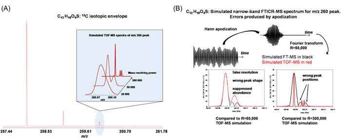
Simulation of the apodization effect on the shape of the isotopic fine structure of C12H18O4S. (A) Mass spectrum of the 13C isotopic cluster and a change in the shape of the fine structure peaks with mass resolving power at m/z 260; (B) Distortion of the fine structure peak shapes of the FTICR mass domain at m/z 260 due to apodization. The apodization function was chosen such that if there were no isotopic fine structure the resolution would be ~50,000 FWHM. Also shown, the overlays of the TOF‐MS simulations at two TOF‐MS resolutions, ~50,000 and ~300,000 FWHM. FWHM, full width at half maximum; TOF, time of flight‐mass spectrometry. [Color figure can be viewed at wileyonlinelibrary.com]
Figure 8B illustrates the processing of a narrow band ICR signal for the isotopic fine structure cluster at m/z 260, going from the time (ultimately) to the mass domain. The apodization function was chosen such that if there were no isotopic fine structure the resolution would be ~50,000 FWHM. Also shown in Figure 8B are the overlays of the TOF‐MS simulations at two TOF‐MS resolutions, ~50,000 and ~300,000 FWHM. The TOF‐MS simulations are not subject to the kind of peak distortions being discussed in this section relating to FT‐MS signal processing. Thus, the TOF‐MS simulations represent what the isotopic fine structure cluster should look like in the absence of peak distortions.
Let us first consider the comparison of the TOF‐MS simulation to the FT‐MS simulation, both at resolution of ~50,000. The striking thing about this comparison is that the FT‐MS result shows significant distortions, including suppression of the abundance (by ~18% as computed by peak area, most of which is in the higher‐mass region), a distortion of the overall shape of the isotopic fine structure profile (especially in the higher‐mass region), and perhaps most strikingly, false resolution in the higher‐mass region. We know that the resolution is false because at a resolution of ~50,000 it is impossible for the two main isotopic fine structure peaks in the high‐mass region (at masses 260.09684 and 260.09931 Da) to be resolved. This is illustrated in the TOF‐MS simulation at 50,000 resolution, which shows not even a hint of resolution of these two peaks. In fact, it would take a resolution well over 200,000 to well‐resolve these two peaks.
The comparison of the FT‐MS simulation at R=50,000 to the TOF‐MS simulation at R=300,000 reveals another disturbing error in the FT‐MS result. Although there are two peaks in the higher‐mass region of the FT‐MS simulation (attributable, as already noted, to false resolution), those two peaks are placed at the wrong masses. This is evident when compared to the TOF‐MS simulation because, even though the higher‐mass region of the TOF‐MS region is dominated by two peaks, from the figure it is clear that they are not located at the same masses as the two peaks in the FT‐MS simulation.
As a final error in the FT‐MS results we note that the centroid of the isotopic fine structure cluster is shifted to lower mass on account of the suppressed abundance in the higher‐mass region of the isotopic fine structure profile. In FT‐MS simulations done at much lower resolution(where the mass‐domain peak width is much wider than the isotopic fine structure envelope) and ultrahigh resolution (where the isotopic fine structure is well‐resolved) the distortions discussed in this section disappear (data not shown).
From these results, one might be tempted to conclude that one can avoid distortions in the isotopic distributions by operating at either low or extremely high resolution. This is often the case, but some caveats must be kept in mind. First, if there is a long delay between the excitation and detections phases of an FTICR‐MS experiment there may be time for dephasing of the signal to occur from isotopic fine structure signal components. In that case, one can expect distortions of the isotopic fine structure clusters, such as amplitude distortions. Also, if the isotopic fine structure is too rich, the signal components may fail to sufficiently re‐phase over the time scale of the experiment. In that case, the abundance of the isotopic fine structure cluster will not be recovered correctly, and the abundance will be too low. It can even get worse as the apodization function is widened.
To understand the apparent paradox that things can get worse as the apodization function is widened, consider an isotopic peak having an extremely dense isotopic fine structure, dense to the extent that it is virtually indistinguishable from a continuous function. For convenience let us assume that the isotopic fine structure has a Gaussian envelope. By implication, the frequency spectrum is also a Gaussian function, and assuming that the signal components are in phase at t = 0, the time domain signal decays according to a Gaussian envelope. With this in mind, let us consider a sinusoidal time domain signal, modified with a Gaussian envelope. We first note that it is not a contrived model but can apply to real molecules. Based on calculations to model the isotopic profiles of large biomolecules, it has been noted that as the molecular weight increases, the isotopic fine structure in the main peaks in the isotopic profiles become extremely dense and the overall envelope of a single isotopic fine structure cluster (i.e., nominal isotopic peak) approaches a Gaussian profile (Dittwald et al., 2015). This implies that in a mass spectrometer, that depends on frequency measurement, such as an FTICR‐MS or an Orbitrap MS, the envelope of the signal decay profile will approach a Gaussian function, so the time domain signal for this case is of the form:
| (5) |
where is a characteristic dephasing time for the signal from the ion packet and is the center frequency associated with the isotopic fine structure cluster. Assume that a Hann apodization function is applied:
| (6) |
where is the apodized signal and is the width of the apodization function. If necessary, the signal can be extended beyond this interval by zero filling.
If the apodization function is very wide, defined here as one can expand the Hann function as a Taylor series, keeping only the first nonzero term, resulting in
| (7) |
This relationship becomes exact in the limit of . The envelope of the apodized decay function under these conditions is therefore
| (8) |
This is a bell‐shaped function whose amplitude scales as , implying that as the apodization function width approaches infinity the calculated signal level approaches zero proportionally to .
The other notable feature of this envelope function is that, aside from amplitude scaling, its shape is the same, regardless of the value of , provided only that . This means that making the apodization wider does not widen the apodized time‐domain function. This further implies that there is a limit to the improvement in resolution that can result from using a wider apodization function. This constraint seems somewhat counterintuitive because the usual experience is that acquiring a longer signal transient (along with using a wider apodization function) produces a higher resolution spectrum. One practical implication of this is that if one is investigating very large biomolecules by Fourier transform mass spectrometric methods there is little reason to waste a laboratory's resources by trying to push the resolution beyond this fundamental limit by acquiring a longer signal transient, particularly since this can result in a catastrophic loss of signal amplitude of the isotopic peaks.
The underlying reason for this seemingly pathological behavior is that once the isotopic fine structure becomes sufficiently dense there is no hope that the signal components will come back into phase, and the time domain signal decays monotonically toward zero under any practical laboratory time scale.
One can take several lessons from these simulations. First, although rich isotopic fine structure clusters tend to be found in mid‐sized molecules or large molecules, the effects can also show up in small molecules, as illustrated in the C12H18O4S example. Second, as a rule of thumb, the various distortions tend to be most severe when the width of the apodization function is characterized by the following inequality
| (9) |
where is the width of the envelope of the isotopic fine structure cluster in the mass domain, is average the spacing between the isotopic fine structure peaks within the cluster, and is the width of the apodization function in the mass domain, keeping in mind that is inversely proportional to the width of the apodization function in the frequency domain.
Third, the distortions may affect some parts of an isotopic fine structure more than others. This was shown in the C12H18O4S example where it was primarily the high‐mass side of the fine structure cluster at m/z 260 that was distorted.
Fourth, although not directly investigated in this simulation, it can be shown that the distortions tend to be more prominent in larger molecules, such as large biomolecules, because larger molecules tend to have richer isotopic fine structure patterns, both in terms of wider isotopic fine structure envelopes and the density of fine structure peaks within the isotopic fine structure cluster.
Fifth, though not shown directly in these simulations, other experience with additional simulations shows that the distortions tend to be worse for the higher isotopes. This is because the higher isotope peaks tend to have richer isotopic fine structure patterns. In fact the monoisotopic peak has no fine structure, so it is not distorted by the mechanism discussed in this section of the paper. However, an exception occurs for certain compounds that have no isotopic fine structure, such as pure carbon clusters, in which case there will be no distortions arising from the mechanism discussed in this section of the paper.
Finally, if the isotopic fine structure cluster becomes so rich in fine structure peaks that they cannot be resolved on the practical time scale of an experiment then widening the apodization function provides no benefit: the resolution does not improve and the abundance of the isotopic peaks suffers a catastrophic decrease. This may happen for extremely large biomolecules.
A more detailed discussion can be found in the earlier works (Rockwood & Erve, 2014), which introduce the theory presented here and uses it to rationalize experimental results (Blake et al., 2011; Erve et al., 2009).
7. PEAK APEX OR PEAK AREA?
When isotopic fine structure exists the question arises “when is it appropriate to use peak apex‐based abundances to represent abundances in place of peak area‐based peak abundances?” A similar question applies to evaluation of mass. Let us state without proof at the outset that, in the absence of peak distortion effects, including those discussed in this paper, peak area is, generally speaking, an unbiased estimator of relative isotopic peak abundances, and the closely related method of quadrature (i.e., center of mass measurements using numerical integration over the peak profile) gives an unbiased estimate of mass. Peak apexes of isotopic peaks can also be used to evaluate abundance and mass under certain circumstances, but this is not always true.
We will illustrate this with a simple example, the isotopic peaks of BrCl. Including fine structure, there are four peaks with the isotopic compositions of 79Br35Cl, 79Br37Cl, 81Br35Cl, and 81Br37Cl. Listed as (mass, abundance normalized to unity for full isotopic distribution) ordered pairs this list becomes (assuming zero for electron mass): (113.88719, 0.383), (115.88424, 0.124), (115.88514, 0.372), and (117.88219, 0.121). The two peaks in the middle of this list both have 116 nucleons and are separated by only 0.0009 Da which is equivalent to ~8 ppm difference. If one lists these peaks as ordered pairs according to nucleon number and ignores the isotopic fine structure, the list can be denoted as (114, 0.383), (116, 0.496), and (118, 1.121).
What happens to the spectra as resolution increases? As can be seen in Table 4, for the 116‐nucleon peak, both the peak apex‐based abundance and peak apex‐based mass vary with the resolution, but the area‐based abundance and quadrature‐based mass do not depend on the resolution. Figure 9 represents this in visual form. Even for the 33,000 resolution case, for which there is no hint of isotopic fine structure if evaluated by visual inspection, both the abundance and the mass are shifted relative to the correct values, although the mass is only shifted by 0.4 ppm. For the 114‐ and 118‐nucleon peaks neither the abundance nor the mass vary with resolution if evaluated using peak apex. Some of these effects are shown in references (Rockwood et al., 1996; Werlen, 1994) illustrated with a different compound (Figure 10).
Table 4.
Masses and abundances of isotopic peaks of BrCl evaluated according to peak apexand area or quadrature, listed according to FWHM resolution.
| Resolution (FWHM) | Peak apex‐based abundance | Area‐based abundance | Peak apex‐based mass | Quadrature‐based mass |
|---|---|---|---|---|
| 33,000 | 0.477 | 0.496 | 115.88496 | 115.88492 |
| 83,000 | 0.409 | 0.496 | 115.88509 | 115.88492 |
| 116,000 | 0.379 | 0.496 | 115.88517 | 115.88492 |
Figure 10.

Simulation of the effect of resolution on 116 Da peak of BrCl. Peak widths are 0.0010, 0.0014, and 0.0035 Da. Simulated spectra are normalized to set the peak apexof the mono‐isotopic peak (115 Da) to a value of 1.00 at each resolution setting. [Color figure can be viewed at wileyonlinelibrary.com]
From this, it is clear that peak apex abundances can be substituted for integrated peak area abundances at low resolution, but as the instrument‐limited peak width approaches the width of the isotopic fine structure envelope one should abandon peak apex abundances and use peak areas instead. This general conclusion applies to all types of mass analyzers, as long as the analyzer and data reduction themselves to not further distort the peak abundances. However, see the discussion in Section 5 of this paper for a discussion of FTMS where certain additional considerations may apply. An exception occurs if the isotopic peaks contain no fine structure, such as in carbon clusters, for which peak apexes can be used to evaluate abundance and mass.
8. CONCLUDING REMARKS
In this manuscript, we have described the various physical, instrumental, electronic, and algorithmic phenomena that could disturb the appearance of an observed isotope pattern in a spectrum from the theoretically computed isotope distribution. In this overview, we follow a molecular analyte from sample toward signal. A first artifact is caused by deviations in the sample with respect to the IUPAC or NIST definition of the elemental isotope composition in a terrestrial matter that already can lead to a discordance in the isotope patterns. Second, stochastic principles can interfere with the appearance of the isotope distribution. It all depends on the number of ions used to sample the intrinsic isotope distribution of an analyte in a sample. A better ion statistic leads to observed isotope patterns that are more similar to these intrinsic isotopologues. An important remark here is that there is an intensity‐dependency. Lower ion counts typically result in low‐intense signals that display a larger sampling variation than with the high‐intense counterparts. Third, when compressing charged ions in small spaces, as is the case in modern trapping devices, so‐called space‐charge effects come into play that affect all aspects of high‐resolution mass spectrometry, including peaks related to poly‐isotopic elements, and the relative abundances of these peaks in the recorded fine structures. Even when the trap is not overfilled, ions that are stored in close proximity, with a similar m/z ratio for a long acquisition time will experience Coulombic interactions that are detrimental for the ion signal. This effect will cause three types of disturbances to the observed isotope distribution: (A) distortion of measured relative signal intensities of lower abundance isotopic species; (B) coalescence of ion bundles of similar m/z leading to an aggregation of fine isotope variants; and (C) systematic shift in the measured masses. Fourth, after detection of the harmonic ion signal and digitization, additional signal processing is performed, especially in the case of Fourier‐transform mass spectrometry, to transform the time‐domain transient into the frequency‐domain (i.e., mass domain). Although the Fourier transform is a linear operator, the apodization of the decaying transient signal is not. The choice of the various FT‐signal processing parameters (zero‐filing, apodization function, window width, and window location) can have various unwanted effects on the isotope distribution. This effect is particularly noticeable in the case of dephasing of the ion bundles that lead to destructive interference. When the apodization is the window is chosen in a location where this destructive interference is complete then this may cause an attenuated signal with respect to the theoretical isotope distribution. Or when the isotope‐fine structure is too rich, the signal components may fail to re‐phase and therefore go undetected. Fifth, the question of whether the peak apex can be used to determine mass and ion abundance in place of a quadrature‐based calculation to estimate the centroided mass and area under the curve is evaluated. It is shown that in some cases this can lead to errors.
Albeit, we have tried to be exhaustive as possible, there are some processes not described in this manuscript. For example, the structure of the electronic noise that superposes with the signal after acquisition. A meritorious attempt to model the noise structure of QTOF spectra is provided by Du et al. (2008). Another artifact neglected in this overview is detector saturation in linear ion traps or TOF instruments. Once signal intensities become too large in electron multipliers or particle detectors we move outside the linear range of detection and signal intensities will become flattened. This saturation has an obvious effect on the observed isotope pattern and will lead to errors in quantifying the signal. Remedial measures have been devised to correct for this quantification error postacquisition (Bilbao et al., 2018)
In the introduction, we have enlisted numerous bioinformatics applications that benefit from working on clean mass spectra with undistorted isotope patterns. However, many processes will interfere with the correct measurement of the spectra that lead to potential errors when using these bioinformatics tools. It is impossible for a mass spectrometrist or data scientist to take all these effects into consideration and quantify and account for these errors when analysing an isotope pattern in a spectrum. Finally, with this manuscript, we want to create awareness that many off‐the‐shelf bioinformatics tools come with various premises and assumptions that may or may not be compatible with your instrumental set‐up. Therefore, we recommend calibrating your bioinformatics tools on selected, well‐known yet realistic standards to better understand the impact of the default thresholds and optimize the fine‐tuning of your algorithm for your laboratory. The concept of one‐size‐fits‐all is unfortunately not applicable in the field of mass spectrometry.
Biographies
Jürgen Claesen received his M.Sc. degrees in Biochemistry (K.U. Leuven) and in Statistics (UHasselt). In 2013, he received a PhD in Statistics (UHasselt). Currently, he is an assistant professor in the Epidemiology and Data Science department of the Amsterdam University Medical Center. His research focuses on the development of statistical and computational methods for high‐dimensional data, including mass spectrometry.

Alan Rockwood received his PhD in chemistry 1981 from Utah State University with a specialization in physical chemistry. Since then he has worked in several laboratories, two of which were Battelle Pacific Northwest Laboratory, where he focused on mass spectrometry fundamentals and instrumentation design, and University of Utah/ARUP Laboratories, where he was Scientific Director for Mass Spectrometry and Professor (Clinical) of Pathology. He is currently an Emeritus Professor (Clinical) of Pathology of the University of Utah School of Medicine and was a founding Co‐Editor‐in‐Chief of Clinical Mass Spectrometry, now known as Journal of Mass Spectrometry and Advances in the Clinical Lab (JMSACL).

Mikhail Gorshkov graduated from Moscow Institute of Physics and Technology with a PhD in Physics and Mathematics in 1987. His early research was under Prof. Nikolaev's supervision in precise atomic mass measurements and related mass spectrometry instrumentation. Since then he worked at The Ohio State University and Pacific Northwest National Laboratory with the main focus on developing mass spectrometry‐based approaches for studying proteins. In 2002 he founded the Laboratory of Physical and Chemical Methods for Structure Analysis at V.L. Talrose Institute for Energy Problems of Chemical Physics, Russian Academy of Sciences, and became Director of this Institute in 2017. His current main areas of research are broadly within biological mass spectrometry and bioinformatics with applications in proteomics.

Dirk Valkenborg received his M.Sc. degree in Electrotechnical Engineering from the K.U. Leuven in 2004. He received his PhD degree in Mathematics and Statistical Bioinformatics from the University of Hasselt in 2008 and obtained an MSc degree in Biostatistics in 2009 from the same institution. Currently, he is active as a professor in bioinformatics and data sciences at the Center for Statistics at Hasselt University where he leads a team with a focus on computational methodologies for the low‐level interpretation of omics‐related data and machine learning.

Claesen J, Rockwood A, Gorshkov M, Valkenborg D. The isotope distribution: a rose with thorns. Mass Spectrom Rev. 2025;44:22–42. 10.1002/mas.21820.
All authors contributed equally and share first authorship.
REFERENCES
- Aebersold R, Mann M. 2003. Mass spectrometry‐based proteomics. Nature. 422: 198‐207. [DOI] [PubMed] [Google Scholar]
- Aizikov K, Mathur R, O'Connor PB. 2009. The spontaneous loss of coherence catastrophe in Fourier transform ion cyclotron resonance mass spectrometry. J Am Soc Mass Spectrom. 20(2): 247‐256. [DOI] [PMC free article] [PubMed] [Google Scholar]
- Allwood JW, Parker D, Beckmann M, Draper J, Goodacre R. 2011. Fourier transform ion cyclotron resonance mass spectrometry for plant metabolite profiling and metabolite identification. In: Hardy N., Hall R. (eds) Plant Metabolomics. Methods in Molecular Biology (Methods and Protocols), Vol. 860. pp 157‐176. Humana Press. [DOI] [PubMed] [Google Scholar]
- Bartelink EJ, Chesson LA. 2019. Recent applications of isotope analysis to forensic anthropology. Forensic Sci Res. 4(1): 29‐44. [DOI] [PMC free article] [PubMed] [Google Scholar]
- Beavis RC. 1993. Chemical mass of carbon in proteins. Anal Chem. 65: 496‐497. [Google Scholar]
- Bilbao A, Gibbons BC, Slysz GW, Crowell KL, Monroe ME, Ibrahim YM, Smith RD, Payne SH, Baker ES. 2018. An algorithm to correct saturated mass spectrometry ion abundances for enhance quantitation and mass accuracy in omic studies. Int J Mass Spectrom. 427: 91‐99. [DOI] [PMC free article] [PubMed] [Google Scholar]
- Bittremieux W, Valkenborg D, Martens L, Laukens K. 2017. Computational quality control tools for mass spectrometry proteomics. Proteomics. 17(3‐4): 1600159. [DOI] [PubMed] [Google Scholar]
- Blake SW, Walker SH, Muddiman DC, Hinks D., Beck, KR. 2011. Spectral accuracy and sulfur counting capabilities of the LTQ‐FT‐ICR and the LTQ‐Orbitrap XL for small molecule analysis. J Am Soc Mass Spectrom. 22: 2269–2275. [DOI] [PMC free article] [PubMed] [Google Scholar]
- Boldin IA, Nikolaev EN. 2009. Theory of peak coalescence in Fourier transform ion cyclotron resonance mass spectrometry. Rapid Commun Mass Spectrom. 23(19): 3213‐3219. [DOI] [PubMed] [Google Scholar]
- Boldin IA, Nikolaev EN. 2011. Fourier transform ion cyclotron resonance cell with dynamic harmonization of the electric field in the whole volume by shaping of the excitation and detection electrode assembly. Rapid Commun Mass Spectrom. 25(1): 122‐126. [DOI] [PubMed] [Google Scholar]
- Budzikiewicz H, Grigsby RD. 2006. Mass spectrometry and isotopes: a century of research and discussion. Mass Spectrom Rev. 25(1): 146‐157. [DOI] [PubMed] [Google Scholar]
- Caimi RJ, Brenna JT. 1996. Direct analysis of carbon isotope variability in albumins by liquid flow‐injection isotope ratio mass spectrometry. J Am Soc Mass Spectrom. 7 (6): 605–610. [DOI] [PubMed] [Google Scholar]
- Chen SP, Comisarow MB, 1991. Simple physical models for coulomb‐induced frequency shifts and coulomb‐induced inhomogeneous broadening for like and unlike ions in Fourier transform ion cyclotron resonance mass spectrometry. Rapid Commun Mass Spectrom. 5(10): 450‐455. [Google Scholar]
- Claesen J, Valkenborg D, Burzykowski T. 2020. De novo prediction of the elemental composition of peptides and proteins based on a single mass. J Mass Spectrom. 55(8): e4367. [DOI] [PubMed] [Google Scholar]
- Claesen J, Dittwald P, Burzykowski T, Valkenborg D. 2012a. An efficient method to calculate the aggregated isotopic distribution and exact center‐masses. J Am Soc Mass Spectrom. 23(4): 753‐763. [DOI] [PubMed] [Google Scholar]
- Claesen J, Dittwald P, Burzykowski T, Valkenborg D. 2012b. Reply to the comment on “an efficient method to calculate the aggregated isotopic distribution and exact center‐masses” by Claesen et al. J Am Soc Mass Spectrom. 23(10): 1828‐1829. [DOI] [PubMed] [Google Scholar]
- Claesen J, Lermyte F, Sobott F, Burzykowski T, Valkenborg D. 2015. Differences in the elemental isotope definition may lead to errors in modern mass‐spectrometry‐based proteomics. Anal Chem. 87(21): 10747‐10754. [DOI] [PubMed] [Google Scholar]
- Cody RB, Tamura J, Musselman BD. 1992. Electrospray ionization/magnetic sector mass spectrometry: calibration, resolution, and accurate mass measurements. Anal Chem. 64: 1561‐1570. [Google Scholar]
- Comisarow MB, Marshall AG. 1974. Fourier transform ion cyclotron resonance spectroscopy. Chem Phys Lett. 25(2): 282‐283. [Google Scholar]
- Coplen TB, Holden NE. 2011. Atomic weights—no longer constants of nature. Chem Int. 33 (2): 10‐15. [Google Scholar]
- Cox J, Neuhauser N, Michalski A, Scheltema RA, Olsen JV, Mann M. 2011. Andromeda: a peptide search engine integrated into the MaxQuant environment. J Proteome Res. 10(4): 1794‐805 [DOI] [PubMed] [Google Scholar]
- De Vijlder T, Valkenborg D, Lemière F, Romijn EP, Laukens K, Cuyckens F. 2018. A tutorial in small molecule identification via electrospray ionization‐mass spectrometry: the practical art of structural elucidation. Mass Spectrom Rev. 37(5): 607‐629. [DOI] [PMC free article] [PubMed] [Google Scholar]
- DeNiro MJ, Epstein S. 1978. Influence of diet on the distribution of carbon isotopes in animals. Geochim Cosmochim Acta. 42: 495‐506. [Google Scholar]
- Dittwald P, Valkenborg D, Claesen J, Rockwood AL, Gambin A. 2015. On the fine isotopic distribution and limits to resolution in mass spectrometry, J Am Soc Mass Spectrom. 26(10): 1732‐1745. [DOI] [PMC free article] [PubMed] [Google Scholar]
- Du P, Stolovitzky G, Horvatovich P, Bischoff R, Lim J, Suits F. 2008. A noise model for mass spectrometry based proteomics. Bioinformatics . 24(8): 1070‐1077. [DOI] [PubMed] [Google Scholar]
- Erve JCL, Gu, M , Wang Y, DeMaio W, Talaat RE. 2009. Spectral accuracy of molecular ions in an LTQ/Orbitrap mass spectrometer and implications for elemental composition determination. J Am Soc Mass Spectrom. 20: 2058–2069. [DOI] [PubMed] [Google Scholar]
- Goldfarb D, Lafferty MJ, Herring LE, Wang W, Major MB. 2018. Approximating isotope distributions of biomolecule fragments. ACS Omega. 3(9): 11383‐11391. [DOI] [PMC free article] [PubMed] [Google Scholar]
- Gordon EF, Muddiman DC. 2001. Impact of ion cloud densities on the measurement of relative ion abundances in Fourier transform ion cyclotron resonance mass spectrometry: experimental observations of coulombically induced cyclotron radius perturbations and ion cloud dephasing rates. J Mass Spectrom. 36(2): 195‐203. [DOI] [PubMed] [Google Scholar]
- Gorshkov MV, Marshall AG, Nikolaev EN. 1993. Analysis and elimination of systematic errors originating from coulomb mutual interaction and image charge in Fourier transform ion cyclotron resonance precise mass difference measurements. J Am Soc Mass Spectrom. 4(11): 855‐868. [DOI] [PubMed] [Google Scholar]
- Gorshkov MV, Fornelli L, Tsybin YO. 2012. Observation of ion coalescence in Orbitrap Fourier transform mass spectrometry. Rapid Commun Mass Spectrom. 26(15), 1711‐1717. [DOI] [PubMed] [Google Scholar]
- Gorshkov MV, Good DM, Lyutvinskiy Y, Yang H, Zubarev RA. 2010. Calibration function for the Orbitrap FTMS accounting for the space charge effect. J Am Soc Mass Spectrom. 21(11): 1846‐1851. [DOI] [PubMed] [Google Scholar]
- He F, Hendrickson CL, Marshall AG. 2001. Baseline mass resolution of peptide isobars: A record for molecular mass resolution. Anal Chem. 73(3): 647‐650. [DOI] [PubMed] [Google Scholar]
- Hendrickson CL, Quinn JP, Kaiser NK, Smith DF, Blakney GT, Chen T, Marshall AG. Weisbrod CR, Beu SC. 2015. 21 Tesla Fourier transform ion cyclotron resonance mass spectrometer: a national resource for ultrahigh resolution mass analysis. J Am Soc Mass Spectrom. 26(9): 1626‐32. [DOI] [PubMed] [Google Scholar]
- Horn D., Zubarev R., McLafferty F. 2000. Automated reduction and interpretation of high resolution electrospray mass spectra of large molecules. J Am Soc Mass Spectrom. 11: 320‐332. [DOI] [PubMed] [Google Scholar]
- Huang J, Tiedemann PW, Land DP, McIver RT, Hemminger JC. 1994. Dynamics of ion coupling in an FTMS ion trap and resulting effects on mass spectra, including isotope ratios. Int J Mass Spectrom Ion Proc. 134(1): 11‐21. [Google Scholar]
- Jeffries JB, Barlow SE, Dunn GH. 1983. Theory of space‐charge shift of ion cyclotron resonance frequencies. Int J Mass Spectrom Ion Proc. 54(1‐2): 169‐187. [Google Scholar]
- Kaiser NK, Bruce JE. 2005. Observation of increased ion cyclotron resonance signal duration through electric field perturbations. Anal Chem. 77(18): 5973‐5981. [DOI] [PubMed] [Google Scholar]
- Kaur P, O'Connor PB. 2004. Use of statistical methods for estimation of total number of charges in a mass spectrometry experiment. Anal Chem. 76: 2756‐2762. [DOI] [PubMed] [Google Scholar]
- Kaur P, O'Connor PB. 2007. Quantitative determination of isotope ratios from experimental isotopic distributions. Anal Chem. 79: 1198‐1204. [DOI] [PMC free article] [PubMed] [Google Scholar]
- Kendall C, Caldwell EA. 1998. Fundamentals of isotope geochemistry in isotope tracers. In Kendall C. and McDonnell J. J. Catchment Hydrology, Amsterdam: Elsevier. 51‐86. [Google Scholar]
- Kharchenko A, Vladimirov G, Heeren RM, Nikolaev EN. 2012. Performance of Orbitrap mass analyzer at various space charge and non‐ideal field conditions: simulation approach. J Am Soc Mass Spectrom. 23(5): 977‐987. [DOI] [PubMed] [Google Scholar]
- Kim S, Rodgers RP, Marshall AG. 2006. Truly “exact” mass: elemental composition can be determined uniquely from molecular mass measurement at ∼0.1 mDa accuracy for molecules up to ∼500 Da, Int. J. Mass Spectrom. 251(2‐3): 260‐265. [Google Scholar]
- Kind T, Fiehn O. 2006. Metabolomics database annotations via query of elemental compositions: mass accuracy is insufficient even at less than 1 ppm. BMC Bioinform. 7: 234. [DOI] [PMC free article] [PubMed] [Google Scholar]
- Kind T, Fiehn O. 2007. Seven Golden Rules for heuristic filtering of molecular formulas obtained by accurate mass spectrometry. BMC Bioinform. 8:105. [DOI] [PMC free article] [PubMed] [Google Scholar]
- Koehler, G. , Kardynal, KJ , Hobson, KA. 2019. Geographical assignment of polar bears using multi‐element isoscapes. Sci Rep. 9: 9390. [DOI] [PMC free article] [PubMed] [Google Scholar]
- Kubinyi H. 1991. Calculation of isotope distributions in mass spectrometry. A trivial solution for a non‐trivial problem. Anal Chim Acta. 247(1), 107‐119. [Google Scholar]
- Łącki MK, Valkenborg D, Startek M. 2020. IsoSpec2: ultrafast fine structure calculator. Anal Chem. 92, 14, 9472–9475. [DOI] [PubMed] [Google Scholar]
- Łącki MK, Startek M, Valkenborg D, Gambin A. 2017. IsoSpec: hyperfast fine structure calculator. Anal Chem. 89(6): 3272‐3277. [DOI] [PubMed] [Google Scholar]
- Ledford EB Jr., Rempel DL, Gross ML. 1984. Space charge effects in Fourier transform mass spectrometry. Mass calibration. Anal Chem. 56(14): 2744‐2748. [DOI] [PubMed] [Google Scholar]
- Li H, Wolff JJ, Van Orden SL, Loo JA. 2014. Native top‐down electrospray ionization‐mass spectrometry of 158kDa protein complex by high‐resolution Fourier transform ion cyclotron resonance mass spectrometry. Anal Chem. 86(1): 317‐20. [DOI] [PMC free article] [PubMed] [Google Scholar]
- Lozano DCP, Gavard R, Arenas‐Diaz JP, Thomas MJ, Stranz DD, Mejía‐Ospino E, Guzman A, Spencer SEF, Rossell D, Barrow MP. 2019. Pushing the analytical limits: new insights into complex mixtures using mass spectra segments of constant ultrahigh resolving power. Chem Sci. 10, 6966‐6978. [DOI] [PMC free article] [PubMed] [Google Scholar]
- MacCoss MJ, Toth MJ, Matthews DE. 2001. Evaluation and optimization of ion‐current ratio measurements by selected‐ion‐monitoring mass spectrometry. Anal Chem. 73: 2976‐2984. [DOI] [PubMed] [Google Scholar]
- Makarov A. 2000. Electrostatic axially harmonic orbital trapping: a high‐performance technique of mass analysis. Anal Chem. 72(6): 1156‐1162. [DOI] [PubMed] [Google Scholar]
- Makarov A., Denisov E. 2009. Dynamics of ions of intact proteins in the Orbitrap mass analyzer. J Am Soc Mass Spectrom. 20(8): 1486‐1495. [DOI] [PubMed] [Google Scholar]
- Mann M, Meng CK, Fenn JB. 1989. Interpreting mass spectra of multiply charged ions. Anal Chem. 61(15): 1702–1708. [Google Scholar]
- Marshall AG, Hendrickson CL, Jackson GS. 1998. Fourier transform ion cyclotron resonance mass spectrometry: a primer. Mass Spectrom Rev. 17(1): 1‐35. [DOI] [PubMed] [Google Scholar]
- Masselon C, Tolmachev AV, Anderson GA, Harkewicz R, Smith RD. 2002. Mass measurement errors caused by “local” frequency perturbations in FTICR mass spectrometry. J Am Soc Mass Spectrom. 13(1): 99‐106. [DOI] [PubMed] [Google Scholar]
- McKinney CR, McRea IM, Epstein S, Allen HA, Urey HC. 1950. Improvements in mass spectrometers for measurement of small differences in isotope abundance ratios. Rev Sci Instrum. 21:724‐730. [DOI] [PubMed] [Google Scholar]
- Miladinović SM, Kozhinov AN, Gorshkov MV, Tsybin YO. 2012. On the utility of isotopic fine structure mass spectrometry in protein identification. Anal Chem. 84(9): 4042–4051. [DOI] [PubMed] [Google Scholar]
- Mitchell DW, Smith RD. 1995. Cyclotron motion of two coulombically interacting ion clouds with implications to Fourier‐transform ion cyclotron resonance mass spectrometry. Phys Rev E. 52(4): 4366‐4386. [DOI] [PubMed] [Google Scholar]
- Miura В, Tsuji Y, Takahashi K., Wariishi H, Saito K. 2010. A strategy for the determination of the elemental composition by Fourier transform ion cyclotron resonance mass spectrometry based on isotopic peak ratios. Anal Chem. 82(13): 5887‐5891. [DOI] [PubMed] [Google Scholar]
- Nagao T, Yukihira D, Fujimura Y, Saito K, Takahashi K, Miura D, Wariishi H. 2014. Power of isotopic fine structure for unambiguous determination of metabolite elemental compositions: In silico evaluation and metabolomic application. Analytica Chim Acta. 813: 70‐76. [DOI] [PubMed] [Google Scholar]
- Nagornov KO, Gorshkov MV, Kozhinov AN, Tsybin YO. 2014. High‐resolution Fourier transform ion cyclotron resonance mass spectrometry with increased throughput for biomolecular analysis. Anal Chem. 86(18): 9020‐9028. [DOI] [PubMed] [Google Scholar]
- Naito Y, Inoue M. 1994. Peak confluence phenomenon in Fourier transform ion cyclotron resonance mass spectrometry. J Mass Spectrom Soc Jpn. 42(1): 1‐9. [Google Scholar]
- Nakata MT, Hart GW, Peterson BG. 2010. Peak coalescence, spontaneous loss of coherence, and quantification of the relative abundances of two species in the plasma regime: particle‐in‐cell modeling of Fourier transform ion cyclotron resonance mass spectrometry. J Am Soc Mass Spectrom. 21(10): 1712‐1719. [DOI] [PubMed] [Google Scholar]
- Nikolaev EN, Neronov YI, Gorshkov MV, Talroze VL. 1984. Ion cyclotron resonance measurements of the mass difference between tritium and helium‐3. JETP Lett. 39(9): 534‐536. [Google Scholar]
- Nikolaev EN, Gorshkov MV, Mordehai AV, Talrose VL. 1985. Ion‐cyclotron‐resonance‐mass‐spectrometer. USSR Inventor's Certificate SU1307492.
- Nikolaev EN, Gorshkov MV, Mordehai AV, Talrose VL. 1990. Ion cyclotron resonance signal‐detection at multiples of the cyclotron frequency. Rapid Commun Mass Spectrom. 4(5): 144‐146. [Google Scholar]
- Nikolaev EN, Boldin IA, Jertz R, Baykut G. 2011. Initial experimental characterization of a new ultra‐high resolution FTICR cell with dynamic harmonization. J Am Soc Mass Spectrom. 22(7): 1125‐1133. [DOI] [PubMed] [Google Scholar]
- Nikolaev EN, Jertz R, Grigoryev A, Baykut G. 2012. Fine structure in isotopic peak distributions measured using a dynamically harmonized Fourier transform ion cyclotron resonance cell at 7 T. Anal Chem. 84(5): 2275‐2283. [DOI] [PubMed] [Google Scholar]
- Niu M, Mao X, Ying W, Qin W, Zhang Y, Qian X. 2012. Determination of monoisotopic masses of chimera spectra from high‐resolution mass spectrometric data by use of isotopic peak intensity ratio modeling. Rapid Commun Mass Spectrom. 26(16): 1875‐1886. [DOI] [PubMed] [Google Scholar]
- O'Connor PB, Little DP, McLafferty FW. 1996. Isotopic assignment in large‐molecule mass spectra by fragmentation of a selected isotopic peak. Anal Chem. 68, 3, 542–545. [DOI] [PubMed] [Google Scholar]
- Pan Y, Ridge DP, Rockwood AL. 1988. Harmonic signal enhancement in ion cyclotron resonance mass spectrometry using multiple electrode detection. Int J Mass Spectrom Ion Proc. 84 (3): 293‐304. [Google Scholar]
- Pan Y, Ridge DP, Wronka J, Rockwood AL. 1987. Resolution improvement by using harmonic detection in an ion cyclotron resonance mass spectrometer. Rapid Commun Mass Spectrom. 1(7‐8): 120‐121. [Google Scholar]
- Peurrung AJ, Kouzes RT. 1994. Long‐term coherence of the cyclotron mode in a trapped ion cloud. Phys Rev E. 49(5): 4362‐4368. [DOI] [PubMed] [Google Scholar]
- Peurrung AJ, Kouzes RT. 1995. Analysis of space‐charge effects in cyclotron resonance mass spectrometry as coupled gyrator phenomena. Int J Mass Spectrom Ion Proc. 145(3): 139‐153. [Google Scholar]
- Peurrung AJ, Kouzes RT, Barlow SE. 1996. The non‐neutral plasma: an introduction to physics with relevance to cyclotron resonance mass spectrometry. Int J Mass Spectrom Ion Proc. 157‐158: 39‐83. [Google Scholar]
- Popov IA, Nagornov K, Vladimirov GN, Kostyukevich YI, Nikolaev EN. 2014. Twelve million resolving power on 4.7 T Fourier transform ion cyclotron resonance instrument with dynamically harmonized cell—observation of fine structure in peptide mass spectra. J Am Soc Mass Spectrom. 25(5): 790‐799. [DOI] [PubMed] [Google Scholar]
- Renard BY, Kirchner M, Steen H, Steen JA, Hamprecht FA. 2008. NITPICK: peak identification for mass spectrometry data. BMC Bioinform. 9: 355. [DOI] [PMC free article] [PubMed] [Google Scholar]
- Rockwood AL, Erve JC. 2014. Mass spectral peak distortion due to Fourier transform signal processing. J Am Soc Mass Spectrom. 25(12): 2163‐2176. [DOI] [PubMed] [Google Scholar]
- Rockwood AL, Kushnir MM, Nelsen GJ. 2003. Dissociation of individual isotopic peaks: predicting isotopic distributions of product ions in MSN. J Am Soc Mass Spectrom. 14: 311–322. [DOI] [PubMed] [Google Scholar]
- Rockwood AL, Palmblad M. 2013. Isotopic distributions. In Matthiesen R (ed). Mass Spectrometry Data Analysis in Proteomics. Methods in Molecular Biology, Vol. 1007, Springer; pp. 65‐99. [DOI] [PubMed] [Google Scholar]
- Rockwood AL, Van Orden SL, Smith RD. 1995. Rapid calculation of isotope distributions. Anal Chem. 67(15): 2699–2704. [DOI] [PubMed] [Google Scholar]
- Rockwood AL, Van Orden SL, Smith RD. 1996. Ultrahigh resolution isotope distribution calculations. Rapid Commun Mass Spectrom. 10: 54‐59. [Google Scholar]
- Roussis SG, Proulx R. 2003. Reduction of chemical formulas from the isotopic peak distributions of high‐resolution mass spectra. Anal Chem. 75(6): 1470‐1482. [DOI] [PubMed] [Google Scholar]
- Schweikhard L, Lindinger M, Kluge HJ. 1990. Quadrupole‐detection FT‐ICR mass spectrometry. Int J Mass Spectrom Ion Proc. 98(1): 25‐33. [Google Scholar]
- Senko MW, Beu SC, McLafferty FW. 1995. Determination of mono‐isotopic masses and ion populations for large biomolecules from resolved isotopic distributions. J Am Soc Mass Spectrom. 6: 229‐233. [DOI] [PubMed] [Google Scholar]
- Shaw JB, Gorshkov MV, Wu Q, Paša‐Tolić L. 2018. High speed intact protein characterization using 4x frequency multiplication, ion trap harmonization, and 21 Tesla FTICR‐MS. Anal Chem. 90(9): 5557‐5562. [DOI] [PubMed] [Google Scholar]
- Shaw JB, Lin TY, Leach FE 3rd, Tolmachev AV, Tolić N, Robinson EW, Koppenaal DW, Paša‐Tolić L. 2016. 21 Tesla Fourier transform ion cyclotron resonance mass spectrometer greatly expands mass spectrometry toolbox. J Am Soc Mass Spectrom. 27(12): 1929‐1936. [DOI] [PubMed] [Google Scholar]
- Shi SDH, Hendrickson C, Marshall AG. 1998. Counting individual sulfur atoms in a protein by ultra‐highresolution Fourier transform ion cyclotron resonance mass spectrometry: Experimental resolution of isotopic fine structure in proteins. Proc Nat Acad Sci USA. 95(20): 11532–11537. [DOI] [PMC free article] [PubMed] [Google Scholar]
- Shipley ON, Matich P. 2020. Studying animal niches using bulk stable isotope ratios: an updated synthesis. Oecologia. 193: 27–51. [DOI] [PubMed] [Google Scholar]
- Stoll N, Schmidt E, Thurow K. 2006. Isotope pattern evaluation for the reduction of elemental compositions assigned to high‐resolution mass spectral data from electrospray ionization Fourier transform ion cyclotron resonance mass spectrometry. J Am Soc Mass Spectrom. 17(12): 1692‐1699. [DOI] [PubMed] [Google Scholar]
- Tai AP, Liang A, Hamey JJ, Hart‐Smith G, Wilkins MR. 2019. MS2‐deisotoper: a tool for deisotoping high‐resolution MS/MS spectra in normal and heavy isotope‐labelled samples. Proteomics 19(17): e1800444. [DOI] [PubMed] [Google Scholar]
- Tarasova IA, Surin AK, Fornelli L, Pridatchenko ML, Suvorina MY, Gorshkov MV. 2015. Ion coalescence in Fourier transform mass spectrometry: should we worry about this in shotgun proteomics? Eur J Mass Spectrom. 21(3): 459‐470. [DOI] [PubMed] [Google Scholar]
- Uechi GT, Dunbar RC. 1992. Space charge effects on relative peak heights in Fourier transform‐ion cyclotron resonance spectra. J Am Soc Mass Spectrom. 3(7): 734‐741. [DOI] [PubMed] [Google Scholar]
- Valeja SG, Kaiser NK, Xian F, Hendrickson CL, Rouse JC, Marshall AG. 2011. Unit mass baseline resolution for an intact 148kDa therapeutic monoclonal antibody by Fourier transform ion cyclotron resonance mass spectrometry. Anal Chem. 83(22): 8391‐8395. [DOI] [PMC free article] [PubMed] [Google Scholar]
- Valkenborg D, Burzykowski T. 2011. A Markov‐Chain model for the analysis of high‐resolution enzymatically 18O‐labeled mass spectra. Stat Appl Genetics Mol Biol. 10(1). [DOI] [PubMed] [Google Scholar]
- Valkenborg D, Jansen I, Burzykowski T. 2008. A model‐based method for the prediction of the isotopic distribution of peptides. J Am Soc Mass Spectrom. 19(5): 703‐712. [DOI] [PubMed] [Google Scholar]
- Valkenborg D, Mertens I, Lemière F, Witters E, Burzykowski T. 2011. The isotopic distribution conundrum. Mass Spectrom Rev. 31: 96‐109. [DOI] [PubMed] [Google Scholar]
- Wada Y, Tamura J, Musselman BD. 1992. Electrospray ionization mass spectra of hemoglobin and transferrin by a magnetic sector mass spectrometer. Comparison with theoretical isotopic distributions. Rapid Commun Mass Spectrom. 6: 9‐13. [DOI] [PubMed] [Google Scholar]
- Wang Y, Gu M. 2010. The concept of spectral accuracy for MS. Anal Chem. 82(17): 7055‐7062. [DOI] [PubMed] [Google Scholar]
- Watkinson CL, Gasson P, Rees GO, Boner, M. 2020. The development and use of isoscapes to determine the geographical origin of Quercus spp. in the United States. Forests. 11: 862. [Google Scholar]
- Weber RJM, Southam AD, Sommer U, Viant MR. 2011. Characterization of isotopic abundance measurements in high resolution FT‐ICR and Orbitrap mass spectra for improved confidence of metabolite identification. Anal Chem. 83(10): 3737‐3743. [DOI] [PubMed] [Google Scholar]
- Werlen RC. 1994. Effect of resolution on the shape of mass spectra of proteins: some theoretical considerations. Rapid Commun Mass Spectrom. 8: 976‐980. [Google Scholar]
- Werner T, Sweetman G, Savitski MF, Mathieson T, Bantscheff M, Savitski MM. 2014. Ion coalescence of neutron encoded TMT 10‐plex reporter ions. Anal Chem. 86(7): 3594‐3601. [DOI] [PubMed] [Google Scholar]
- West JB, Bowen GJ Cerling TE, Ehleringer JR. 2006. Stable isotopes as one of nature's ecological recorders. Trends Ecol Evol. 12: 408‐414. [DOI] [PubMed] [Google Scholar]
- West JB, Bowen GJ, Dawson TE, Tu KP. 2010. Isoscapes—understanding movement, pattern, and process on Earth through isotope mapping. New York, Springer. [Google Scholar]
- Wong RL, Amster IJ. 2007. Experimental evidence for space‐charge effects between ions of the same mass‐to‐charge in Fourier‐transform ion cyclotron resonance mass spectrometry. Int J Mass Spectrom. 265(2‐3): 99‐105. [DOI] [PMC free article] [PubMed] [Google Scholar]
- Yergey JA. 1983. A general approach to calculating isotopic distributions for mass spectrometry. Int J Mass Spectrom Ion Phys. 52: 13. [DOI] [PubMed] [Google Scholar]
- Zhang Z, Marshal AG. 1998. A universal algorithm for fast and automated charge state deconvolution of electrospray mass‐to‐charge ratio spectra. J Am Soc Mass Spectrom. 9(3): 225‐33. [DOI] [PubMed] [Google Scholar]
- Zubarev RA, Håkansson P, Sundqvist B. 1996. Accuracy requirements for peptide characterization by monoisotopic molecular mass measurements. Anal Chem. 68: 4060‐4063. [Google Scholar]
- Zubarev RA, Demirev PA, Håkansson P, Sundqvist B. 1995. Approaches and limits for accurate mass characterization of large biomolecules. Anal Chem. 67 (20): 3793–3798. [Google Scholar]