Single-molecule studies of repressor–DNA interactions show long-range interactions

Abstract

We have performed single-molecule studies of GFP–LacI repressor proteins bound to bacteriophage λ DNA containing a 256 tandem lac operator insertion confined in nanochannels. An integrated photon molecular counting method was developed to determine the number of proteins bound to DNA. By using this method, we determined the saturated mean occupancy of the 256 tandem lac operators to be 13, which constitutes only 2.5% of the available sites. This low occupancy level suggests that the repressors influence each other even when they are widely separated, at distances on the order of 200 nm, or several DNA persistence lengths.

One of the great challenges in protein–DNA interaction studies is to obtain information from single protein–DNA molecules, rather than ensembles of millions of molecules. To understand protein–DNA interactions at the single-molecule level, single protein molecules must be imaged with high resolution to resolve two key fundamental issues: the number of bound proteins and their locations, which requires that the DNA be extended in a linear manner. We have developed an integrated photon molecular counting (IPMC) method to determine the number of proteins bound to DNA and a platform incorporating nanofluidic channels and total internal reflection fluorescence (TIRF) microscopy to determine the location of the lactose repressor protein (LacI) bound to DNA carrying multiple tandem lac operator (lacO) insertions.

Since its use by Jacob and Monod (1) in Escherichia coli as the fundamental model for gene regulation, the LacI repressor has been one of the most intensively studied proteins in molecular biology (2–4). LacI normally exists as a tetramer consisting of two tightly coupled dimers with a dimer–dimer dissociation constant K_d of ≈10^–13 M (5). Because, in principle, tetramers can bind to two remote sites and, thus, form protein–DNA complexes, in this experiment we worked with LacI monomers to avoid aggregation problems. LacI monomers bind strongly to lacO sequences (K_d ≈ 10^–10 M; ref. 6), and the expected off rate k_off is on the order of hours (6). This slow rate allows us ample time for observation of the repressor–DNA complexes. We used a λ DNA construct containing 256 contiguous copies of the lacO target sequence (7, 8) (Fig. 1a). Each binding unit consists of a palindromic 21-bp lacO binding site, followed by a 15-bp nonspecific sequence. Because of this 15-bp spacer, we might expect that at the 60 nM monomer protein concentration used in our experiments, all 256 sites would be occupied by two GFP–LacI monomers (Fig. 1b), and we might expect no steric interaction between the contiguously bound GFP–LacI molecules. As described below, this is not the case (Fig. 1c).

Fig. 1.

GFP–LacI bound to DNA. (a) Schematic representation of the λ DNA construct with 256 tandem copies of the lacO binding units. LacO₂₅₆–DNA is 42.06 kbp long, and the 9.22-kbp lacO₂₅₆ insertion starts at 24.02 kbp. (b) Scaled model of the specific lacO sites with the 5′-AATTGTGAGCGGATAACAATT-3′ sequence, the spacer sequences between them, and the GFP–LacI proteins bound to full occupancy. The dimensions of the LacI and GFP molecules are 3 × 6 nm (2) and 3 × 4 nm (9), respectively. (c) Actual observed occupancy level. Only 2.5% of the available sites were bound.

The key idea of the IPMC method is that a fluorescent molecule will emit a mean number of photons N₀ before it irreversibly bleaches. If the emitted number of photons N_t from an illuminated region is integrated until the region is bleached, the total number of molecules that were in that region is given by n = N_t/N₀. Although this idea is simple in principle, a number of factors must be considered in practice. (i) The Poisson statistics of the photon histogram must be analyzed carefully; (ii) self-quenching by means of Förster energy transfer between the fluorescent molecules must be assessed because the fluorescent molecules in our case can be within nanometers of each other; and (iii) energy transfer between GFP–LacI and the dye (BOBO-3, dimeric cyanine nucleic acid stains) that was used to label the DNA might complicate the analysis. We have investigated these three factors for our LacI–DNA interaction study and determined that the IPMC method can be used to count molecules labeled with GFP and BOBO-3 in close proximity.

Materials and Methods

The GFP13 (S65T): lacI-I12 fusion is described in ref. 10. This fusion lacks the last 11 aa at the extreme C terminus required for tetrameriztion (7, 10, 11). The lacI-I12 mutant also has the amino acid Pro-3 replaced by Tyr-3 to increase its affinity (6, 12). Because, in our experiment, the GFP–LacI monomer concentration ranges 5–60 nM, below the dimer–monomer LacI dissociation constant K_d = 7.7 × 10^–8 M (11), we expect to observe mainly GFP–LacI monomers. Indeed, we observed ≈15% dimers at nanomolar concentrations, consistent with reported K_d values. Because each symmetric lacO site can accommodate one LacI dimer, we expect two GFP–LacI monomers to bind to one lacO sequence. The GFP–LacI fusion construct was amplified from pAFS144 (10) and cloned into the pPROTet.E protein expression vector (Clontech). The resulting GFP–LacI expression plasmid was transformed into DH5α pro cells. The cells were grown at 37°C in Luria broth medium supplemented with 34 μg/ml chloramphenicol and 50 μg/ml spectinomycin until the culture reached an optical density of 0.5 at 600 nm. Expression of GFP–LacI fusion protein was induced by growing the culture overnight in anhydrotetracycline at 100 ng/ml at 30°C. The GFP–LacI fusion was purified by using Talon metal-affinity resins (Clontech) and further characterized by a standard gel-shift assay using the end-labeled lacO sequence shown in Fig. 1.

DNA constructs with 256 tandem copies of lacO (lacO₂₅₆) were first liberated from plasmid pAFS59 (7, 8) by BamHI digestion and then ligated into the BamHI site of λ Dash II (Stratagene). The construct size was verified further by restriction analysis, and there was a clear 9-kbp band for the lacO₂₅₆ insertion, and 24- and 9-kbp bands for the two DNA tails. The broadening of the lacO₂₅₆ band indicated that ≈10–15% of the sample contained <256 copies. This construct is 42.06 kbp with a contour length L_c ≈ 14.3 μm.

Sample Preparation. The following three different samples were prepared for imaging. (i) GFP–LacI monomers and dimers were used for calibrating the IPMC technique. The proteins were diluted to 10 nM in 0.5 × Tris/borate/EDTA (TBE) and 100 μg/ml BSA. (ii) GFP–cICys-88 covalent dimer for verifying the fluorescence characteristics of GFP dimers. This sample was prepared in the same manner as the GFP–LacI sample. (iii) LacI–lacO₂₅₆ complexes. GFP–LacI monomers were first diluted to 60 nM in 0.5× TBE buffer and 100 μg/ml BSA and then incubated with 0.4 μg/ml lacO₂₅₆–DNA for 1 h in the dark at room temperature. The ratio of LacI monomer to lacO binding site was 6:1. After binding, the LacI-DNA molecules were diluted in half by adding BOBO-3 (Molecular Probes) at a dye-to-DNA ratio of one dye molecule per 5 bp. Three additional solutions were also prepared. (iv) An oxygen scavenging solution was prepared for preventing BOBO-3 bleaching (13). The reagents and their concentrations in 0.5× TBE were glucose (8 mg/ml β-d-glucose; G7528, Sigma), glucose oxidase (0.2 mg/ml; G-7016, Sigma), catalase (40 μg/ml; C-40 Sigma), and 200 mM β-mercaptoethanol. (v) A surface passivation solution of 0.5× TBE/100 μg/ml BSA/0.1% (wt/vol) performance-optimized linear polyacrylamide (POP-6, Applied Biosystems). (vi) A mixture of surface passivation and oxygen scavenging solutions was prepared by combining solution iv with 200 μg/ml BSA and 0.2% POP-6.

For imaging using a fused-silica chip, 2.5 μl of the sample and 2.5 μl of the oxygen scavenging solution were sandwiched between the fused-silica chip and a coverslip, which was then sealed with nail polish, to yield final concentrations of GFP–LacI monomers in solution i and GFP–cICys-88 dimers in solution ii of 5 nM and the concentration of GFP–LacI monomers in sample iii of 15 nM. GFP–LacI in the absence of oxygen scavenging has also been characterized, in this case, 2.5 μlof0.5× TBE was used in place of solution iv.

For samples i and ii, isolated protein stuck to the fused-silica surface after deposition. For samples iii, both unbound and bound proteins stuck to the fused-silica surface. DNA attached to the bound proteins fluctuated around them by Brownian motion. We imaged proteins stuck to the fused-silica surface with a TIRF illumination area of 50 × 40 μm.

Nanochannel Fabrication and Electrophoresis Methods. To determine the location of GFP–LacI bound to DNA, we used nanofluidic channels to elongate the DNA. The device is shown schematically in Fig. 2a. The idea was to drive DNA molecules into the microchannel and then into the nanochannels by using electrophoresis. The 1-μm-deep microchannels were fabricated by photolithography and reactive ion etching. The nanochannels were fabricated by focused ion beam milling into fused silica. Fig. 2b is a scanning electron microscopy image of a 120 × 150-nm nanochannel. Holes were sand-blasted at the end of the microchannels (disk regions) for loading the DNA. The device was then sealed with a thin fused-silica coverslip (170 μm thick) by fused-silica–fused-silica bonding (14). Reservoirs were affixed over the holes at the four ends of the microchannels, and a prism was placed on top for TIRF microscopy. The incident angle of the laser beam was 71° with respect to the vertical.

Fig. 2.

The nanofluidic device. (a) Schematic representations of the microfluidic and nanofluidic device. Blue regions are microchannels, and the bridging black lines are nanochannels where the DNA molecules (red) are elongated. DNA molecules are guided consecutively into microchannels and nanochannels by electrophoresis. (b) SEM images of a 120 × 150 nm (width × height) channel. Inset is a top view of the nanochannel showing its dimensions. (Scale bar for Inset, 100 nm.)

We passivated the channel surfaces with antisticking reagents before injecting the LacI–DNA solution. The channels were wetted by capillary force with solution v. Together, BSA and POP-6 prevent the sticking of proteins to fused-silica surfaces, whereas POP-6 reduces electroosmosis. A few hours of soaking was sufficient for the surface treatment. The surface treatment solution was then removed from the reservoirs and replaced with a mixture of equal parts solution iii and vi.

To drive DNA into the microchannels, a voltage drop was applied across the microchannel (between V₁ and V₂). After a sufficient amount of DNA appeared in the microchannel, a different voltage drop was applied across the nanochannels (between V₁ and V₄) and across the microchannel (between V₁ and V₂) simultaneously. Once a DNA molecule had entered a nanochannel, the voltage was turned off and the molecule came to rest. We then imaged the DNA at 568 nm (BOBO-3) and bound GFP–LacI protein at 488 nm using TIRF microscopy. In comparison with TIRF imaging at an open fused-silica–water interface, the nanochannels fused-silica–water interface was restricted to only 100 nm in width and depth; this 100-nm depth is less than the evanescent wave penetration of 200 nm at our excitation angle of 71°, and hence, GFP–LacI molecule TIRF imaging was unaffected in the nanochannels.

Imaging. The emitted photons from BOBO-3 (excitation/emission, 568:602 nm) and GFP (excitation/emission, 488:511 nm) were collected by using a 100× TIRF oil-immersion objective (numerical aperture, 1.45). The emitted photons went through a custom-designed dichroic mirror and an emission filter and were recorded by a charge-coupled device (CCD) camera with an intensifier (I-PentaMAX:HQ Gen III, Princeton Instruments, Trenton, NJ). The emission filters were designed to eliminate overlap between the GFP and BOBO-3 signals.

To determine the number of photons emitted by a single GFP–LacI molecule, the fluorescence counts per pixel that were received and read by the camera were converted into number of emitted photons. The total fluorescence count of a protein dot, which is typically a few pixels across and includes counts from both the protein and background, was first obtained. Then the background fluorescence count measured from nonfluorescent pixels adjacent to the dot was subtracted. Protein fluorescence counts were then converted into emitted photons by using the photoelectron-to-digital unit-conversion factor of 16.72 count/e^– (manufacturer's specification) and the collection efficiency of our microscope/camera system of 6.4%.

The following two settings were used for illumination and data acquisition: one setting with continuous illumination and 16.4-Hz data-acquisition speed (pixel readout rate, 5-MHz; Fig. 4) and the other setting with 20- to 100-ms pulsed illumination and synchronized data acquisition at 3.4 Hz (pixel readout rate, 1 MHz; Figs. 5, 7, and 8b). These two modes produced no observable difference in the photon yield and the overall declining and unitary bleaching patterns of the GFP monomers; however, in the detection of background noise and GFP blinking, there were some differences. For the continuous illumination mode, in which the speed of data acquisition was the fastest, the background noise was relatively high, as shown by the comparison of the background photon count per pixel in Fig. 4 with that of Fig. 5. Also, in the continuous-illumination mode, photon counts of each data collection cycle contained photons from the previous cycle because of the continuous illumination after the set exposure time of the previous cycle. As a result of this photon interleakage, sharp fluorescence patterns such as GFP blinking, in which the fluorescence intensity dips suddenly to near-noise level, became sharper. Because the background noise was low for the pulsed-illumination mode synchronized with the 3.4-Hz data acquisition, and the photons emitted during each exposure time were collected by that specific frame after the exposure, the pulsed mode avoided the photon leakage problem between frames. As one can see by comparing the GFP blinking patterns in Fig. 4 with that in Fig. 5, the GFP blinking patterns in Fig. 5 show sharper blinking dips. The laser-illumination intensity at 488 nm was 100–1,500 W/cm². Various projection lenses of 1×, 1.5×, and 2× were used, which correspond to final pixel sizes of 234, 156, and 117 nm, respectively.

Fig. 4.

Peak fluorescence intensity vs. time for single GFP–LacI monomers. The continuous-illumination mode was used. The illumination intensity was 300 W/cm². Each peak photon count value was the pixel-averaged value of the selected center bright pixels of a fluorescence dot. (a and b) The typical frequent blinking and slight decline in intensity was followed by irreversible bleaching. Some molecules exhibited a fluorescence intensity increase after the initial decline as in c. (d) Several molecules showed recovery from the photobleaching in seconds, and then eventually photobleached again, this time irreversibly. The background has a mean of “4.7” photons per pixel per 60 ms of exposure time.

Fig. 5.

An array of staggered fluorescence time traces of GFP–LacI dimers showing representative raw data. The pulsed-illumination mode with 20-ms (b, d, e, and h), 30-ms (a, f, and g), and 40-ms (c) exposure times and synchronized with 3.4 Hz data acquisition was used. The photon count per pixel was the pixel-averaged counts of photons per exposure time over the typical 4 × 4-pixel area illuminated by the point spread function of a protein. The illumination intensity was 500 W/cm². Note the representative two sudden intensity drops in all traces; it is the signature of consecutive irreversible bleaching events (except for h, in which both dimers recovered from bleaching) of the two constituent GFP–LacI molecules. The background for all traces has a mean of ≈3.5 photons per pixel per 20- to 40-ms exposure time.

Fig. 7.

Image- and fluorescence-intensity trace of GFP–LacI bound to lacO₂₅₆–DNA. The pulsed-illumination mode was used at an intensity of 1,000 W/cm²; the exposure time was 40 ms. (a) GFP–LacI bound to lacO₂₅₆–DNA attached to fused-silica surface. Superimposed green and red dots are bound LacI–DNA molecules, and independent green dots are single unbound GFP–LacI molecules. The pixel size is 234 nm. (b) Fluorescence-intensity time traces of a bound GFP–LacI dot (7 × 8 pixels) and an unbound GFP–LacI dot (4 × 4 pixels) measured by using the average photon count per pixel of each image. The intensity of the bound GFP–LacI image declines exponentially, obscuring the photobleaching events of individual bound molecules. There are ≈22 molecules bound to lacO₂₅₆ in this image.

Fig. 8.

The number of bound GFP–LacI to lacO₂₅₆–DNA is 13 ± 6 proteins (mean ± SD). Points above 30 are likely lacO₂₅₆–DNA dimers formed by the sticky end hybridization of two lacO₂₅₆–DNA monomers. Inset a is the simulated distribution for number of bound GFP–LacI for 13 randomly selected GFP–LacI monomers. Inset b is the number of bound GFP–LacI at the decreased dye concentration of one dye molecule per 100 bp. The number of bound GFP–LacI is 15 ± 7 proteins.

Data Analysis. A modified fitting algorithm was used to determine the location of the GFP–LacI fusion on nanochannel elongated DNA. This algorithm gives the mean DNA end to end distance L, the DNA length fluctuation σ_f, and the position of bound proteins if the point spread function of the imaging optics σ_o is known. DNA in nanochannels has been characterized by fitting the DNA intensity profile to the following function (15)

[1]

where z is the distance along the nanochannel direction, Erf is the error function representing the convolution of a step function I₀ of length L_z = L₂ – L₁ with our effective Gaussian point spread function of width σ_e due to a combination of optical Gaussian point spread function of width σ₀ and the Gaussian distribution of DNA length fluctuations of width σ_f, which integrate on the camera during the imaging time. Because of the commutative nature of the convolved functions, the two successive Gaussian convolutions can be convoluted into another Gaussian with an effective SD of . Because the bound proteins frequently stick in nanochannels and offset the even fluctuation of the two DNA arms, asymmetry was added to Eq. 1 to fit protein-bound DNA in nanochannels

[2]

where σ_e1 and σ_e2 are the uneven effective SDs of the two DNA arms because of asymmetric length functions.

Supporting Information. For details on the synthesis of GFP–cI and micropscope/camera efficiency, see Supporting Materials and Methods, which is published as supporting information on the PNAS web site.

Results and Discussion

IPMC. Here, we discuss the IPMC method used to determine the number of GFP–LacI molecules n = N_t/N₀ bound to DNA, where N_t is the total number of photons emitted by a fluorescent protein aggregate and N₀ is the mean number of photons emitted by a GFP monomer. We first rely on the observation that GFP–LacI monomers emit a mean number of photons N₀ before irreversibly bleaching. Then, we show that the IPMC method is applicable to the GFP–GFP–BOBO-3 fluorescence marker set by evaluating possible (i) GFP–GFP self-quenching and (ii) GFP–BOBO-3 quenching, knowing that the excitation spectrum of BOBO-3 overlaps the emission spectrum of GFP.

Fig. 3a shows a TIRF image of single GFP–LacI proteins attached to fused-silica surface. This image was the average of 10 frames taken at 3.4 Hz and exposure time of 0.1 s. The point-spread-function fit (2D Gaussian fit) to the circled GFP–LacI dot in Fig. 3b gives the width of the point spread function to be 295 nm. This value is expected from the optical resolution of our microscope system of ≈0.6 × λ/N.A. (numerical aperture) = 0.6 × 600 nm/1.45 = 250 nm for visible light. Only dots <300 nm wide were selected for this analysis. We observed 85% of the dots to be GFP–LacI monomers, and 15% were dimers. Monomers were differentiated from dimers by their different fluorescence traces.

Fig. 3.

Single GFP–LacI images. (a) Frame-averaged image of single GFP–LacI molecules attached to a fused-silica surface. (b) A 2D-Gaussian fit to the number of emitted photons from the circled GFP–LacI dot in a. The excitation intensity was 300 W/cm²; the image pixel size is 154 nm. The SDs in X and Y directions are σ_x = 125 nm and σ_y = 131 nm, respectively. The optical resolution σ_o is the full width at half maximum of the point spread function, σ_o = σ_x × 2.356 = 295 nm.

Representative fluorescence time traces of GFP–LacI monomer dots taken from 16.4-Hz measurements with continuous illumination are shown in Fig. 4. We observed frequent blinking events seen previously for GFP molecules (16, 17), which are sudden fluorescence dips to near noise level that usually last <100 ms. Each photon count value was the peak photon count of a fluorescence dot. Analysis of ≈100 GFP–LacI monomer dots shows that most of the molecules exhibited frequent blinking, a slow decline in fluorescence intensity, followed by irreversible photobleaching as shown in Fig. 4 a and b. Some molecules exhibited a fluorescence intensity increase after the initial decline (Fig. 4c). Several molecules showed recovery from photobleaching in seconds, and then eventually photobleached again, this time irreversibly (Fig. 4d).

In contrast to Fig. 4, the representative fluorescence trace of the dimers exhibits two distinct sudden drops in intensity, as shown by all traces in Fig. 5. We consider the two fluorescence intensity steps to be the consecutive bleaching events of the two constituent GFP molecules and, thus, the signature of a GFP dimer. The dimer fluorescence traces can be considered as the fluorescence sum of two monomers of the various patterns shown in Fig. 4: Fig. 5 a and c are the sum of two monomer patterns in Fig. 4 a and b; Fig.5 b–e and g are typical sums of patterns shown in Fig. 4a; Fig. 5 f and g are two of the hard-to-catch fly-by dimers that stuck to the fused-silica surface while imaging, and Fig. 5f represents the monomer sum of Fig. 4 a and c; last, Fig. 5h seems to be the rarely occurring sum of two monomers in Fig. 4d.

Fig. 6 compares the number of photons emitted by GFP–LacI monomers and dimers. Both data follow a Poisson distribution. The mean photons emitted by monomers is 3.69 × 10⁴ photons, and this agrees with the reported value of ≈10⁵ photons (18, 19). This value is the same with or without oxygen scavenging. The mean number of photons emitted by GFP–LacI dimers is 7.32 × 10⁴, which is exactly twice that of GFP–LacI monomers. Thus, it is clear that GFP–GFP fluorescence self-quenching is negligible in these experiments. From this result, we infer that the number of photons emitted by GFP multimers scales linearly with the number of GFP molecules, and we use 3.69 × 10⁴ photons as the yield per GFP–LacI monomer in subsequent calculations.

Fig. 6.

Histogram comparing total photons emitted in the lifetime of single GFP–LacI monomers and dimers. The lines are Poisson fits to the photon distributions; the values of the total emitted photons are (3.69 ± 1.88) × 10⁴ (mean ± SD) for monomers and (7.32 ± 3.19) ×10⁴ for dimers. GFP–LacI dimers emit exactly twice as many photons as monomers, indicating that the GFP–GFP fluorescence self-quenching, if any, is negligible.

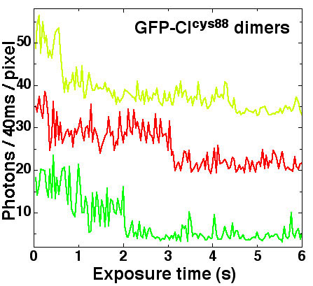
To verify that the two-step bleaching photon-emission pattern that we used to distinguish between monomers and dimers is valid, we also imaged a GFP–cI covalent dimer. Fig. 12, which is published as supporting information on the PNAS web site, shows fluorescence time traces of GFP–cI dimers, with the signature two-step bleaching pattern in each trace. Thus, the two-step bleaching is indeed the signature of a GFP dimer.

Next, we proceeded to count the number of GFP–LacI molecules bound to lacO₂₅₆. Fig. 7a shows a color image of GFP–LacI bound to lacO₂₅₆-DNA attached to a fused-silica surface. Time-averaged images of GFP–LacI and DNA were false colored to be green and red, respectively, and superimposed, so that the overlapping green and red dots indicate bound molecules. The fluorescence intensity per pixel vs. time pattern of representative bound GFP–LacI multimers is different from that of an unbound monomer (Fig. 7b); it is a continuous exponentially decreasing curve devoid of sudden photobleaching events. The exponential fit to the curve gives a GFP characteristic bleaching time constant of 0.3 s for the illumination intensity of 1,000 W/cm².

The number of bound GFP–LacI molecules was obtained by using the IPMC method, and its distribution is shown in Fig. 8. The number of bound proteins ranges from an order of 4 to an order of 100, with a mean of 13 (±6 SD). This distribution is specific to the GFP–LacI monomer/lacO concentration ratio of 6:1. When the GFP–LacI monomer/lacO ratio was increased to 18:1 by tripling the protein concentration, the number of bound GFP–LacI also increased approximately three times.

To verify that the width of the distribution is not primarily due to random GFP bleaching, we modeled the total photon yields of 13 randomly selected GFP–LacI monomers that have a Poisson photon-yield distribution (Fig. 6). The simulated distribution is shown in the Fig. 8 Inset a to have a mean of 13 and a SD of 2. This narrow distribution indicates that our measured broader distribution indeed represents a large variation in the number of bound GFP–LacI. We have also examined the effect of BOBO-3 dye on the specific binding of GFP–LacI by decreasing the dye-to-DNA ratio to one dye molecule per 100 bp. The Fig. 8 Inset b shows that the number of bound GFP–LacI is 15 ± 7 (mean ± SD), and it has approximately the same mean and SD as for one dye per 5 bp. Thus, the dye effect is negligible.

To evaluate possible quenching between GFP and BOBO-3, the number of GFP–LacI monomers bound to lacO₂₅₆-DNA was compared under two different conditions: one condition with oxygen scavenging, in which the BOBO-3 dye lasts 30 min without bleaching, and the other condition without oxygen scavenging, in which BOBO-3 bleaches within a minute under the illumination conditions of 50 W/cm². With oxygen scavenging, BOBO-3 was active while GFP was being imaged; thus, there could possibly be GFP–BOBO-3 quenching. Without oxygen scavenging, where the DNA was first imaged and the BOBO-3 dye bleached, there should be no GFP–BOBO-3 interaction. If the numbers of bound proteins under the two conditions are identical, it can be inferred that there is negligible GFP/BOBO-3 quenching, despite their overlapping spectra. Fig. 13, which is published as supporting information on the PNAS web site, demonstrates that there is no significant energy transfer between GFP and BOBO-3.

It is clear that there are only of order 10 GFP–LacI monomers bound to the 256 tandem lacO, despite the potential 500 monomer capacity at our nanomolar protein concentrations. Fig. 1c shows the sparsely bound density GFP–LacI on DNA. This low occupancy level of 2.5% was unexpected.

We also studied the effect of the inducer IPTG on LacI–DNA interaction, in part to verify that the observed bindings are specific. It is generally believed that IPTG binds to LacI and releases it from its associated DNA. We measured the number of bound GFP–LacI molecules after adding 1 mM IPTG to the LacI–DNA–BOBO-3 solution; the mean number decreased by ≈60% from 19 to 8 (Fig. 9). This mean number of molecules is significantly higher than expected for the 1 mM concentration of IPTG, in which most, if not all, of the bound proteins should be dissociated. This mean value is the same for measurements performed a few minutes to a few hours after adding IPTG. Premixing 1 mM IPTG with GFP–LacI for 1 h before adding DNA gave a similar mean of seven bound proteins. One possible explanation for this result is that the binding coefficient of LacI to a tandem array of binding sites is a function of the number of bound proteins N, most likely a declining function with 1/N.

Fig. 9.

The number of GFP–LacI bound to lacO₂₅₆–DNA for three different conditions: without IPTG, with 1 mM IPTG added after the LacI–DNA–BOBO-3 binding, and with 1 mM IPTG preincubated with GFP–LacI for 1 h before adding DNA and BOBO-3 dye. The numbers of bound GFP–LacI are 19 ± 13, 8 ± 5, and 7 ± 3 (mean ± SD), respectively.

LacI-DNA in Nanochannels. Another method of verifying the specific binding, and the distribution of proteins along the lacO₂₅₆ sequences, is to localize the bound proteins along DNA.

Fig. 10a is a time-averaged image of GFP–LacI bound to lacO₂₅₆-DNA elongated in a nanochannel. There are ≈20 GFP–LacI bound to the operator sequence in this image. The fit for DNA using Eq. 2 gives the DNA length L_zD = 4.9 μm(σ₀ = 175 nm, σ_f1 = 800 nm, and σ_f2 = 87 nm); the fit for LacI–lacO₂₅₆ gives the protein–DNA length L_zp = 1.1 μm (Fig. 10b). The fractional center location of the LacI–lacO₂₅₆ is 0.40 and agrees with that of lacO₂₅₆ of 0.32. The fractional length of the LacI–lacO₂₅₆ is L_zp/L_zD = 0.22, and agrees with that of lacO₂₅₆ of lacO₂₅₆/L_c = 9.2/42.05 kbp = 0.22. This result indicates that the 20 GFP–LacI proteins were distributed across the entire lacO₂₅₆ sequence. The length of the lacO segment is unaffected by the bound proteins, and, thus, we infer that the binding of 20 LacI does not obviously affect global DNA properties, such as persistence length.

Fig. 10.

LacI bound to DNA in a nanochannel. (a) Time-averaged image of GFP–LacI bound to lacO₂₅₆–DNA elongated in a 150 × 200 nm channel. There are ≈20 GFP–LacI molecules bound to this lacO₂₅₆–DNA molecule. This molecule traveled from right to left into the nanochannel driven by an electric field of 5V/50 μm. (b) Fluorescence intensity profiles for the DNA and the bound GFP–LacI. The fits are dashed lines.

An example with ≈24 GFP–LacI bound to lacO₂₅₆–DNA was studied to obtain the protein-distribution statistics (Fig. 11). The data points cluster around the fractional center position of 0.32 and the fractional length of 0.22 of the pristine lacO₂₅₆. Thus, we infer that most, if not all, proteins were bound specifically. By correlating the number of bound proteins with the measured LacI–lacO₂₅₆ length, we observed that when only a few bound proteins were present, they appeared as single dots distributed randomly along the lacO₂₅₆ sequence. However, for >10 bound proteins, they occupied more sites along lacO₂₅₆ sequence, which to our optical system appeared to take up the whole 1.1-μm-long lacO₂₅₆ (Fig. 10). At our optical resolution of ≈300 nm, we cannot clearly resolve more than two protein clusters. Because almost all observed proteins were on the expected lacO₂₅₆ sites, we infer that there were very few nonspecific binding events in these images.

Fig. 11.

Fractional center locations and fractional lengths of LacI–lacO₂₅₆ for 24 different samples. The center position is the fractional distance from the center of the LacI-bound DNA to the shorter end of the DNA molecule. The dashed lines mark the fractional center position of 0.32 and the fractional length of 0.22 of the native lacO₂₅₆ length.

Conclusions

We have demonstrated the direct imaging of GFP–LacI proteins bound to DNA with tandem lacO insertions. The number of bound molecules was counted by using an IPMC method, and the locations of the bound proteins were determined. An unexpected finding is that only 2.5% of the sites are occupied. The simplest model that might explain such a “long-range” interaction is the nonlinear way that strain energy induced by bending or twisting of the DNA helix upon transcription factor binding influences binding further (20); the strain energy varies as the square of the twisting angle or bending radius. If two transcription factors bind next to each other, the induced strain energy could increase by a factor of 4 and strongly inhibit neighboring occupation. The IPMC method, if properly applied to other fluorescence marker systems, can be a powerful tool to count molecules that cannot be resolved optically. In conjunction with localizing the bound proteins on DNA by the use of nanochannels or other methods, we are one step closer to imaging protein–DNA interactions in real time. Only then can we answer some of the most fundamental protein–DNA interaction questions, such as the binding mechanism of proteins to their recognition-specific sites.

References

- 1.Jacob, F. & Monod, J. J. (1961) J. Mol. Biol. 3, 318–356. [DOI] [PubMed] [Google Scholar]
- 2.Lewis, M., Chan, G., Horton, N. C., Kercher, M. A., Pace, H. C., Schumacher, M. A., Brennan, R. G. & Lu, P. (1996) Science 271, 1247–1254. [DOI] [PubMed] [Google Scholar]
- 3.Kalodimos, C. G., Biris, N, Bonvin, A. M. J. J., Levandoski, M. M., Guennuegues, M., Boelens, R. & Kaptein, R. (2004) Science 305, 386–389. [DOI] [PubMed] [Google Scholar]
- 4.Bell, C. E. & Lewis, M. (2000) Nat. Struct. Biol. 7, 209–214. [DOI] [PubMed] [Google Scholar]
- 5.Levandoski, M. M., Tsodikov, O. V., Frank, D. E., Melcher, S. E., Saecker, R. M. & Record, M. T., Jr. (1996) J. Mol. Biol. 260, 697–717. [DOI] [PubMed] [Google Scholar]
- 6.Fumin, D., Stefanie, S., Olav, Z., Brigitte, K.-W., Benno, M.-H. & Andrew, B. (1999) J. Mol. Biol. 290, 653–666.10395821 [Google Scholar]
- 7.Straight, A. F., Belmont, A. S., Robinnett, C. C. & Murray, A. W. (1996) Curr. Biol. 6, 1599–1608. [DOI] [PubMed] [Google Scholar]
- 8.Robinett, C. C., Straight, A., Li, G., Willhelm, C., Sudlow, G., Murray, A. & Belmont, A. S. (1996) J. Cell Biol. 135, 1685–1700. [DOI] [PMC free article] [PubMed] [Google Scholar]
- 9.Yang, F., Moss, L. G. & Phillips, G. N. (1996) Nat. Biotechnol. 14, 1246–1251. [DOI] [PubMed] [Google Scholar]
- 10.Straight, A. F., Sedat, J. W. & Murray, A. W. (1998) J. Cell Biol. 143, 687–694. [DOI] [PMC free article] [PubMed] [Google Scholar]
- 11.Chen, J. & Matthews, K. (1994) Biochemistry 33, 8728–8735. [DOI] [PubMed] [Google Scholar]
- 12.Schmitz, A., Coulondre, C. & Miller, J. H. (1978) J. Mol. Biol. 123, 431–456. [DOI] [PubMed] [Google Scholar]
- 13.Kishino, A. & Yanagida, T. (1988) Nature 334, 74–76. [DOI] [PubMed] [Google Scholar]
- 14.Madou, M. J. (2002) Fundamentals of Microfabrication: The Science of Miniaturization (CRC Press, Boca Raton, FL), 2nd Ed.
- 15.Tegenfeldt, J., Prinz, C., Cao, H., Chou, S., Reisner, W., Riehn, R., Wang, Y. M., Cox, E. C., Sturm, J., Silberzan, P. & Austin, R. (2004) Proc. Natl. Acad. Sci. USA 101, 10979–10983. [DOI] [PMC free article] [PubMed] [Google Scholar]
- 16.Pierce, D. W., Hom-Booher, N. & Vale, R. D. (1997) Nature 388, 338–338. [DOI] [PubMed] [Google Scholar]
- 17.Dickson, R. M., Cubitt, A. B., Tsien, R. Y. & Moerner, W. E. (1997) Nature 388, 355–358. [DOI] [PubMed] [Google Scholar]
- 18.Kubitscheck, U., Kuckmann, O., Kues, T. & Peters, R. (2000) Biophys. J. 78, 2170–2179. [DOI] [PMC free article] [PubMed] [Google Scholar]
- 19.Chiu, C.-S., Kartalov, E., Unger, M., Quake, S. & Lester, H. A. (2001) J. Neurosci. Methods 105, 55–63. [DOI] [PubMed] [Google Scholar]
- 20.Hogan, M. E. & Austin, R. H. (1987) Nature 329, 263–266. [DOI] [PubMed] [Google Scholar]
Associated Data
This section collects any data citations, data availability statements, or supplementary materials included in this article.