Machine learning-based estimation of crude oil-nitrogen interfacial tension

Abstract

Accurate estimation of interfacial tension (IFT) between nitrogen and crude oil during nitrogen-based gas injection into oil reservoirs is imperative. The previous research works dealing with prediction of IFT of oil and nitrogen systems consider synthetic oil samples such n-alkanes. In this work, we aim to utilize eight machine learning methods of Decision Tree (DT), AdaBoost (AB), Random Forest (RF), K-nearest Neighbors (KNN), Ensemble Learning (EL), Support Vector Machine (SVM), Convolutional Neural Network (CNN) and Multilayer Perceptron Artificial Neural Network (MLP-ANN) to construct data-driven intelligent models to predict crude oil – nitrogen IFT based upon experimental data of real crude oils samples encountered in underground oil reservoirs. Several statistical indices and graphical approaches are used as accuracy performance indicators. The results show that virtually all the gathered datapoints are suitable for the purpose of model development. The sensitivity analysis indicated that pressure, temperature and crude oil API all negatively affect the IFT, with pressure being the most effective factor. The evaluation study proved that Random Forest is the most accurate developed intelligent model as it was characterized with acceptable R-squared (0.959), mean square error (1.65), average absolute relative error (6.85%) of unseen test datapoints as well as with correct trend prediction of IFT with regard to all input parameters of pressure, temperature and crude oil API. The developed model can be considered an accurate an easy-to-use tool for the prediction of crude oil/N₂ IFT values for enhance oil recovery study optimization and upstream reservoir investigations.

Supplementary Information

The online version contains supplementary material available at 10.1038/s41598-025-85106-y.

Introduction

The inefficacy of oil retrieval during primary and secondary production stages has engendered an accelerated maturation of numerous methods for the reduction of residual oil saturation antecedent to the permanent discontinuation of oil reservoir operation^1,2. For the purpose of augmenting oil recovery, the introduction of gas into oil reservoirs has proven to be a widely adopted practice, facilitating an enhancement of oil retrieval through the injection of an assortment of gaseous media, namely, natural gas, enriched natural gas, carbon dioxide, nitrogen, or flue gas^3,4. Within the spectrum of available gas types, carbon dioxide has garnered recognition as a particularly efficacious means of facilitating enhanced oil recovery, primarily via viscosity diminution, vaporization, and miscible displacement, thereby effectuating the evacuation of oil from the reservoir⁵. As a dual-purpose strategy, the employment of CO₂ for enhanced oil recovery (EOR) not only promotes the retrieval of crude oil but also enables the sequestration of CO₂, thereby reducing greenhouse gas emissions. Notwithstanding its numerous advantages, the CO₂ flooding technique is beset with a host of economic and technical challenges. From a technical standpoint, asphaltene precipitation during CO₂ injection can prove to be a substantial impediment to the efficacy of this method, engendering grave issues such as reservoir impairment, alteration of wettability, diminution of relative permeability, and obstruction of flow in the reservoir and surface facilities. Consequently, in certain oil fields, the implementation of CO₂ is deemed impracticable due to the prospect of asphaltene precipitation. Other obstacles encountered in the course of CO₂ flooding include corrosion, freezing of the wellbore annulus, poor injectivity, and pump-related difficulties. From an economic perspective, the key considerations are oil price, capital expenditure, and operational cost. However, paramount to all economic and technical concerns is the availability, abundance, accessibility, and reliability of the CO₂ source^5–8.

In light of the aforementioned impediments potentially encountered during CO₂ injection, certain companies are disinclined to utilize CO₂ as an injection gas. Consequently, nitrogen injection is proffered as a non-hydrocarbon source of gas for the displacement of crude oil from matured oil reservoirs. The mechanisms by which nitrogen can effectuate oil displacement in this context include pressure maintenance, gravity enhancement, immiscible displacement, miscible displacement, and functioning as a driver for miscible slug. In the context of miscible displacement, nitrogen can efficaciously displace crude oil by inducing the formation of a miscible bank through vaporization of the intermediate components of the oil, thereby facilitating the development of miscibility^9–11. When the interfacial tension (IFT) between two phases reaches ultralow values, it indicates that the phases have achieved miscibility. Consequently, estimating the IFT can provide valuable insights into the miscibility status of the phases. Therefore, having reliable tools for accurate estimation of IFT between crude oil and gases deems to be necessary mostly because experimental workflows to measure IFT are heavy, tedious, arduous, time-consuming and costly. This need is more pronounced when one involves gas injection based EOR methods such as carbon dioxide and nitrogen injection methods, though the minimum miscibility pressure of nitrogen/crude oil system is known to be much larger than that of carbon dioxide/crude oil system. Indeed, having reliable and simple models to accurately compute IFT between crude oil and gas systems is vital for upstream reservoir studies and EOR optimization investigations.

Machine learning and artificial intelligence methods have been proved as efficient, accurate and reliable tools for the prediction tasks^12–15. Bahaloo et al.¹⁶ conducted a review to explore how machine learning and artificial intelligence can be implemented in petroleum industry to enhance upstream processes like drilling, reservoir studies, and production engineering areas. Agwu et el¹⁷. created a neural network model to forecast oil flow rates in wells operated by electrical submersible pumps. Alatefi et al.¹⁸ introduced multiple artificial models to estimate minimum miscibility pressure of carbon dioxide. Alatefi et al.¹⁹ provided a combinational method based upon conventional well logs, machine learning methods and core analysis to precisely predict porosity of carbonate formations. Alatefi and Almeshal²⁰ made use of real field Pressure–Volume–Temperature (PVT) data to precisely estimate bubble point pressure of oil-bearing reservoirs. Hadavimoghaddam et al.²¹ accurately predicted solubility of hydrogen in hydrocarbon fuels using white box machine learning methods. Youcefy et al.²² predicted stand pipe pressure via a machine learning model in real time. Hassaan et al.²³ put forth a new way to estimate rock permeability and porosity for the sake of reservoir evaluation based upon different machine learning methods. Lv et al.²⁴ predicted the carbon dioxide diffusion coefficient into heavy crude oil/bitumen. Lv er al²⁵ provided powerful machine learning models to accurately forecast the values of minimum miscibility pressure for crude oil/carbon dioxide systems.

For the purpose of studies with regard to miscible displacement via nitrogen gas, accurate models to predict IFT between nitrogen and crude oil phases are deemed to be vital. In this regard, Salehi et al.²⁶ accurately modeled IFT between n-alkanes and mixtures of carbon dioxide and nitrogen gases using machine learning methodologies. Mahdaviara et al.²⁷ put forward machine learning based models for the prediction task of n-alkanes and gas mixtures (containing nitrogen, methane and carbon dioxide) IFT values. Kalam et al.²⁸ also provided artificial intelligence based techniques to easily predict IFT between nitrogen/carbon dioxide mixtures and normal alkanes. Ameli et al.²⁹ performed the same task using several data-driven techniques. Zhang et al.³⁰ put forth a novel supervised machine learning methodology for the quick forecast of nitrogen-alkanes IFT.

As can be pinpointed, all the previous research works dealing with prediction of IFT of oil and gas phase consider synthetic oil (particularly, n-alkanes) whereas taking into consideration the realistic conditions occurring in real underground petroleum reservoirs, crude oil prevails. This study, therefore, aims at providing machine leaning models to predict nitrogen-crude oil IFT as a function of temperature, pressure and crude oil API. Eight machine learning methods including Decision Tree (DT), AdaBoost (AB), Random Forest (RF), K-nearest Neighbors (KNN), Ensemble Learning (EL), Support Vector Machine (SVM), Convolutional Neural Network (CNN) and Multilayer Perceptron Artificial Neural Network (MLP-ANN) are specifically utilized for the purpose of intelligent model development. A dataset gained from previously published experimental studies is used although before model construction, its reliability is checked using Leverage outlier detection methodology. To gain more insights also, sensitivity studies are carried out in order to comprehend the relative effects of different parameters on the nitrogen-crude oil IFT. The created data-driven models are assessed using disparate statistical and graphical approaches. The main factor that differentiates this research work with its previous counterparts is the development of machine learning based upon real crude oil samples which is in realistic encountered in reservoir studies.

Data gathering and models’ evaluation indices

This research incorporates an experimental database consisting of 148 datapoints, gathered from an extensive review of previously published literature^9,31–35, where significant work was devoted to the experimental measurement of the equilibrium IFT between crude oil and nitrogen gas across various pressure, temperature and crude oil API values. The statistical details related to all experimental data used for the model development are organized in Table 1.

Table 1.

Statistical data with regard to experimental IFT dataset.

Parameter	Minimum	Maximum	Average	Standard deviation
P (MPa)	0.48	51.77	15.90	12.12
T(K)	295.15	403.15	342.65	28.69
API Gravity	20.20	42.55	26.20	7.048
IFT (mN/m)	3.78	25.50	14.89	5.47

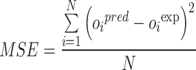
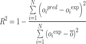
To compare the predictive capabilities of each developed model, several performance metrics are calculated for each model, as outlined below^36,37:

1

2

3

4

In which RE%, AARE%, MSE, and R² stand for relative error percent, average absolute relative error percent, mean square error, and coefficient of determination. Also, subscript i represents the index number of a given data point within the dataset, while pred and exp denote the estimated and actual data points, respectively. Additionally, N symbolizes the total number of data points in the dataset.

Notice that the input variables include crude oil API, temperature and pressure while equilibrium IFT is the output variable when constructing the predictive models. In additions, three datasets, namely training, validation and testing are randomly generated. The train, validation and test datasets contain 80% and 10% and 10%, respectively, of the total gathered datapoints. It is crucial to highlight that input and output variables are initially normalized using the following equation, aiming to minimize the effects of variations within the datasets:

5

In the provided equation, the symbols n, n_max, n_min, and n_norm denote the actual data point, the maximum value in the dataset, the minimum value in the dataset, and the normalized data point, respectively. This normalization process ensures a more accurate comparison of model performance by mitigating the influence of inherent data variability.

As mentioned before, seven machine learning methods including Decision Tree (DT), AdaBoost (AB), Random Forest (RF), K-nearest Neighbors (KNN), Ensemble Learning (EL), Support Vector Machine (SVM), Convolutional Neural Network (CNN) and Multilayer Perceptron Artificial Neural Network (MLP-ANN) are utilized for the construction of robust data-driven models. The backgrounds of the aforementioned methods are given in the appendix. Notice that we selected these machine learning algorithms to capture the complexity of interfacial tension in crude oil-nitrogen systems. The chosen models encompass both interpretable and complex learners, ensuring a comprehensive approach to identifying non-linear relationships and feature interactions inherent to the dataset. Decision Tree (DT) and Random Forest (RF) were chosen for their robustness in handling non-linear data, with Random Forest’s ensemble approach effectively reducing variance. AdaBoost (AB), another ensemble method, enhances model accuracy by iteratively focusing on challenging instances, a benefit when capturing finer nuances of interfacial tension. K-Nearest Neighbors (KNN) complements these with its non-parametric structure, ideal for local variations without assuming data distribution. Additionally, Support Vector Machine (SVM) and neural network-based models, including Convolutional Neural Network (CNN) and Multilayer Perceptron (MLP-ANN), were chosen for their ability to learn complex patterns. SVM’s kernel functions allow it to manage intricate decision boundaries, whereas CNN’s spatial learning capabilities make it uniquely suited to capture nuanced feature interactions. MLP-ANN, known for its universal approximation capabilities, supports these findings by mapping non-linear dependencies. Finally, ensemble learning provides a well-rounded estimate by integrating these individual models, thereby balancing interpretability and predictive power for reliable estimation of crude oil-nitrogen interfacial tension.

Results and discussion

Outlier detection

The Leverage method serves as a means to identify data points with significant deviations. Its core principle relies on the combination of standardized residuals and the Hat matrix (H). The Hat matrix is calculated using the following formula³⁸:

6

In the provided equation, X symbolizes a matrix with dimensions n and m, representing the number of input parameters and data points, respectively. Moreover, X^T denotes the transpose of matrix X. The hat value for a given data point is calculated using the diagonal elements of the Hat matrix. The warning Leverage (H*) can be determined using the following formula³⁸:

7

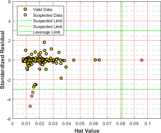
In this equation, m and n correspond to the previously defined matrix dimensions representing the number of input parameters and data points, respectively. By assessing hat values in relation to H*, the Leverage method enables the identification of potential outliers or influential points within the dataset. Subsequently, the identification of questionable data points is achieved by establishing trustworthy and suspect zones within the Williams’ plot. As illustrated in Fig. 1, suspect and leverage limits serve to demarcate the reliable region. A significant portion of interfacial tension data points reside within the reliable zones, while only 4 datapoints (highlighted in red) are categorized as suspect IFT values. This visual representation facilitates the evaluation of data quality and the potential impact of suspect datapoints on subsequent modeling and analysis efforts. Notice that to create generalizable methods, all datapoints are considered for the model development here. Notice that the outliers were found using the methodology given above and the experimental dataset in this study.

Fig. 1.

Outlier detection within the experimental dataset.

Sensitivity analysis

In this segment, our endeavor shall focus upon ascertaining the proportional influence of each respective input variable - viz., temperature, pressure and crude oil API - upon the resultant crude oil – nitrogen gas equilibrium IFT. This shall be effectuated with cognizance of the respective relevancy factor for each individual input variable. The equation for the relevancy factor is thusly defined as³⁸:

8

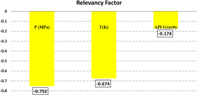
Herein, the identifier “j” refers to the discrete input variable under consideration. Note that the conceivable scope of the relevancy factor is delimited to the interval − 1 to + 1. Moreover, the magnitude of the computed relevancy factor is directly proportional to the strength of the correlation between the input and output variables. A negative relevancy index denotes an inverse correlation, while a positive index signifies a direct correlation. The computed relevancy factors for each of the input variables under consideration are presented in Fig. 2. As can be seen, all the input variables such as pressure, temperature and API gravity inversely affect the IFT between crude oil and nitrogen gas. In addition, pressure is the highly effective parameter amongst all the parameters with a relevancy factor of -0.752.

Fig. 2.

The computed relevancy factor for each input factor.

Models’ hyperparameter determination

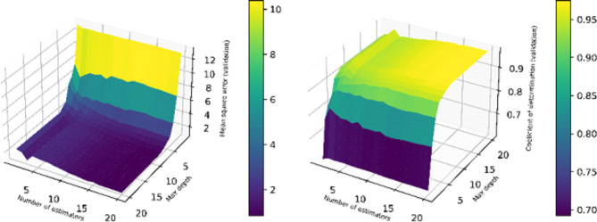
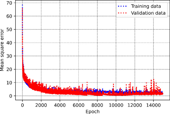
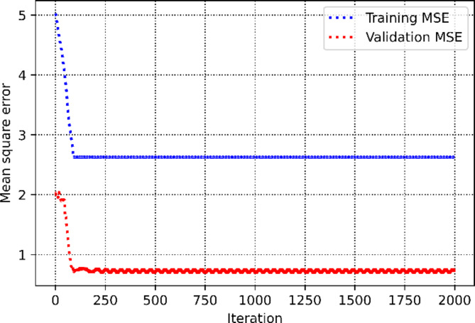
This section discusses the process of obtaining hyperparameters. Figure 3 illustrates the relationship between the coefficient of determination and mean square error versus the maximum depth hyperparameter within the Decision Tree method. It is evident that the optimal value is determined to be 8. Similarly, the value of 5 is also identified as the optimal number of estimators for the AdaBoost machine learning method, as shown in Fig. 4. Figure 5 presents two 3D plots depicting the mean square error and coefficient of determination during the validation phase of the Random Forest approach. The optimum values for the maximum depth and number of estimators are found to be 20 and 19, respectively. Figure 6 depicts mean square error and determination coefficient versus number of neighbors in KNN approach, in which it is shown the optimum number of neighbors is 2. Furthermore, the optimized value of the SVM hyperparameter (C) is estimated to be 701, as depicted in Fig. 7. Figures 8 and 9 shows the tuning process of the MLP-ANN and CNN methods in terms of mean square error versus iteration during the training and validation phases. As can be seen, the plots for Decision Tree, Adaptive Boosting, and Support Vector Machine all suffers from overfitting issues as large discrepancy can be vividly observed in the MSE metric of training and validation phase.

Fig. 3.

The process of obtaining the optimum value for max depth in terms of mean square error and determination coefficient versus max depth in DT algorithm.

Fig. 4.

The process of obtaining the optimum value for number of estimators in terms of mean square error and determination coefficient versus number of estimators in AdaBoost algorithm.

Fig. 5.

The process of obtaining the optimum value for number of estimator and max depth in terms of mean square error and determination coefficient versus these parameters in RF algorithm.

Fig. 6.

The process of obtaining the optimum value for number of neighbors in terms of mean square error and determination coefficient versus number of neighbors in KNN algorithm.

Fig. 7.

The process of obtaining the tuning parameter of SVM approach in terms of mean square error and determination coefficient versus c hyperparameter in SVM approach.

Fig. 8.

The process of optimizing CNN approach.

Fig. 9.

The process of optimizing MLP-ANN approach.

Table 2 tabulates the tuning parameters (range and their found optimum values) for each of the machine learning algorithms used in this study. Note that we used the “averaging mode” of the Ensemble Learning machine learning algorithm, with its base estimators as Decision Tree, Adaptive Boosting, Random Forest, and K-nearest Neighbors each of which with their tuned hyperparameters.

Table 2.

Range and tuned values of hyperparameters of all the machine learning methods utilized in this study.

Method	Parameters and the range	Optimum values and structure
DT	• Max depth (ranged 1 to 50) • Min samples split (ranged 2 to 20) • Min samples leaf (range 1 to 20)	• Max depth: 8 • Min samples split: 2 • Min samples leaf: 1
AB	• Number of estimators (ranged 1 to 50) • Learning rate (0.01 to 1.0)	• Number of estimators: 5 • Learning rate: 10
RF	• Number of estimators (ranged 1 to 20) • Max depth (ranged 1 to 20) • Min sample split (ranged 2 to 20)	• Number of estimators: 19 • Max depth: 20 • Min sample split: 2
KNN	• Number of neighbors (ranged 1 to 50)	• Number of neighbors: 2
EL	• Constructed based upon DT, AB, RF an KNN algorithms	• Tuned values of each DT, AB, RF an KNN methods
SVM	• C hyperparameter (ranged 1 to 1000) • Kernel function (linear, polynomial, RBF, Sigmoid) • Gamma (range 1e-4 to 1.0)	• C hyperparameter: 701 • Kernel function: RBF • Gamma: 0.33
CNN	• Number of filters (ranged 32 to 512) • Filter size (3*3, 5*5 and 7*7) • Pooling size (2*2 or 3*3)	• Number of filters: 32 • Filter size: 5*5 • Pooling size: 2*2
MLP-ANN	• Number of hidden layers (ranged 2 to 20) • Number of neurons in each hidden layer (ranged 5 to 40) • Activation function (relu, tanh, sigmoid) • Learning rate (ranged 0.001 to 0.1)	• Number of hidden layers: 6 • Number of neurons in each hidden layer: 33 • Activation function: relu • Learning rate: 0.001

Models’ evaluation

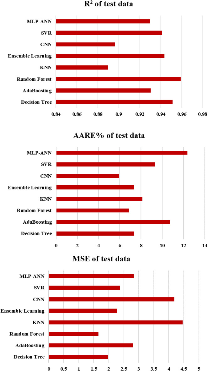
Table 3 presents the evaluation indices, including the coefficient of determination, mean square error, and average absolute relative error (AARE%), for the developed data-driven intelligent models such as Decision Tree, AdaBoost, Random Forest, Ensemble Learning, K-nearest Neighbors, Support Vector Machine, Convolutional Neural Network (CNN) and Multilayer Perceptron Artificial Neural Network (MLP-ANN). Additionally, to enhance the evaluation process, these parameters for the testing phase are illustrated in Fig. 10.

Table 3.

Statistical indices with regard to training, validation and testing phases for all the developed intelligent models.

Model	R 2			MSE			AARE%
	Training	Validation	Test	Training	Validation	Test	Training	Validation	Test
Decision Tree	0.998628	0.9419383	0.951227	0.038274	1.9598029	1.969701	0.619965	5.9495814	7.373993
AdaBoost	0.994503	0.9829023	0.930396	0.153343	0.5771109	2.810983	1.385973	4.2744479	10.70054
Random Forest	0.962907	0.9752893	0.959012	1.034649	0.834079	1.655327	4.382448	5.2276914	6.855313
KNN	0.943946	0.9767881	0.889473	1.563539	0.7834898	4.463694	4.801762	3.9701605	8.125265
Ensemble Learning	0.990196	0.981191	0.943542	0.273472	0.6348763	2.280067	2.304018	4.1129071	7.342033
CNN	0.939171	0.9418796	0.896304	1.696726	1.9617828	4.187813	5.075706	5.2224487	5.948077
SVR	0.915223	0.9957063	0.941175	2.364719	0.1449279	2.375694	5.240866	1.78921	9.307926
MLP-ANN	0.905727	0.9776783	0.929881	2.629609	0.7534436	2.831794	8.442734	3.8741063	12.3595

Fig. 10.

AARE%, MSE and R-squared values for the testing phase of all the developed models in this study.

As observed with regard to test data, the Random Forest and Decision Tree methods exhibit the lowest mean square error, indicating their superior performance in predicting the IFT. Furthermore, these methods achieve the highest values of the determination coefficient. Conversely, for the prediction of IFT in this study, KNN and CNN appear to be less accurate, as they have the highest values of MSE and AARE% and the lowest values of the determination coefficient. Notice that Decision Tree and Ensemble Learning suffers from overfitting as evidenced by the large discrepancy in MSE between training/test or training/validation segments.

To evaluate the performance of the trained algorithms and examine their estimation accuracy, this study employs several visual plots. Initially, cross plots for all proposed models are generated, as depicted in Fig. 11. For both the Random Forest and Decision Tree models, the clustering of points around the unit slope line signifies a high level of accuracy. Moreover, the equations derived from the fitting lines on these points are notably close to the bisector line. Additionally, the distribution of relative deviation for each estimator is shown in Fig. 12. A closer alignment of the data with the y = 0 line indicates higher estimator accuracy. According to this plot and considering the overfitting issue of Decision Tree method, the Random Forest algorithm is identified as the most effective predictive tool.

Fig. 11.

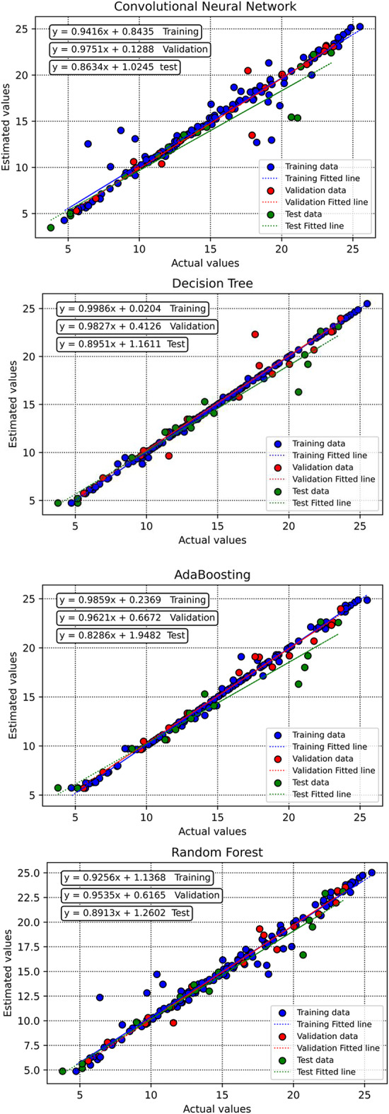
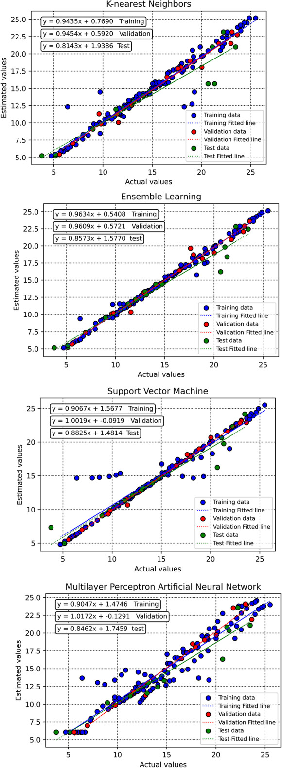
Cross plots of actual versus estimated values for all the developed models in this study.

Fig. 12.

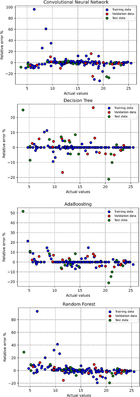
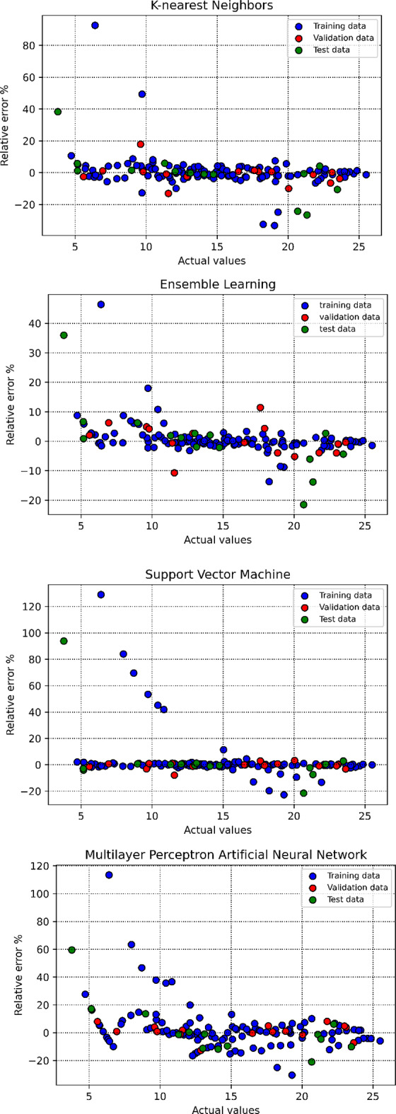
Relative error % versus actual values for all the developed models in this study.

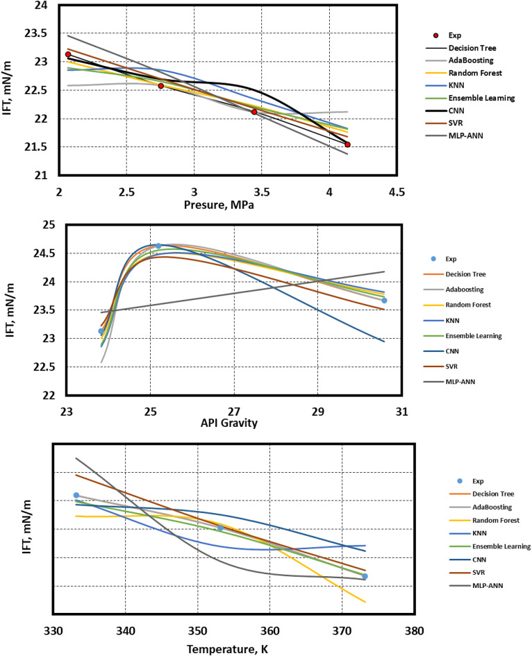
As another testing method to assess the reliability of the developed models, trend prediction should be considered, for which case, it is indicated in Fig. 13 for different input parameters of pressure, temperature and crude oil API. In terms trend prediction of pressure, KNN, CNN and AdaBoost fails to accurately capture the correct trend, while for API gravity, MLP-ANN is unable to capture the correct trend. Finally, KNN fails to in correctly predicting the trend prediction of IFT versus temperature. Therefore, considering the trend prediction, all evaluation metrics as well as the overfitting issue, we can conclude that combining the results from the trend prediction and the evaluation indices elucidated earlier, Random Forest is the most accurate developed intelligent model to predict crude oil-nitrogen IFT in terms of pressure, temperature and crude oil API.

Fig. 13.

Trend prediction ability of the developed data-driven models in terms of temperature, pressure and crude oil API.

Study limitations, practical application, and future recommendations

A key limitation of this study lies in the dataset size, which may impact the generalizability and robustness of the findings. While complex models such as CNN are employed to explore hierarchical relationships in feature data, the limited data size introduces a risk of overfitting, where the model might capture noise rather than genuine patterns. Furthermore, the databank may lack diversity, potentially limiting the model’s applicability across different conditions or crude oil compositions, thus affecting its external validity. For future research, expanding the dataset to include a broader range of crude oil compositions, nitrogen levels, and environmental conditions is recommended to improve model robustness and generalizability. Where dataset expansion is constrained, transfer learning may offer a feasible approach to apply complex models effectively by building on pretrained models from similar domains. Additionally, future studies could explore alternative machine learning models and optimization techniques, such as hyperparameter tuning and ensemble methods, to improve performance while maintaining interpretability. Testing on external datasets would also be essential to confirm the model’s applicability beyond the initial study conditions, thereby strengthening its real-world relevance. These remain to be investigated by our research group during our future works.

Despite these limitations, the developed data-driven models offer practical applications in accurately predicting interfacial tension (IFT) for nitrogen/crude oil systems, a crucial parameter in enhanced oil recovery (EOR) processes and other industry applications. Accurate IFT prediction helps in optimizing the selection of injection parameters, improving the effectiveness of nitrogen injection for EOR by enhancing oil displacement efficiency, and reducing operational costs. By providing reliable IFT estimates, the models can aid in making more informed decisions in field operations, particularly when experimental measurements are unavailable or impractical, thereby improving both safety and efficiency in real-world applications.

Conclusions

Accurate estimation of IFT between crude oil and nitrogen is vital when it comes to enhanced oil recovery optimization tasks and upstream reservoir studies. In this research work, intelligent data-driven models based on eight machine learning algorithms including Decision Tree (DT), AdaBoost (AB), Random Forest (RF), K-nearest Neighbors (KNN), Ensemble Learning (EL), Support Vector Machine (SVM), Convolutional Neural Network (CNN) and Multilayer Perceptron Artificial Neural Network (MLP-ANN) were developed to predict equilibrium interfacial tension between crude oil and nitrogen phases using an experimental dataset gathered from published works previously. The results indicated that almost all data are reliable for the purpose of data-driven model development. In addition, it was found that all the effective parameters including pressure, temperature and crude oil API inversely affect IFT, with pressure being the most effective parameter. The model evaluation using various statistical indices and graphical methods, ultimately, implied that Random Forest is the most accurately developed intelligent model to predict IFT of crude oil/nitrogen systems with acceptable R-squared (0.959), mean square error (1.65), average absolute relative error (6.85%) of unseen test datapoints. The developed model can be made use of without requiring tedious, heavy, arduous and time-consuming experimental procedures.

Electronic supplementary material

Below is the link to the electronic supplementary material.

Author contributions

Authors S.O.R., S.C., and A.K. prepared the manuscript and did the formal analysis.Authors P.P., M.A., and S.M. did the methodology.Authors B.A., M.C., M.S. and M.K. prepared the draft version of the manuscript and also edited it.

Data availability

The data that supports the finding of this study will be made available from the corresponding author upon reasonable academic request.

Declarations

Competing interests

The authors declare no competing interests.

References

- 1.Malozyomov, B. V. et al. Overview of methods for enhanced oil recovery from conventional and unconventional reservoirs. Energies16 (13), 4907 (2023). [Google Scholar]
- 2.Liu, T., Zhao, G., Qu, B. & Gong, C. Characterization of a fly ash-based hybrid well cement under different temperature curing conditions for natural gas hydrate drilling. Constr. Build. Mater.445, 137874 (2024). [Google Scholar]
- 3.Shafiei, M. et al. A comprehensive review direct methods to overcome the limitations of gas injection during the EOR process. Sci. Rep.14 (1), 7468 (2024). [DOI] [PMC free article] [PubMed] [Google Scholar]
- 4.Yu, H., Wang, H. & Lian, Z. An assessment of seal ability of tubing threaded connections: a hybrid empirical-numerical method. J. Energy Res. Technol.145 (5), 052902 (2023). [Google Scholar]
- 5.Ren, D. et al. Feasibility evaluation of CO2 EOR and storage in tight oil reservoirs: a demonstration project in the Ordos Basin. Fuel331, 125652 (2023). [Google Scholar]
- 6.Chen, P., Bose, S., Selveindran, A. & Thakur, G. Application of CCUS in India: Designing a CO2 EOR and storage pilot in a mature field. Int. J. Greenhouse Gas Control. 124, 103858 (2023). [Google Scholar]
- 7.Shen, B. et al. Interpretable knowledge-guided framework for modeling minimum miscible pressure of CO2-oil system in CO2-EOR projects. Eng. Appl. Artif. Intell.118, 105687 (2023). [Google Scholar]
- 8.Li, Z., Huang, X., Xu, X., Bai, Y. & Zou, C. Unstable coalescence mechanism and influencing factors of heterogeneous oil droplets. Molecules29 (7), 1582 (2024). [DOI] [PMC free article] [PubMed] [Google Scholar]
- 9.Hemmati-Sarapardeh, A., Ayatollahi, S., Zolghadr, A., Ghazanfari, M-H. & Masihi, M. Experimental determination of equilibrium interfacial tension for nitrogen-crude oil during the gas injection process: the role of temperature, pressure, and composition. J. Chem. Eng. Data. 59 (11), 3461–3469 (2014). [Google Scholar]
- 10.Zhang, L. et al. Pyrolytic modification of heavy coal tar by multi-polymer blending: preparation of ordered carbonaceous mesophase. Polymers16 (1), 161 (2024). [DOI] [PMC free article] [PubMed] [Google Scholar]
- 11.Fang, T., Ren, F., Wang, B., Hou, J. & Wiercigroch, M. Multi-scale mechanics of submerged particle impact drilling. Int. J. Mech. Sci.285, 109838 (2024). [Google Scholar]
- 12.Agwu, O. E., Alatefi, S., Azim, R. A. & Alkouh, A. Applications of Artificial Intelligence algorithms in Artificial Lift systems: a critical review. Flow Meas. Instrum.97, 102613 (2024). [Google Scholar]
- 13.Ghorbani, H. et al. Prediction of Heart Disease Based on Robust Artificial Intelligence Techniques. IEEE:000167 – 74 (2023).
- 14.Hajihosseinlou, M., Maghsoudi, A. & Ghezelbash, R. Regularization in machine learning models for MVT Pb-Zn prospectivity mapping: applying lasso and elastic-net algorithms. Earth Sci. Inf.17 (5), 4859–4873 (2024). [Google Scholar]
- 15.Shi, M. et al. Ensemble regression based on polynomial regression-based decision tree and its application in the in-situ data of tunnel boring machine. Mech. Syst. Signal Process.188, 110022 (2023). [Google Scholar]
- 16.Bahaloo, S., Mehrizadeh, M. & Najafi-Marghmaleki, A. Review of application of artificial intelligence techniques in petroleum operations. Petroleum Res.8 (2), 167–182 (2023). [Google Scholar]
- 17.Agwu, O. E., Alkouh, A., Alatefi, S., Azim, R. A. & Ferhadi, R. Utilization of machine learning for the estimation of production rates in wells operated by electrical submersible pumps. J. Petroleum Explor. Prod. Technol.14 (5), 1205–1233 (2024). [Google Scholar]
- 18.Alatefi, S., Agwu, O. E., Azim, R. A., Alkouh, A. & Dzulkarnain, I. Development of multiple explicit data-driven models for accurate prediction of CO2 minimum miscibility pressure. Chem. Eng. Res. Des.205, 672–694 (2024). [Google Scholar]
- 19.Alatefi, S., Abdel Azim, R., Alkouh, A. & Hamada, G. Integration of multiple bayesian optimized machine learning techniques and conventional well logs for accurate prediction of porosity in carbonate reservoirs. Processes11 (5), 1339 (2023). [Google Scholar]
- 20.Alatefi, S. & Almeshal, A. M. A new model for estimation of bubble point pressure using a bayesian optimized least square gradient boosting ensemble. Energies14 (9), 2653 (2021). [Google Scholar]
- 21.Hadavimoghaddam, F. et al. Application of advanced correlative approaches to modeling hydrogen solubility in hydrocarbon fuels. Int. J. Hydrog. Energy. 48 (51), 19564–19579 (2023). [Google Scholar]
- 22.Youcefi, M. R., Hadjadj, A. & Boukredera, F. S. New model for standpipe pressure prediction while drilling using Group Method of Data Handling. Petroleum8 (2), 210–218 (2022). [Google Scholar]
- 23.Hassaan, S., Mohamed, A., Ibrahim, A. F. & Elkatatny, S. Real-time prediction of Petrophysical Properties using machine learning based on drilling parameters. ACS Omega. 9 (15), 17066–17075 (2024). [DOI] [PMC free article] [PubMed] [Google Scholar]
- 24.Lv, Q. et al. Modelling CO2 diffusion coefficient in heavy crude oils and bitumen using extreme gradient boosting and gaussian process regression. Energy275, 127396 (2023). [Google Scholar]
- 25.Lv, Q. et al. Modelling minimum miscibility pressure of CO2-crude oil systems using deep learning, tree-based, and thermodynamic models: application to CO2 sequestration and enhanced oil recovery. Sep. Purif. Technol.310, 123086 (2023). [Google Scholar]
- 26.Salehi, E. et al. Modeling interfacial tension of N2/CO2 mixture + n-alkanes with machine learning methods: application to eor in conventional and unconventional reservoirs by flue gas injection. Minerals12 (2), 252 (2022). [Google Scholar]
- 27.Mahdaviara, M., Amar, M. N., Ostadhassan, M. & Hemmati-Sarapardeh, A. On the evaluation of the interfacial tension of immiscible binary systems of methane, carbon dioxide, and nitrogen-alkanes using robust data-driven approaches. Alexandria Eng. J.61 (12), 11601–11614 (2022). [Google Scholar]
- 28.Kalam, S., Khan, M. R., Shakeel, M., Mahmoud, M. & Abu-khamsin, A. S. Smart algorithms for determination of Interfacial Tension (IFT) between Injected Gas and Crude Oil–Applicable to EOR projects. SPE:D011S33R02 (2023).
- 29.Ameli, F., Hemmati-Sarapardeh, A., Schaffie, M., Husein, M. M. & Shamshirband, S. Modeling interfacial tension in N2/n-alkane systems using corresponding state theory: application to gas injection processes. Fuel222, 779–791 (2018). [Google Scholar]
- 30.Zhang, J. et al. A unified intelligent model for estimating the (gas + n-alkane) interfacial tension based on the eXtreme gradient boosting (XGBoost) trees. Fuel282, 118783 (2020). [Google Scholar]
- 31.Bayat, M., Lashkarbolooki, M., Hezave, A. Z. & Ayatollahi, S. Investigation of gas injection flooding performance as enhanced oil recovery method. J. Nat. Gas Sci. Eng.29, 37–45 (2016). [Google Scholar]
- 32.Awari-Yusuf, I. O. Measurement of crude oil interfacial tension to determine minimum miscibility in carbon dioxide and nitrogen [MS thesis]. Dalhousie University, Halifax, Canada; (2013).
- 33.Heidary, S., Dehghan, A. A. & Zamanzadeh, S. M. A comparative study of the carbon dioxide and nitrogen minimum miscibility pressure determinations for an Iranian light oil sample. Energy Sour. Part a Recover. Utilization Environ. Eff.38 (15), 2217–2224 (2016). [Google Scholar]
- 34.Bahralolom, I. M. & Orr, F. M. Solubility and extraction in multiple-contact miscible displacements: comparison of N2 and CO2 flow visualization experiments. SPE. Reserv. Eng.3 (01), 213–219 (1988). [Google Scholar]
- 35.Lu, T., Li, Z., Li, J., Hou, D. & Zhang, D. Flow behavior of N2 Huff and puff process for enhanced oil recovery in tight oil reservoirs. Sci. Rep.7 (1), 15695 (2017). [DOI] [PMC free article] [PubMed] [Google Scholar]
- 36.Madani, M., Moraveji, M. K. & Sharifi, M. Modeling apparent viscosity of waxy crude oils doped with polymeric wax inhibitors. J. Petrol. Sci. Eng.196, 108076 (2021). [Google Scholar]
- 37.Bemani, A., Madani, M. & Kazemi, A. Machine learning-based estimation of nano-lubricants viscosity in different operating conditions. Fuel352, 129102 (2023). [Google Scholar]
- 38.Bemani, A., Baghban, A. & Mohammadi, A. H. An insight into the modeling of sulfur content of sour gases in supercritical region. J. Petrol. Sci. Eng.184, 106459 (2020). [Google Scholar]
Associated Data
This section collects any data citations, data availability statements, or supplementary materials included in this article.
Supplementary Materials
Data Availability Statement