Recent Advances in Human Quantitative-Trait–Locus Mapping: Comparison of Methods for Selected Sibling Pairs

Abstract

During the past few years, there has been a great deal of new work on methods for mapping quantitative-trait loci by use of sibling pairs and sibships. There are several new methods based on linear regression, as well as several more that are based on score statistics. In theory, most of the new methods should be relatively robust to violations of distributional assumptions and to selected sampling, but, in practice, there has been little evaluation of how the methods perform on selected samples. We survey most of the new regression-based statistics and score statistics and propose a few minor variations on the score statistics. We use simulation to evaluate the type I error and the power of all of the statistics, considering (a) population samples of sibling pairs and (b) sibling pairs ascertained on the basis of at least one sibling with a trait value in the top 10% of the distribution. Most of the statistics have correct type I error for selected samples. The statistics proposed by Xu et al. and by Sham and Purcell are generally the most powerful, along with one of our score statistic variants. Even among the methods that are most powerful for “nice” data, some are more robust than others to non-Gaussian trait models and/or misspecified trait parameters.

Introduction

As recently as a few years ago, there were only two primary statistical methods for QTL linkage analysis using sibships: Haseman-Elston regression (Haseman and Elston 1972) and maximum-likelihood variance-components analysis (e.g., see Amos 1994; Almasy and Blangero 1998). The Haseman-Elston method, on the one hand, was derived under the assumption of a population sample of pairs with normally distributed trait values, but the regression framework makes it quite robust to selected sampling and to non-Gaussian trait distributions (for extended discussion, see Feingold 2002). Variance-components analysis, on the other hand, has much higher power than Haseman-Elston regression under ideal conditions but is not very robust to selected sampling and deviations from distributional assumptions (for discussion, see Feingold 2001). Recently, there has been an explosion of new methods that aim to equal the power of variance-components analysis while retaining the robustness of Haseman-Elston regression. One set of new methods are the regression-based statistics, essentially improvements on the original Haseman-Elston method. New regression-based methods have been developed by Drigalenko (1998), Elston et al. (2000), Xu et al. (2000), Forrest (2001), Visscher and Hopper (2001), Sham and Purcell (2001), and Sham et al. (2002). The other set of new methods are the score statistics, based on the derivative of the usual variance-components likelihood. The three primary articles on these methods were authored by Tang and Siegmund (2001), Putter et al. (2002), and Wang and Huang (2002a), with extensions by Tang and Siegmund (2002), Wang (2002), and Wang and Huang (2002b). The new score statistics are more computationally convenient than variance components, and they can be constructed in such a way as to be robust as well.

Theoretical reviews of most of the new regression-based and score-based statistics have appeared in articles by Feingold (2001, 2002). A number of other articles have compared limited subsets of these methods by using theory or simulations—including articles by Allison et al. (2000), Palmer et al. (2000), Goldstein et al. (2001), Visscher and Hopper (2001), Zhang et al. (2001), Ghosh and Reich (2002), and Zhang et al. (2002). Despite the fact that most of the new statistics should, in theory, be appropriate for selected samples, there has been very little actual testing on such samples. In the present article and its companion (Szatkiewicz et al. 2003 [in this issue]), we undertake a comprehensive simulation-based comparison of the new statistics. We limit ourselves to sibling pairs, for simplicity, but many of the general results are applicable to larger sibships as well. We perform simulation studies using both population and selected samples and estimate the type I error and the power of each statistic. We consider 11 different trait distributions, some of them substantially non-Gaussian, and we also consider robustness of the methods to misspecification of trait parameters. Our selected samples in the present article consist of sibling pairs ascertained on the basis of at least one sibling in the top 10% of the trait distribution. We defer consideration of discordant sibling pairs to the companion article (Szatkiewicz et al. 2003 [in this issue]), because of important statistical differences between samples ascertained on the basis of a single individual and samples ascertained on the basis of more than one individual.

Methods

Statistics Considered

Here, we briefly define the 12 QTL-mapping statistics that we consider in the present article. More detailed description of the statistics can be found in the reviews by Feingold (2001, 2002), as well as in the original articles cited below.

Some notation and definitions are common to all of the statistics. Let π_i be the estimated mean identity-by-descent (IBD) sharing for sibling pair i; π_i takes the value 0,  1/2, or 1 for a fully informative pair but can take intermediate values if multipoint estimates are used. Let Y_iD=(x_i1-x_i2)² be the squared trait difference for sibling pair i. Analogously, let Y_iS=[(x_i1-μ)+(x_i2-μ)]² be the mean-corrected squared trait sum. The regression of Y_iD on π_i produces a slope estimate. We define negative one times this slope estimate as and let be the slope estimate from a regression of Y_iS on π_i. Under population sampling, and are estimates of the same parameter (Drigalenko 1998). This slope parameter should be 0 under the null hypothesis of no linkage and should be positive (as we have defined the sign) under the alternative hypothesis. The first eight methods described below are based on different methods of combining the information from these two regressions.

Original Haseman-Elston (ORIGINAL.HE)

The method of Haseman and Elston (1972) simply regresses Y_iD on π_i and estimates the slope, which is equivalent to −. A negative estimate suggests that the trait is linked to the locus marker. A one-sided t test is used to test for any significant departure from 0.

Trait-sum regression (TRAIT.SUM)

For comparison to the other statistics, we include the one-sided t test based on the regression of Y_iS on π_i, although we do not expect this statistic to be particularly powerful.

Trait-product regression (TRAIT.PRODUCT)

Drigalenko (1998) suggested doing the two regressions described above and averaging the two slope estimates—or, equivalently, doing a single regression with the mean-corrected trait product, (X_i1-μ)(X_i2-μ), as the dependent variable. This method was further developed by Elston et al. (2000). We consider the one-sided t test based on the trait-product regression.

Forrest’s method (FORREST)

Rather than a simple average of the two regression slope estimates, it is more statistically desirable to use an average that is weighted by the variances of the estimates. Forrest (2001) suggested a test based on the weighted average

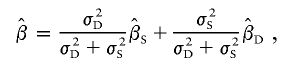where σ²_S and σ²_D are the variances of and . These weights are optimal under the assumption that the covariance, σ²_DS, of is 0, which is true for a population sample from a normal distribution but which is not necessarily true otherwise (Feingold 2002). FORREST estimates all the parameters simultaneously, using iterative least squares.

Visscher and Hopper’s method (V&H)

Visscher and Hopper (2001) proposed a test based on the same weighted slope estimate as Forrest (2001) but with the variances, σ²_S and σ²_D, estimated separately, by performing the two regressions separately.

Xu et al.’s method (XU)

Xu et al. (2000) proposed a method very similar to that of Forrest (2001) and Visscher and Hopper (2001), but their weighted average slope allows for a nonzero covariance between and , using the formula

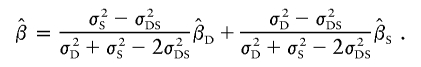Xu et al. estimate the parameters by performing the two regressions separately, similar to V&H. The covariance can be estimated by combining the residuals of the two regressions.

Sham and Purcell’s method (S&P1)

The variances σ²_D and σ²_S can actually be calculated analytically as functions of the sibling trait correlation, r, under traditional QTL models. Sham and Purcell (2001) proposed taking advantage of this, rather than estimating the variances from data as in FORREST, V&H, and XU. The primary method outlined by Sham and Purcell (2001) regresses the dependent variable

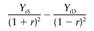on π_i, where the trait values x_i1 and x_i2 are standardized to have a variance of 1 before calculation of Y_iS and Y_iD.

Sham and Purcell’s robust method (S&P2)

Sham and Purcell also suggested a variant of their method, regressing

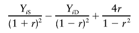on π_i- 1/2, with the intercept fixed at 0. This variant should be more robust to selected sampling. The t statistic for the test of the regression slope is

* * *

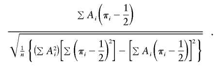The final four methods that we consider are score statistics based on the usual variance-components likelihood. Score statistics were proposed by Tang and Siegmund (2001), Wang and Huang (2002a), and Putter et al. (2002). The score statistics proposed in their articles are very similar to each other but have minor differences in how they parameterize the likelihood and how they alter the statistic to make it robust. Instead of considering precisely the statistics in the aforementioned articles, we take the Tang and Siegmund (2001) statistic as our starting point and propose four variations on possible ways to make it robust (or not). This allows us to draw careful conclusions about what kind of “robustification” is most desirable.

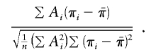
Asymptotic score statistic (SCORE1)

Tang and Siegmund (2001) derived a score statistic of the form

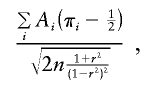where A_i is the same function as defined above for S&P2. The denominator of this statistic is based on asymptotic likelihood theory, so this version of the score statistic should not be robust to selected sampling or nonnormality.

Score statistic with partially empirical variance (SCORE2)

Tang and Siegmund (2001) proposed making their statistic robust by using the empirical variance of A_i in the denominator—that is,

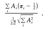The factor of is the SD of π when a perfectly informative marker is assumed. Thus, this version of the statistic should be robust to selected sampling but should yield a conservative test when there is imperfect IBD information.

Score statistic with fully empirical variance (SCORE3)

We propose that the best version of the score statistic should have the same form as SCORE2 but with the empirical SD of π in place of the factor of :

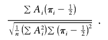This version should have correct type I error even with imperfect IBD information. A slightly different alternative would be to replace the  1/2 in the denominator of SCORE3 with , which would give very slightly higher type I error and slightly higher power than SCORE3 as we have defined it. Note that the S&P2 statistic, described above, is very similar to SCORE3 but has a cross-product term subtracted from the denominator. Again, that should yield a statistic with slightly higher type I error and power than SCORE3.

* * *

Score statistic with empirical mean and variance (SCORE4)

Both Wang and Huang (2002a) and Putter et al. (2002) proposed using in place of  1/2 in both the numerator and the denominator of the score statistic. When applied to our parameterization of the score statistic, that yields the expression

We emphasize that SCORE4 is not identical to either Wang and Huang's or Putter et al.’s statistics. Our SCORE4 should behave very similarly to SCORE3 in many cases, although it could have incorrect type I error in some situations, because correlations between and the π_i values are not accounted for in the denominator. That is, the denominator of SCORE4 is not actually the correct SD of the numerator—there are missing covariance terms. It would also be possible to consider a score statistic that incorporates the covariance terms, but we did not include such a statistic in our study.

For the following discussion, it is useful to classify our 12 statistics into three groups. The group I statistics (ORIGINAL.HE, TRAIT.SUM, and TRAIT.PRODUCT) use simple binary weights of the two regression slopes. These methods are all expected to have suboptimal power because of suboptimal weighting. The group II statistics (FORREST, V&H, and XU) use empirical variances to weight the two slopes. The group III statistics (S&P1, S&P2, SCORE1, SCORE2, SCORE3, and SCORE4) use the sibling trait correlation to achieve weighted statistics without calculation of empirical variance estimates.

All of the statistics that we consider, except ORIGINAL.HE, use an estimate of the trait mean, μ. Group III statistics additionally use estimates of the trait variance, σ², and sibling correlation, r. Sensitivity to these estimates may have an important effect on power.

Simulations

We studied the type I error and the power of each statistic under 11 trait models, which are described in table 1. All of the models are diallelic. Models 1–9 are standard mixture-of-normals models; the trait value is equal to the genotype mean plus a normally distributed “environmental” variance. There is an additional sibling correlation of 0.25 in each model, to account for environmental and polygenic components. The means and the variances were chosen to give each model a locus heritability of 0.2. Note the symmetry between certain pairs of models—between 1 and 7, between 2 and 9, between 3 and 8, and between 5 and 6. This symmetry means that type I error and power within each pair are identical for population samples, though not for selected samples. Models 1′ and 2′ were generated by simulating data under models 1 and 2, respectively, and then taking the signed square, , of each trait value. This yields overall trait distributions that are somewhat skewed and have high kurtosis. Models 3 and 8 also have skewness and kurtosis in the same range as models 1′ and 2′.

Table 1.

Genetic Models^[Note]

	Value for Model
Parameter	1	2	3	4	5	6	7	8	9	1′	2′
Model-defining:
Type of inheritancea	Add	Dom	Rec	Add	Dom	Rec	Add	Dom	Rec	Add	Dom
Locus heritability	.2	.2	.2	.2	.2	.2	.2	.2	.2	NA	NA
Allele frequency	.1	.1	.1	.5	.5	.5	.9	.9	.9	.1	.1
Trait means	−1, 0, 1	0, 1, 1	0, 0, 1	−1, 0, 1	0, 1, 1	0, 0, 1	−1, 0, 1	0, 1, 1	0, 0, 1	−1.6, 0, 1.6	0, 1.6, 1.6
Environmental SD	.849	.785	.199	1.414	.866	.866	.849	.199	.785	NA	NA
Environmental correlation	.25	.25	.25	.25	.25	.25	.25	.25	.25	NA	NA
Calculated:
Overall mean	−.8	.19	.01	.0	.75	.25	.8	.99	.81	−1.32	.295
Overall SD	.949	.877	.222	1.581	.968	.968	.949	.222	.877	2.047	1.393
Skewness	.168	.140	.880	.0971	−.0991	.102	−.168	−.880	−.140	−1.587	1.504
Kurtosis	.101	.0240	3.802	.0556	−.0714	−.031	.101	3.802	.0240	5.268	9.406
Overall correlation	.3	.3	.3	.3	.3	.3	.3	.3	.3	.25	.26

Note.— NA = not applicable.

^aAdd = additive; Dom = dominant; Rec = recessive.

Under each of the models, we simulated data for nuclear families with two children, and we ascertained families by two different methods. The first ascertainment scheme was simply population sampling—all families were used. The second scheme selected only those families in which at least one sibling fell in the top 10% of the trait distribution. We simulated data sets of 1,500 families for the population sampling and 500 families for the selected sampling. Figure 1 shows examples of simulated bivariate trait distributions for both sampling schemes under several of the models. To study type I error, we used 10,000 data sets, and, to study power, we used 1,000 data sets. The nominal type I error rate was set at 0.01. Marker data was simulated using eight equifrequent alleles, with the marker at recombination fraction (θ) 0 for the power study and at θ=0.5 for the type I error study. We also did power simulations at θ=0.05 for models 1 and 2 only.

Figure 1.

Scatterplots of population and selected samples from models 1, 2, and 1′

As discussed above (see the “Statistics Considered” subsection), most of the statistics require that some trait parameters (mean μ, variance σ², and sibling correlation r) be specified. In general, theory suggests that these should be population parameter values, even for selected samples. However, if one is using a selected sample, population parameter estimates may not be available. In that situation, parameter values must be guessed or adopted from previous studies in other populations. Using models 1 and 1′ only, we examined the robustness of the statistics to misspecification of parameters. We varied one parameter at a time while holding the other two parameters at the correct population values. Sibling correlation was set at 0.1 and 0.5, trait variance was set at values ranging from half the true value to twice the true value, and trait mean was set at the true mean ± 1 SD. We also did a limited number of studies in which two parameters at a time were misspecified. Finally, we checked the performance of the statistics when sample estimates of the parameters are used.

Results

Type I Error

Table 2 shows the SD and type I error of each statistic, based on the 10,000 simulated data sets of population samples.Table 3 shows the same information for the selected samples. All statistics had mean 0 for all models and for all sampling schemes. We show results for models 1–3, 1′, and 2′ only. Results for models 4–9 were very qualitatively similar to those for models 1–3. All of the statistics in these tables were computed with the known population values of the parameters (trait mean μ, variance σ², and sibling correlation r). The CIs for the estimated error rates in the tables are on the order of ±0.2% (i.e., an estimated error rate of 1.00% has a 95% CI of ∼0.80%–1.20%). We note first that the type I error and the SD for SCORE1 and SCORE2 are incorrect for essentially all models and sampling schemes. SCORE2 is always conservative (with low type I error) because of the perfect-IBD assumption; SCORE1 is highly variable, presumably because the asymptotic-normality assumption underlying it is inappropriate for many of these trait distributions. V&H and FORREST have incorrect type I error for the most non-Gaussian models (3, 1′, and 2′) under population sampling and for all models under selected sampling; this is due to the omission of the covariance term in the weighting. Finally, SCORE4 has low type I error for some models under selected sampling, because of the missing covariance in the denominator of the statistic; the size of the covariance term depends heavily on the A_i values, and, for some models and sampling schemes, it can be quite large. As predicted, S&P2 and SCORE3 are very similar, with S&P2 having a slightly higher type I error rate for most models. We did limited experiments (results not shown) with a version of SCORE3 that replaces  1/2 in the denominator with (see the “Methods” section) and found that it has type I error rates that are just about identical to those of S&P2.

Table 2.

SD and Type I Error for Population Samples

	SD and Type I Error under Model
	1		2		3		1′		2′
Statistic	SD	Error(%)	SD	Error(%)	SD	Error(%)	SD	Error(%)	SD	Error(%)
Group I:
ORIGINAL.HE	1.01	1.17	1.01	1.07	.99	1.00	1.00	1.02	1.00	1.12
TRAIT.SUM	1.01	1.16	.99	1.03	.99	.94	1.01	1.05	1.00	.84
TRAIT.PRODUCT	1.02	1.16	1.00	1.00	.99	.88	1.00	1.03	1.00	.86
Group II:
XU	1.01	1.12	1.01	1.03	.99	.89	1.00	.89	.99	.94
V&H	1.01	1.12	1.01	.99	.85	.26	.72	.12	.63	.01
FORREST	1.01	1.12	1.01	1.02	.86	.34	.75	.15	.69	.04
Group III:
S&P1	1.01	1.13	1.01	1.05	.99	.94	1.00	1.01	1.00	.93
S&P2	1.02	1.12	1.01	1.04	.99	.93	1.00	1.06	1.00	.93
SCORE1	.96	.70	1.01	.76	1.29	3.53	1.10	1.87	3.26	23.00
SCORE2	.94	.65	1.01	.63	.92	.58	.92	.55	.93	.50
SCORE3	1.01	1.10	1.01	1.00	.99	.92	.99	1.06	1.00	.90
SCORE4	1.01	1.12	1.01	1.03	.99	.94	1.00	.99	.98	.84

Table 3.

SD and Type I Error for Selected Samples

	SD and Type I Error under Model
	1		2		3		1′		2′
Statistic	SD	Error(%)	SD	Error(%)	SD	Error(%)	SD	Error(%)	SD	Error(%)
Group I:
ORIGINAL.HE	1.00	1.00	1.00	.90	1.01	1.18	1.01	.97	1.00	.75
TRAIT.SUM	1.00	.89	1.00	1.10	.99	.79	1.02	1.00	1.00	1.03
TRAIT.PRODUCT	1.00	.90	1.01	1.00	.99	.84	1.02	1.00	1.00	.98
Group II:
XU	1.00	1.01	1.00	.97	1.00	1.05	1.01	.93	.99	.98
V&H	1.11	1.66	1.05	1.20	.90	.55	.87	.35	.75	.08
FORREST	1.13	1.83	1.15	2.10	.91	.60	.91	.41	.79	.13
Group III:
S&P1	1.00	.94	1.00	1.00	1.00	1.03	1.01	.93	.99	.84
S&P2	1.00	1.04	1.01	1.20	1.00	1.05	1.02	1.10	.99	.85
SCORE1	1.62	7.21	1.90	11.00	2.75	19.48	3.25	24.00	7.63	37.54
SCORE2	.93	.64	.93	.76	.92	.68	.94	.63	.92	.50
SCORE3	1.00	.98	1.00	1.20	.99	1.01	1.01	1.10	.99	.80
SCORE4	.99	.87	.86	.34	.98	.88	.83	.17	.93	.48

Power

Table 4 gives the power for all models for the population samples, and table 5 gives the power for the selected samples. Again, all of the statistics in these tables were computed with the known population values of the parameters. To make comparisons simpler, we omitted from the power tables the statistics that did not have correct type I error. The number of replicates for the power study was 1,000, so the 95% CI for a power estimate of 50% is ∼47%–53%. The general qualitative results are quite similar for the two sampling schemes. The group I statistics have lower power than the group II and group III statistics in almost all cases. This is attributable to the suboptimal weighting of the sum and difference regression slopes in the group I statistics. All of the group II and group III statistics have essentially identical power, with the exception that XU has noticeably higher power for models 1′ and 2′. We did limited experiments (results not shown) with a version of SCORE3 that replaces  1/2 in the denominator with (see the “Methods” section) and found, as predicted, that it has power rates that are just about identical to those of S&P2. We also did power simulations at θ=0.05 for models 1 and 2 only (results not shown); although the overall power is lower than at θ=0, the relative power of the different statistics is unchanged.

Table 4.

Power for Population Samples

	Power under Model
Statistic	1	2	3	4	5	6	7	8	9	1′	2′
Group I:
ORIGINAL.HE	.61	.60	.23	.59	.57	.57	.58	.22	.56	.09	.15
TRAIT.SUM	.15	.19	.07	.19	.19	.20	.16	.07	.16	.03	.04
TRAIT.PRODUCT	.53	.55	.27	.54	.55	.57	.53	.25	.51	.15	.36
Group II:
XU	.71	.73	.39	.72	.72	.70	.71	.37	.69	.21	.54
Group III:
S&P1	.71	.73	.42	.72	.71	.70	.71	.40	.69	.21	.44
S&P2	.71	.73	.41	.72	.71	.70	.71	.40	.69	.21	.43
SCORE3	.71	.73	.41	.72	.71	.69	.71	.40	.69	.21	.43

Table 5.

Power for Selected Samples

	Power under Model
Statistic	1	2	3	4	5	6	7	8	9	1′	2′
Group I:
ORIGINAL.HE	.84	.82	.72	.58	.33	.75	.29	.04	.28	.39	.23
TRAIT.SUM	.61	.66	.24	.35	.15	.55	.10	.01	.12	.17	.18
TRAIT.PRODUCT	.85	.87	.76	.57	.31	.80	.23	.03	.23	.70	.62
Group II:
XU	.89	.88	.92	.64	.36	.83	.29	.02	.31	.77	.75
Group III:
S&P1	.90	.89	.93	.65	.36	.84	.28	.03	.31	.73	.65
S&P2	.91	.91	.97	.66	.37	.86	.28	.03	.31	.69	.68
SCORE3	.91	.91	.94	.65	.37	.85	.28	.03	.30	.69	.67

Sensitivity

All of the statistics except ORIGINAL.HE use estimates of the mean (μ) parameter. In addition, all of the group III statistics involve the sibling correlation (r) and variance (σ²) parameters. To assess the robustness of the statistics to misspecification of the trait parameters, we first tried using the sample parameter values for each data set, rather than the known population values. The use of sample parameter values does not change the type I error (results not shown). For population samples, as one would expect, the use of sample parameter estimates also has no effect on power. For selected samples, there is a drastic reduction in power for all statistics and all models (results not shown). This is not surprising, since sample estimates calculated from selected samples are generally quite far off from the correct population values.

We next investigated the effect of misspecifying one parameter at a time. For each run, we set two of the parameters to the population values and set the third parameter to an arbitrary “wrong guess” (see the “Methods” section). We performed these sensitivity studies for models 1 and 1′ only. Tables 6–9 give the power results (type I error was not sensitive to parameter misspecification for any of the statistics). For each table, we generated a single set of 1,000 data sets and analyzed them under different assumed parameter values. Table 6 shows power results for model 1 with population sampling, table 7 shows the results for model 1′ with population sampling, and tables 8 and 9 give the results for selected sampling.

Table 6.

Power for Population Samples—Sensitivity Analyses under Model 1

	Power, Assuming
Statistic	r=.1	r=.5	μ=-1.75	μ=.15	σ2=.45	σ2=1.8	Correct PopulationParameter Values
Group I:
ORIGINAL.HE	.61	.61	.61	.61	.61	.61	.61
TRAIT.SUM	.15	.15	.04	.05	.15	.15	.15
TRAIT.PRODUCT	.53	.53	.15	.17	.53	.53	.53
Group II
XU	.71	.71	.65	.63	.71	.71	.71
Group III
S&P1	.63	.69	.49	.47	.71	.71	.71
S&P2	.61	.65	.41	.42	.71	.67	.71
SCORE3	.61	.65	.41	.42	.71	.67	.71

Table 7.

Power for Population Samples—Sensitivity Analyses under Model 1′

	Power, Assuming
Statistic	r=.1	r=.5	μ=-3.37	μ=.73	σ2=2.095	σ2=8.38	Correct PopulationParameter Values
Group I:
ORIGINAL.HE	.09	.09	.09	.09	.09	.09	.09
TRAIT.SUM	.03	.03	.04	.02	.03	.03	.03
TRAIT.PRODUCT	.15	.15	.09	.05	.15	.15	.15
Group II:
XU	.21	.21	.11	.18	.21	.21	.21
Group III:
S&P1	.20	.13	.12	.15	.21	.21	.21
S&P2	.19	.12	.11	.13	.20	.20	.21
SCORE3	.19	.12	.11	.12	.20	.20	.21

Table 8.

Power for Selected Samples—Sensitivity Analyses under Model 1

	Power, Assuming
Statistic	r=.1	r=.5	μ=-1.75	μ=.15	σ2=.45	σ2=1.8	Correct PopulationParameter Values
Group I:
ORIGINAL.HE	.84	.84	.84	.84	.84	.84	.84
TRAIT.SUM	.61	.61	.64	.14	.61	.61	.61
TRAIT.PRODUCT	.85	.85	.80	.91	.85	.85	.85
Group II:
XU	.89	.89	.79	.78	.89	.89	.89
Group III:
S&P1	.88	.88	.88	.89	.90	.90	.90
S&P2	.83	.87	.63	.85	.91	.90	.91
SCORE3	.82	.87	.62	.85	.91	.89	.91

Table 9.

Power for Selected Samples—Sensitivity Analyses under Model 1′

	Power, Assuming
Statistic	r=.1	r=.5	μ=-3.37	μ=.73	σ2=2.095	σ2=8.38	Correct PopulationParameter Values
Group I:
ORIGINAL.HE	.39	.39	.39	.39	.39	.39	.39
TRAIT.SUM	.17	.17	.32	.00	.17	.17	.17
TRAIT.PRODUCT	.70	.70	.59	.31	.70	.70	.70
Group II:
XU	.77	.77	.70	.27	.77	.77	.77
Group III:
S&P1	.76	.54	.74	.50	.73	.73	.73
S&P2	.63	.58	.21	.52	.73	.58	.69
SCORE3	.63	.57	.21	.52	.72	.58	.69

For the population samples (tables 6 and 7), misspecification of the variance has very little effect. Misspecification of the correlation does reduce power slightly for the group III statistics. Misspecification of the mean substantially reduces the power of the group III statistics and reduces the power of XU slightly. ORIGINAL.HE, which does not depend on the mean, has roughly equivalent power to XU when the mean is misspecified for model 1 but not for model 1′. Overall, XU seems to be the statistic with the best power in the context of parameter misspecification.

For the selected samples from model 1 (table 8), misspecification of the variance again has very little effect. Misspecification of the correlation slightly decreases the power of the group III statistics. Misspecification of the mean causes moderate decreases in power, and S&P1 seems to be the most resistant to this effect. ORIGINAL.HE and TRAIT.PRODUCT perform just about as well as the group II and group III statistics do when the parameters are misspecified. Overall, in table 8, S&P1, TRAIT.PRODUCT, and ORIGINAL.HE appear to be the most robust statistics. For selected samples from model 1′ (table 9), we obtain fairly similar results, and S&P1 again appears to have the most robust power. For this model, however, ORIGINAL.HE and TRAIT.PRODUCT are not as powerful. Note that misspecification actually increases the power in some cases, presumably because the population trait parameters are optimal only under normality assumptions.

We did a limited study of the effects of misspecifying two parameters at a time. Detailed results are not shown, but the general qualitative result was that power was driven by how badly the mean was misspecified. This is consistent with the “one parameter wrong” runs described above, in which the mean had, by far, the greatest effect on power.

Discussion

We have performed the most comprehensive comparison to date of sibling-pair QTL-mapping statistics. We used simulation to evaluate the type I error and the power of 12 different statistics under both population sampling and selected sampling. Seven of the statistics (ORIGINAL.HE, TRAIT.SUM, TRAIT.PRODUCT, XU, S&P1, S&P2, and SCORE3) have consistently correct type I error over all the models and the sampling schemes that we considered. If one considers the results for perfectly known trait parameters only, then the statistics with the highest power are XU, S&P1, S&P2, and SCORE3; they are just about equivalent, except that XU has higher power for the nonnormal trait models that we studied. This suggests that any of those statistics would be appropriate for most studies, with a possible preference for XU, depending on the trait distribution. However, when the effect of parameter misspecification is taken into account, the picture changes somewhat. For population samples, XU appears to have the most robust power, but, if one has a population sample, then one also has decent estimates of the population parameters. Parameter misspecification is a much more important issue for selected samples, and S&P1 seems most robust in that case.

Our results are basically consistent with those of previous studies. The finding that the group I statistics are not as powerful as the group II statistics was demonstrated previously by a number of different authors, including Xu et al. (2000), Forrest (2001), and Visscher and Hopper (2001). Neither Forrest (2001) nor Visscher and Hopper (2001) observed incorrect type I error for their methods, but they looked only at population samples from a limited number of distributions. The sensitivity of TRAIT.PRODUCT to misspecification of the mean was examined by Palmer et al. (2000) and Zhang et al. (2002). The approximate equivalence, based on analytical arguments, of XU, S&P1, and S&P2 was noted by Sham and Purcell (2001). The similarity (again based on analytical arguments) between S&P2 and the score statistics was noted by Feingold (2001).

There are, of course, limitations to our study in the types of samples considered, in the models considered, and in the statistics considered. In terms of the types of samples, the most important limitation is that we considered sibling pairs only. Real studies generally include larger sibships as well. Of the more powerful statistics considered, XU and the score statistics generalize to larger sibships, whereas S&P1 and S&P2 do not. It is possible that the different methods for the handling of larger sibships result in substantial power differences, so further study of these methods is very important. A method that was developed specifically for extended pedigrees is the regression-based method of Sham et al. (2002), which we discuss in further detail below.

An additional limitation in the types of samples considered is that we studied one-tailed sampling (one sibling in the top 10%), ignoring two-tailed sampling (one sibling in the top 10% or in the bottom 10%). We expect that the statistical-performance results for one tail would generally hold for two tails. Statistics with incorrect type I error for one-tailed sampling will likely be incorrect also for two-tailed sampling. The group of statistics with equally high power for one-tailed sampling is likely to also have the highest power for two-tailed sampling. The companion article (Szatkiewicz et al. 2003 [in this issue]) considers discordant pairs (one sibling in the top 10% and one sibling in the bottom 10%); for that type of sampling, the results are quite different from those presented in the present article.

We considered only large sample sizes (large numbers of sibling pairs). We assume that studies with small samples are fairly unusual.

There are also some limitations to the models that we studied. All of our models used an environmental/polygenic sibling correlation of 0.25. This should not affect the relative power of the group II and group III statistics. It does affect the relative power of the group I statistics, but, since this is well documented (Palmer et al. 2000; Forrest 2001), we did not explore it in detail here. It does mean that the relative power of ORIGINAL.HE and TRAIT.PRODUCT that we observed should not be taken as a general rule. In general, the greater the correlation, the better ORIGINAL.HE performs in comparison to TRAIT.PRODUCT. We do see a need for further exploration of a wide variety of nonnormal models. The fact that our results for models 1′ and 2′ were significantly different from our results for mixture-of-normals models indicates the need for further work, preferably with careful consideration given to what types of models are realistic.

In the literature, there are several important statistics that we did not include in our study. We did not consider variance components, because our main focus was on selected sampling, and it is well documented that variance-components analysis has incorrect type I error in such cases (e.g., see Allison et al. 1999; Sham et al. 2000). There are, however, various robust versions of variance-components analysis (for review, see Feingold 2001) that could be more carefully compared to the methods discussed here. We also did not consider the precise score statistics proposed by Wang and Huang (2002a) and Putter et al. (2002). Given that SCORE3 performs very well, further study of other score-statistic variations might be useful. The statistic proposed by Sham et al. (2002), mentioned above, was developed specifically to be a robust statistic for extended pedigrees. It regresses IBD on trait values—the opposite of the statistics discussed in the present article. For sibling pairs, it has exactly the same form as SCORE2 and SCORE3 but with the variance of π in the denominator estimated differently.

Finally, a few potentially useful variations on the statistics that we considered are not yet in the literature. One could use any of the statistics here with the parameter estimates chosen (on the basis of the data) to maximize the value of the statistic. This is particularly appealing as a way to deal with the sensitivity to the mean. Similarly, one could use a statistic that weights the squared-sum and squared-difference regressions, such as XU, but with the weights maximized for the particular data set. Either of these approaches would entail the loss of a degree of freedom to properly adjust for the maximization; we suspect that, as a result, there would not be a useful power gain, but further study is warranted.

References

- Allison DB, Fernández JR, Heo M, Beasley TM (2000) Testing the robustness of the new Haseman-Elston quantitative-trait loci–mapping procedure. Am J Hum Genet 67:249–252 [DOI] [PMC free article] [PubMed] [Google Scholar]
- Allison DB, Neale MC, Zannolli R, Schork NJ, Amos CI, Blangero J (1999) Testing the robustness of the likelihood-ratio test in a variance-component quantitative-trait loci–mapping procedure. Am J Hum Genet 65:531–544 [DOI] [PMC free article] [PubMed] [Google Scholar]
- Almasy L, Blangero J (1998) Multipoint quantitative-trait linkage analysis in general pedigrees. Am J Hum Genet 62:1198–1211 [DOI] [PMC free article] [PubMed] [Google Scholar]
- Amos CI (1994) Robust variance-components approach for assessing genetic linkage in pedigrees. Am J Hum Genet 54:535–543 [PMC free article] [PubMed] [Google Scholar]
- Drigalenko E (1998) How sib pairs reveal linkage. Am J Hum Genet 63:1242–1245 [PMC free article] [PubMed] [Google Scholar]
- Elston RC, Buxbaum S, Jacobs KB, Olson JM (2000) Haseman and Elston revisited. Genet Epidemiol 19:1–17 [DOI] [PubMed] [Google Scholar]
- Feingold E (2001) Methods for linkage analysis of quantitative trait loci in humans. Theor Popul Biol 60:167–180 [DOI] [PubMed] [Google Scholar]
- ——— (2002) Regression-based quantitative-trait–locus mapping in the 21st century. Am J Hum Genet 71:217–222 [DOI] [PMC free article] [PubMed] [Google Scholar]
- Forrest W (2001) Weighting improves the “new Haseman-Elston” method. Hum Hered 52:47–54 [DOI] [PubMed] [Google Scholar]
- Ghosh S, Reich T (2002) Integrating sibship data for mapping quantitative trait loci. Ann Hum Genet 66:169–182 [DOI] [PubMed] [Google Scholar]
- Goldstein DR, Dudoit S, Speed TP (2001) Power and robustness of a score test for linkage analysis of quantitative traits using identity by descent data on sib pairs. Genet Epidemiol 20:415–431 [DOI] [PubMed] [Google Scholar]
- Haseman JK, Elston RC (1972) The investigation of linkage between a quantitative trait and a marker locus. Behav Genet 2:3–19 [DOI] [PubMed] [Google Scholar]
- Palmer LJ, Jacobs KB, Elston RC (2000) Haseman and Elston revisited: the effects of ascertainment and residual familial correlations on the power to detect linkage. Genet Epidemiol 19:456–460 [DOI] [PubMed] [Google Scholar]
- Putter H, Sandkuijl LA, van Houwelingen JC (2002) Score test for detecting linkage to quantitative traits. Genet Epidemiol 22:345–335 [DOI] [PubMed] [Google Scholar]
- Sham PC, Purcell S (2001) Equivalence between Haseman-Elston and variance-components linkage analyses for sib pairs. Am J Hum Genet 68:1527–1532 [DOI] [PMC free article] [PubMed] [Google Scholar]
- Sham PC, Purcell S, Cherny SS, Abecasis GR (2002) Powerful regression-based quantitative-trait linkage analysis of general pedigrees. Am J Hum Genet 71:238–253 [DOI] [PMC free article] [PubMed] [Google Scholar]
- Szatkiewicz JP, T.Cuenco K, Feingold E (2003) Recent advances in human quantitative-trait–locus mapping—comparison of methods for discordant sibling pairs. 73:874–885 (in this issue) [DOI] [PMC free article] [PubMed] [Google Scholar]
- Tang H-K, Siegmund D (2001) Mapping quantitative trait loci in oligogenic models. Biostatistics 2:147–162 [DOI] [PubMed] [Google Scholar]
- ——— (2002) Mapping multiple genes for quantitative or complex traits. Genet Epidemiol 22:313–327 [DOI] [PubMed] [Google Scholar]
- Visscher PM, Hopper JL (2001) Power of regression and maximum likelihood methods to map QTL from sib-pair and DZ twin data. Ann Hum Genet 65:583–601 [DOI] [PubMed] [Google Scholar]
- Wang K (2002) Efficient score statistics for mapping quantitative trait loci with extended pedigrees. Hum Hered 54:57–68 [DOI] [PubMed] [Google Scholar]
- Wang K, Huang J (2002a) A score-statistic approach for the mapping of quantitative–trait loci with sibships of arbitrary size. Am J Hum Genet 70:412–424 [DOI] [PMC free article] [PubMed] [Google Scholar]
- ——— (2002b) Score test for mapping quantitative-trait loci with sibships of arbitrary size when the dominance effect is not negligible. Genet Epidemiol 23:398–412 [DOI] [PubMed] [Google Scholar]
- Xu X, Weiss S, Xu X, Wei LJ (2000) A unified Haseman-Elston method for testing linkage with quantitative traits. Am J Hum Genet 67:1025–1028 [DOI] [PMC free article] [PubMed] [Google Scholar]
- Zhang W, Collins A, Lonjou C, Morton NE (2002) A linkage tournament: affection status, parametric analysis, multivariate traits, and enhancements to variance components and relative pairs. Ann Hum Genet 66:87–98 [DOI] [PubMed] [Google Scholar]
- Zhang W, Tapper W, Collins A, Jacobs KB, Elston RC (2001) A tournament of linkage tests in complex inheritance. Hum Hered 52:140–148 [DOI] [PubMed] [Google Scholar]