Positional Cloning by Linkage Disequilibrium

Abstract

Recently, metric linkage disequilibrium (LD) maps that assign an LD unit (LDU) location for each marker have been developed (Maniatis et al. 2002). Here we present a multiple pairwise method for positional cloning by LD within a composite likelihood framework and investigate the operating characteristics of maps in physical units (kb) and LDU for two bodies of data (Daly et al. 2001; Jeffreys et al. 2001) on which current ideas of blocks are based. False-negative indications of a disease locus (type II error) were examined by selecting one single-nucleotide polymorphism (SNP) at a time as causal and taking its allelic count (0, 1, or 2, for the three genotypes) as a pseudophenotype, Y. By use of regression and correlation, association between every pseudophenotype and the allelic count of each SNP locus (X) was based on an adaptation of the Malecot model, which includes a parameter for location of the putative gene. By expressing locations in kb or LDU, greater power for localization was observed when the LDU map was fitted. The efficiency of the kb map, relative to the LDU map, to describe LD varied from a maximum of 0.87 to a minimum of 0.36, with a mean of 0.62. False-positive indications of a disease locus (type I error) were examined by simulating an unlinked causal SNP and the allele count was used as a pseudophenotype. The type I error was in good agreement with Wald’s likelihood theorem for both metrics and all models that were tested. Unlike tests that select only the most significant marker, haplotype, or haploset, these methods are robust to large numbers of markers in a candidate region. Contrary to predictions from tagging SNPs that retain haplotype diversity, the sample with smaller size but greater SNP density gave less error. The locations of causal SNPs were estimated with the same precision in blocks and steps, suggesting that block definition may be less useful than anticipated for mapping a causal SNP. These results provide a guide to efficient positional cloning by SNPs and a benchmark against which the power of positional cloning by haplotype-based alternatives may be measured.

Introduction

Positional cloning aims to localize determinants of disease susceptibility in the DNA sequence prior to determining their function. Linkage mapping is routinely used to locate major genes, which are relatively rare but have a large phenotypic effect. However, this method has had limited success when applied to mapping oligogenes, which are more common but have a smaller effect. Even with major alleles, the error in localization may be appreciable. Efforts to map oligogenes are concerned with exploiting allelic association (also called “linkage disequilibrium” [LD]) between markers and putative disease-predisposing loci. The first applications were to major loci that could be assigned to haplotypes by family study (Kerem et al. 1989; Devlin and Risch 1995; Terwilliger 1995). These and other studies have provided the foundation for the application of LD mapping for postional cloning of common diseases in complex inheritance. This enthusiasm has been escalated by the discovery of millions of SNPs (Kruglyak and Nickerson 2001), most of which cannot be subject to measurable selection (Kimura 1986). The utility of SNPs for association studies is now well established, and recent technological advances have made it feasible to identify and sequence a large number of SNPs. Current estimates suggest that the human genome may have as many as 15 million such markers (Botstein and Risch 2003). Among this vast number of polymorphisms is a much smaller number that have a significant role in common diseases. LD analysis offers the prospect of high-resolution mapping because it can provide sufficient information to narrow the region and refine the location of the disease genes, particularly when SNPs are densely typed in a candidate region.

LD is present when recombination between alleles at small distance is infrequent. There is much variation in the extent of LD in different chromosome regions, reflecting the nonuniform distribution of recombination events. There are many evolutionary and other confounding factors that influence the extent of LD, such as genetic drift, mutation, and selection, but recombination appears to dominate the pattern of LD. Several studies have demonstrated that the pattern of LD is highly structured into blocks of low haplotype diversity with strong LD (Daly et al. 2001) and regions of low LD, which correspond to recombination hotspots (Jeffreys et al. 2001). There has been much emphasis on determining the haplotype-block structure of the human genome (Daly et al. 2001). However, the utility of haplotype-block identification for disease-gene localization remains uncertain. Maniatis et al. (2002) provided an alternative approach, which develops a metric map in LD units (LDUs) to describe the underlying pattern of LD. On the basis of the Malecot equation, which was adopted to describe the decline of LD with distance (Collins and Morton 1998; Collins et al. 1999), LDU maps discriminate blocks of conserved LD with additive distances and locations monotonic with physical (kb) maps. LDU maps are analogous to the genetic linkage map but with much higher resolution. Their properties have been studied, and there is clear evidence that a map in LDU has a smaller empirical error variance than a map in kb (Zhang et al. 2002). The first metric LD map of human chromosome 22 has also recently been constructed, and this shows good correspondence with the deCODE linkage map (Kong et al. 2002), despite the evolutionary error variance in LDU maps and low resolution of the linkage map (Tapper et al. 2003). Unlike haplotype blocks, LDU maps provide a scale on which to distribute SNPs optimally and to localize disease genes within candidate regions. This is analogous to creating a high-resolution linkage map for positional cloning of major genes by LD (Collins and Morton 1998; Lonjou et al. 1998a, 1998b; Morton and Collins 1998). Nevertheless, we have no information about the operating characteristics and the optimal use of an LD map for positional cloning. Here we present a multiple pairwise method in which we use composite likelihood to investigate positional cloning by LD. One of the key objectives is to assess the power and precision for localization of causal polymorphisms achieved by using an LDU map, compared with a map in kb, for two extensive bodies of data on which current ideas of blocks and steps are based.

Material and Methods

LD Maps

The first data set, from 50 unrelated North European males, was presented by Jeffreys et al. (2001) and consists of 296 SNPs typed in a 216-kb segment of the class II region of the major histocompatibility complex in 6p21.3. Their high-resolution LD analysis showed extended domains of strong association, separated by peaks of LD breakdown, which correspond precisely to meiotic crossover hotspots on the basis of sperm typing. The second data set, presented by Daly et al. (2001), consists of 103 SNPs typed in a 617-kb segment on chromosome 5q31. By latent variable analysis, Daly et al. delimited 11 blocks in 129 parent-child trios from a European-derived population. We sampled only parents for diplotypes (phase-unknown genotypes) from these data. Also, we followed the example of Daly et al. and rejected SNPs with minor allele frequencies <0.05, reducing the sample of Jeffreys et al. to 248 SNPs. Although the two samples are comparable in these respects, they differ in sample size, marker density, and steepness of steps (fig. 1).

Figure 1.

Graphs of the LD maps for the data sets from Daly et al. (2001) (A) and Jeffreys et al. (2001) (B). For comparison between the LDU maps and the block-step structure of A and B, see Zhang et al. (2002).

Every marker in the data was assigned two locations, one in kb and the other in LDU. The LD maps developed by Maniatis et al. (2002) assign locations to markers in LDU, which describe the underlying structure of LD in the form of a metric map and thus avoid arbitrary block definitions. The theoretical framework for constructing LD maps is based on the Malecot equation, which describes association probability (ρ) between any pair of SNPs as ρ=(1-L)Me^-ɛd+L, where ρ is the predicted association with observed estimate . The absolute value of D is the covariance in a 2 × 2 haplotype table, with minor allele frequencies Q⩽R, 1-Q. This can always be satisfied by interchanging the columns and rows of the 2 × 2 matrix; thus, Q (frequency of the putatively younger allele) is <0.5, but R can exceed 0.5. The metric is unique in providing evolutionary theory to which other metrics fit less well (Morton et al. 2001; Shete 2003). With association declining exponentially with distance, the intercept M determines maximum association at zero distance and is a parameter with evolutionary interpretation, since it reflects the association at the last major bottleneck. Values of M≪1 suggest polyphyletic origin of haplotypes. The horizontal asymptote L>0 is the association at large distance, and hence the model corrects for the inflated associations resulting from small sample size. The parameter ɛ is the exponential decline of disequilibrium ρ with distance d. The LDU map method estimates ɛ in each map interval and uses this to construct an LD scale. A map distance in LDUs is ɛ_id_i for the ith interval with a region having LDUs (Maniatis et al. 2002). The mean ɛ for the region is , and its inverse is termed the “swept radius 1/ɛ,” which gives the extent of useful LD, with 0<ɛ<1 on the kb scale and ɛ=1 for a standard LD map. One of the elegant properties of the model is that recombination affects only ɛ but not M, whereas mutation and drift systematically affect only M. The asymptote L can be estimated or predicted (L_p) from the information about , which is proportional to sample size (Morton et al. 2001; Maniatis et al. 2002). In small sequences (for example, the sample of Jeffreys et al. spans only 216 kb), the predicted value gives a more reliable LD map than the direct estimate, which is distorted by deviations of the block structure from the Malecot model (Zhang et al. 2002). Regions with extensive disequilibrium have few LDU and low recombination. LDU reveal a pattern of steps and plateaus. Plateaus (i.e., ɛ_i=0) correspond to blocks of low haplotype diversity, whereas steps (i.e., ɛ_i>0) correspond to recombination events, the magnitude of which reflects recombination intensity. Blocks and steps can also be graphically presented by plotting LDU maps against kb locations for both data sets, as is shown in figure 1. A value of ɛ_id_i > 2 or 3 indicates a “hole” within which further SNP typing is required for efficient positional cloning (Tapper et al. 2003). Zhang et al. (2002) constructed LDU maps for the aforementioned data sets. They found a remarkable agreement between LDU steps and sites of meiotic recombination in data presented by Jeffreys et al. (2001), which is informative for crossing over and is in good agreement with the method presented by Daly et al. (2001) that defines blocks without assigning an LD location to each marker. The LDU map methodology has been implemented in the program LDMAP.

Positional Cloning

The main objective of LD mapping is to facilitate positional cloning. The association metric has been shown to be optimal for describing patterns of LD (Morton et al. 2001). However, cannot be obtained for association between a trait and a marker SNP, solely because the frequency Q of the putative disease allele is unknown. The metric requires the frequency of the causal SNP (Q) to be less than or equal to the frequency of the positively associated marker allele (R). This constraint can be met for major genes in which case and control haplotypes can be distinguished through family study. Therefore, is useful for marker-by-marker association, as exploited in constructing LD maps and for major genes but not for localizing oligogenes in complex inheritance. Having used to create an LD map, we must use other metrics for positional cloning of oligogenes.

Association can instead be represented by regression (b) or correlation (r) coefficients between the phenotype (Y) and the genotype (X) of each SNP locus. There is a plethora of LD metrics, from which Devlin and Risch (1995) considered a subset applicable to case-control studies, and of these regression and correlation have a strong statistical basis. The coefficient b, with marker allele count X as the independent variable, can be adapted to random samples, case-control studies, and families (Abecasis et al. 2000). The distribution of the independent variable is not specified, but deviations from the regression line are assumed to be normal and homoscedastic, as they might be if the dependent variable Y were quantitative. The r coefficient has a known normal distribution when both variables are normal and linearly related, but under the null hypothesis (r=0) the distribution is not normal.

We have developed an assay that is based on n+1 diallelic markers, one of which is designated as causal by taking its allelic count as a pseudophenotype Y=0, 1, or 2 for genotypes PP, PP′, and P′P′, respectively. The ith predictive SNP is assigned its allelic count X_i=0, 1, or 2 for genotypes G_iG_i, G_iG_i′, and G_i′G_i′, respectively (i=1, …, n). The type II error for the two metrics and maps is determined by selecting one among n+1 linked markers as causal (pseudophenotype) and repeating this for all markers. The number of tests performed is equal to the number of SNPs. Therefore, false-negative indications of a disease locus were investigated under the hypothesis that the pseudophenotype is not in the region in question. All analyses considered here are based on the additive model, with the three genotypes of each SNP as the independent variables. This schema, however, may be modified to include dominance or recessive effects. The metrics can easily accommodate a continuous phenotype and case-control samples (Collins and Morton 1998). Haplotypes can also be used, but the optimal method is yet to be developed.

Association of the pseudophenotype with each SNP in the map was modeled by a multiple pairwise method. An adaptation of the Malecot model to include a parameter for location of the putative gene was employed in a composite likelihood framework. We constructed the composite likelihood by the sum of marginal log likelihood, , where is an observed association metric ( or ) at the ith marker SNP with information K. The expected value of ψ_i (b_i or r_i) is obtained from the Malecot equation, ψ_i=(1-L)Me^-ɛΔ(S_i-S)+L, where S_i is the marker location in either kb or LDU of the ith predictive SNP with allelic count X_i. S, on the other hand, is the unknown parameter in the model and provides the estimated causal location. The Kronecker Δ is used solely for map direction and takes the value 1 if S_i>S and −1 otherwise (Collins and Morton 1998). When using the metrics and , the parameter M in the Malecot model no longer has an evolutionary interpretation, since it is not based on the allele-frequency–dependent metric . Instead, it represents the degree of association between the phenotype and the marker SNPs. 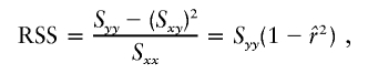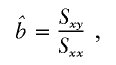For metric , the parameter M is constrained to the 0–1 range, but it may exceed 1 for when the phenotype is a quantitative trait and not an allele count, as in the present analysis. The residual variance is V_ψ=-2lnlk/(n-k), where n is the number of markers and k is the number of parameters estimated in the Malecot model (Collins and Morton 1998). The relevant formulae for regression of Y on X in a random sample of n diplotypes are as follows:

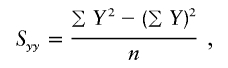residual sum of squares

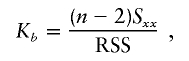
where K_ψi is the information about or and χ²₁=ψ²K_ψ asymptotically. Taking the absolute value of or is equivalent to reversing the allelic count of the three genotypes (i.e., X_i=0, 1, or 2 for genotypes G_i′G_i′, G_iG_i′, and G_iG_i, respectively). Because of the singularity of K_ψ, with the few cases where r approaches 1, we impose max K_r=(n-2)/(1-.99²) and max K_b=[(n-2)(S_xx)]/[(S_yy)(1-.99²)]. A marker with S_xx=0 is omitted as uninformative.

The use of composite likelihood raises legitimate questions about the reliability of significance tests (Devlin et al. 1996). To address these concerns, we examined the type I error by simulating under panmixia an unlinked SNP (nonsyntenic) from a trinomial distribution in Hardy-Weinberg proportions for a gene frequency of 0.5. Therefore, false-positive indications of a disease locus were investigated under the hypothesis that the simulated SNP is not in the region in question. With real data, the disease phenotype would be shuffled instead of simulated for the type I error test. We also established that the choice of gene frequency (0.05–0.5) was not critical (results not shown).

Positional cloning by LD focuses on refining the resolution of a candidate region. Testing for the potential existence of a causal SNP within a region in question requires hierarchical modeling of LD. This is accomplished by comparing models A–D. The baseline is model A, in which none of the parameters is estimated, so M=0 and ψ_i=L_p. Thus, model A is taken as the null hypothesis H₀ where there is no association between the pseudophenotype and marker SNPs. Model B is similar to model A, except that L is estimated, so any significant increase in L above the predicted asymptote provides evidence for a disease determinant within a region of interest without precise localization (ψ_i=L). Models A and B test for a candidate region but do not estimate a causal location. Models C and D are like models A and B regarding L, respectively, but parameters M and S are estimated. Therefore, the contrasts A-C and A-D test for a disease determinant at location S. The D model is the most complex alternative hypothesis, since it estimates all three parameters: L, M, and S. For all models, the ɛ parameter was fixed to 1 for the LDU map and to the mean value of ɛ for the kb map, obtained from the pairwise marker-by-marker association analysis for the whole region. Any attempt to estimate all four parameters gives incredibly high estimates of ɛ, corresponding to selection of the SNP with the highest value of ψ, without regard to neighboring markers—an inefficient approach that violates the LD map and imposes a heavy Bonferroni correction (Risch and Merikangas 1996). Since model A is the baseline, the three contrasts A-B, A-C, and A-D, with 1, 2, and 3 df, respectively, allow hypothesis testing.

Since a candidate region is specified on the kb map, we must convert LDU to kb. Let denote the location on the kb scale estimated by the model with the true causal marker locations in kb as S_k, and let be a location inferred on the LD map with true marker locations in LDU (S_L). Let be the converted location from LDU to kb. To interpolate a location on the LD map into the kb map, three cases must be considered, since markers within a block have invariant LDU but unique locations in kb: (1) If lies within a block, then is the midlocation of that block in kb (for example, two SNPs in a block with the same value of S_L, beginning at α kb and ending at γ kb, have α+γ/2 locations). (2) If there is only one marker in the LD map with location , then corresponds to that marker. (3) Otherwise, if does not lie in a block and is flanked by markers with locations a,c in LDU and α,γ in kb, the estimated location () is .

Type I Error

For the type I error test, we simulated an unlinked SNP, as described above, and generated 1,000 replicates. There were 103 and 248 predictive SNPs for the samples in 5q31 and 6p21.3, respectively, with an additional SNP being simulated to give the pseudophenotype. For the A-B, A-C, and A-D contrasts, the χ²_df was examined as the difference in log likelihoods, -2lnlk_A-(-2lnlk_B,C,D) divided by the error variance, V_{B, C, D}, with 1, 2, and 3 df, respectively. If this were distributed as central χ²_df the mean would equal df and the variance would equal 2 df. The goodness of fit can be improved by transforming χ²_df for each replicate to , where “Var” is the observed variance of χ²_df, thereby assuring that the variance of the transformed value is exactly 2 df. To aid comparison between the three contrasts, the T(χ²_df) values were converted to χ²₁ (Abramowitz and Stegun 1965, equation 26.2.23) and the distribution of the corresponding Z=χ²₁/2ln10 was examined (Collins and Morton 1998, “Numerical Analysis” appendix).

Type II Error

The type II error test was accomplished by assigning each marker, in turn, as a pseudophenotype, as described above. There are 102 and 247 predictive SNPs for the samples in 5q31 and 6p21.3, respectively, with one SNP from each sample being selected to give the pseudophenotype. Then the significance, based on the distributions of the 103 and 248 χ²_df values, was examined. The χ²_df for the three contrasts were calculated the same way as for the type I error. Estimates of χ²_df were transformed to T(χ²_df) by the corresponding value of from the type I error test. Values of χ²_df and T(χ²_df) in these simulated data mostly lie far beyond the range within which conversion to χ²₁ is reliable (Collins and Morton 1998). We therefore defined a reduced value of each T(χ²_df) with a noncentrality parameter only 1/λ as great, or R(χ²_df)=df+[T(χ²_df)-df]/λ. In real data, if T(χ²_df) does not considerably exceed df we would take λ=1, and, therefore, R(χ²_df)=T(χ²_df)=χ²_df. For the present data, we took λ=100 and applied it to the individual values of T(χ²_df).

Localization within Candidate Regions

Whereas the significance of a candidate region may be tested by contrasting different models, tests that employ models C and D are concerned with location in a significant candidate region. Deviation of an estimated location from its true value S, both expressed in kb ( or ), is measured by . The mean of these values over causal SNPs is highly skewed, and so percentiles are useful for comparing analyses. In the future, the distribution of these errors will be examined from analyses that include haplotype-based methods.

Results

Type I Error

The χ²_df distribution of the 1,000 simulations and the mean error variance (V) from the type I error test are presented in table 1. Estimates of V are much less than 1, reflecting autocorrelation among the predictive SNPs when there is no evolutionary covariance with a simulated causal SNP. In both samples, V is slightly greater for b than for r. If χ²_df values were distributed as central, then the expected mean and variance would equal df and 2 df, respectively. Agreement with theory is good for 5q31, but it is anticonservative for 6p21.3, which has greater SNP density and more pronounced blocks and steps (fig. 1). Goodness of fit is greatly improved by transforming χ²_df for each replicate to T(χ²_df), where the variance of the transformed value is exactly 2 df. The T(χ²_df) is converted to χ²₁, and the corresponding estimates of Z=χ²₁/2ln10 are presented in table 2. The distribution of Z is similar for the three contrasts, with an excess of large values over the expectation for two-tailed χ², but the theorem of Wald (1947) and Haldane and Smith (1947) is conservative (table 2). The A-B contrast yields some simulations with χ²₁=0, reflecting a value of L that is less than its predicted value L_p but χ²₁=0 is most frequent for the A-C contrast where the C model may give an estimate of M=0, especially for 5q31 and for the kb map of 6p21.3. Otherwise, the three contrasts fit their nominal df well. If desired, the goodness of fit to χ²₁ could be improved by introducing a correction for multiple tests in one of several ways (Lander and Kruglyak 1995; Morton 1998). There is little to choose between metrics within contrast. The A-B contrast is well suited to identification of candidate regions. For localization within a candidate region, the A-C contrast is more conservative than the A-D contrast.

Table 1.

The Type I Error for the 5q31 and 6p21.3 Data Sets ^[Note]

	Mean Estimate for
	5q31					6p21.3
		χ2df					χ2df
Contrast(df), Unit,and Metric	ErrorVariance (V)	Mean	Var	T(χ2df)	χ21	ErrorVariance (V)	Mean	Var	T(χ2df)	χ21
A-B (1):
LDU and kb:
b:	.39	.94	1.77	1.00	1.00	.41	1.16	2.44	1.05	1.05
r:	.36	.99	2.02	.99	.99	.37	1.26	2.73	1.08	1.08
A-C (2):
LDU:
b:	.39	1.02	2.39	1.32	.67	.41	3.64	9.77	2.33	1.19
r:	.37	1.04	2.45	1.33	.68	.37	3.66	10.02	2.31	1.17
kb:
b:	.39	1.03	2.35	1.34	.69	.41	2.24	6.04	1.83	.92
r:	.37	1.06	2.47	1.35	.69	.37	2.48	7.03	1.87	.94
A-D (3):
LDU:
b:	.39	2.86	5.24	3.06	1.02	.41	4.90	11.50	3.54	1.22
r:	.36	3.03	5.81	3.08	1.04	.37	4.81	11.68	3.45	1.18
kb:
b:	.39	3.22	6.15	3.18	1.07	.41	3.63	7.87	3.17	1.07
r:	.36	3.31	6.20	3.25	1.11	.37	3.75	8.61	3.13	1.05

Note.— Mean estimates based on 1,000 replicates with Q=0.5.

Table 2.

LOD Z = χ²₁/2ln10 under the Type I Error

	Mean Estimate for
	5q31				6p21.3
Contrast,Unit, andMetric	Z = 0	0 < Z < 1	1 ⩽ Z < 3a	Z ⩾ 3b	Z = 0	0 < Z < 1	1 ⩽ Z < 3a	Z > 3b
A-B:
LDU and kb:
b:	84	884	32	0	65	898	37	0
r:	76	891	33	0	66	906	28	0
A-C:
LDU:
b:	326	654	19	0	26	948	25	1
r:	343	634	23	0	26	947	26	1
kb:
b:	344	635	20	1	137	835	28	0
r:	331	643	26	0	117	858	25	0
A-D:
LDU:
b:	10	957	33	0	0	957	42	1
r:	11	951	38	0	0	963	35	2
kb:
b:	9	956	34	1	1	962	36	1
r:	8	953	39	0	10	958	32	0

^aExpected count under χ²₁ (two-tailed) is 31.7; expected count under 10^−Z is 99 (Wald 1947).

^bExpected count under χ²₁ (two-tailed) is 0.2; expected under 10^−Z is 1 (Wald 1947).

Type II Error

The results of χ² analyses in the 5q31 and 6p21.4 samples (table 3) show increased power when the data are fitted to the LDU map. Compared with the type I error test, there is an increase of residual variance by an order of magnitude (table 3), although the increase is somewhat smaller for the LDU map. The A-B contrast does not estimate a point location and so depends neither on whether the map is in LDU or kb nor on whether the kb map is reliable. The A-D contrast gives a consistently lower value of R(χ²₁) than the A-C contrast in one data set, but this is reversed in the second data set. The LDU map is always superior to the kb map, and the regression coefficient b is substantially more powerful than the correlation coefficient r. Having identified a candidate region through linkage, LD, or function, the A-C contrast is favored to localize a causal gene, if the predicted asymptote L_p fits well. The A-D contrast loses some information by making an unnecessary estimate of L, unless L_p fits poorly. Its performance should improve in a larger candidate region relative to the A-C contrast, but the greater parsimony of the latter would still be an advantage (Agresti 1990). The high power of this sample is an artifact of the phenotype definition, but the comparison of metrics and contrasts is valid.

Table 3.

The Type II Error for the 5q31 and 6p21.3 Data Sets ^[Note]

	Mean Estimate for
	5q31				6p21.3
Contrast (df),Unit, andMetric	ErrorVariance (V)	χ2df	T(χ2df)	R(χ21)	ErrorVariance (V)	χ2df	T(χ2df)	R(χ21)
A-B (1):
LDU and kb:
b:	39.4	511	544	6.43	8.29	249	225	3.24
r:	40.6	365	363	4.62	7.85	226	193	2.92
A-C (2):
LDU:
b:	17.0	1,992	2,578	24.61	2.88	2,922	1,870	18.06
r:	16.7	1,101	1,405	13.18	2.28	1,907	1,205	11.51
kb:
b:	19.4	1,681	2,194	20.95	4.56	884	720	6.98
r:	19.4	987	1,256	11.81	4.05	684	516	5.02
A-D (3):
LDU:
b:	16.9	2,021	2,164	19.22	2.82	3,130	2,261	20.58
r:	16.6	1,120	1,139	9.61	2.19	1,961	1,405	12.35
kb:
b:	19.2	1,712	1,691	14.93	4.45	916	800	6.95
r:	19.2	1,003	986	8.33	3.95	711	593	5.01

Note.— Mean estimates based on 103 and 248 tests for the 5q31 and 6p21.3 data sets, respectively.

Localization within Candidate Regions

Table 4 shows the percentiles of the location errors, . Expressed in kb, the location error is smaller at low percentiles for the LD map than for the physical map, especially for the 6p21.3 data set, which is characterized by short physical length, strong block and step structure, high density of markers on the physical map, and small sample size (table 4). The advantage of the LD map diminishes at high percentiles but continues to have a smaller error than the physical map. The small sample size for the 6p21.3 data set should tend to increase location error, compared with the 5q31 data set, but the opposite is observed. The 5q31 sample not only has fewer steps but also has very few markers within steps (for example, the length of the map is only 2.510 LDUs, compared with 9.838 LDU of 6p21.3) and has lower density over the whole region (fig. 1), which penalizes the LDU map when converting from LDU to kb within a block. Strong block and step structure must favor the LDU map over the kb map, as observed. We therefore suggest that the high density of markers on the physical map reduces location error. A final observation is that the correlation coefficient r is at least as efficient as the regression coefficient b and that it behaves similarly for models C and D. These differences are small and do not agree with significance tests for candidate regions (table 3).

Table 4.

Percentiles of Location Error (kb) ^[Note]

	Location Error (kb) by Percentile
Data Set, Map, Metric, and Model	25th	50th	70th	90th	99th
5q31:
LDU:
b:
C:	9.7	18.4	34.8	78.8	200.3
D:	8.8	16.2	36.8	78.8	213.8
r:
C:	9.7	16.1	33.9	71.8	199.9
D:	10.1	16.2	36.8	71.8	200.2
kb:
b:
C:	6.4	22.0	37.6	71.4	152.6
D:	7.9	17.2	37.3	68.9	152.5
r:
C:	6.8	17.4	40.0	73.8	152.2
D:	5.5	16.2	36.6	69.8	152.1
6p21.3:
LDU:
b:
C:	.8	2.7	5.2	32.8	102.0
D:	.8	2.6	5.3	31.5	102.0
r:
C:	.7	2.5	4.7	31.5	101.0
D:	.7	2.6	4.7	28.6	101.0
kb:
b:
C:	1.4	6.5	14.4	37.2	130.6
D:	1.3	5.4	13.9	32.1	114.9
r:
C:	1.4	5.4	13.7	31.6	105.7
D:	1.2	5.4	13.2	29.2	117.5

Note.— Location error .

By use of regression analysis, the location errors from table 4 were further investigated to explain the variation of errors. The two samples were pooled to give 351 records. The dependent variable, expressed in kb, was taken to be , where is the unweighted mean of over the eight combinations of map, metric, and model. Several independent variables were fitted, including the variation due to sample, which is represented by a fixed variable (1 for 5q31 and 2 for 6p21.3), a block-step variable depending on whether the true location (S) is in a block (1) or in a step (0), and the position of S in the map, |2S-kb|/kb, where kb is the total length of the region. Prior knowledge of the allele frequency, Q, of each causal SNP (pseudophenotype) allowed us to define additional independent variables. Besides Q, two highly correlated independent variables were considered for the minor allele frequency of a causal SNP: Q(1-Q), as a measure of variance assuming constant additive effect, and -[QlnQ+(1-Q)ln(1-Q)] proposed by Kimura and Ohta (1973) at the suggestion of Alan Robertson, as proportional to mean age of the polymorphism. James Crow has drawn our attention to support for this model (Watterson and Guess 1977). We also fitted the product of the sample and Q(1-Q) as a test of interaction, but it was not found significant and hence was omitted from the model. The two functions of Q are highly correlated (r=0.999). Both are negatively correlated with , contrary to the expectation for the measure of mean age but as expected for the predominant effect of Q(1-Q) on phenotypic variance. The Malecot parameters ɛ and M for narrow intervals of Q provide much more sensitive measures of age (Lonjou et al. 2003). In the model that fitted the independent variables—Q(1-Q) and sample (1, 2)—the former was highly significant (χ²₁=11.89). Retaining these two variables in the model, neither the position of S in the map nor whether S is in block or step (1, 0) approached significance. In summary, rare causal SNPs are difficult to map unless their effects are large relative to those of more common SNPs. Precise delineation of blocks and steps has not shown promise for positional cloning, but it has been informative for recombination hotspots with very dense markers. The advantage of a map in LDU is not primarily to define blocks and steps (although it works well for that), but it is to provide a scale that reflects LD better than the kb map and is a logical foundation for haplotype mapping.

Discussion

In this pilot study, we have established type I and type II error tests for multiple SNPs in two benchmark data sets, using simulation of an unlinked causal SNP only for the type I error. The results for establishing a candidate region are encouraging. Table 2 shows that type I errors are acceptable by the Wald theorem under all maps, metrics, and contrasts, but the most complex comparison is slightly anticonservative by the χ² test. Under the type II error analysis, by selecting each SNP, in turn, as causal, tests of significance yield the greatest power to select a candidate region when the kb map is replaced by a map in LDU (table 3). The efficiency, as measured by ratios of the χ²₁ estimate, of the kb map relative to the LDU map varied from a maximum of 0.87 to a minimum of 0.36, with a mean of both data sets and contrasts (A-C and A-D) of 0.62. The superiority of the LDU map is also reflected in the error variances, which are much higher for a map in kb than for the map in LDU and somewhat higher for regression than correlation (table 3). Although tests of significance are not distorted by the use of composite likelihood and other approximations, localization within a candidate region is less reliable (table 4). This problem was recognized by Devlin et al. (1996), who noted, “Highly dense markers yield a great deal of redundant information that inflates the apparent confidence without actually increasing the likelihood of locating the gene.” They investigated this further by simulation but did not examine the error variance, which tends to exceed the value of 1 that is expected for full likelihood under a correct model. They concluded that composite likelihood “must be somewhat inefficient compared to a full likelihood model. We believe that the full likelihood would be difficult to specify without unrealistically stringent assumptions about population history, however.” The problem is to model the correlation matrix for estimates of association ψ without knowing the frequencies of the causal SNP in the different haplotypes or even the overall allele frequency. These indeterminacies dissipate the hypothetical relationship between haplotype diversity and power for positional cloning, even if errors in the finished map, primer sequences, and SNP designation were negligible.

The methodology represents the foundation for the optimal development of positional cloning by use of haplotypes and also provides a benchmark for power comparisons. There is no reason to suppose that this principle will be contradicted by haplosets assigned to medial locations on the LD map. More distant SNPs contain the least information for positional cloning, and this information is accurately measured in LDU but not on the kb scale. The content and precision of the LD map may play a vital role in positional cloning. The proposed goal of HapMap (Couzin 2002) to examine, at most, 600,000 SNPs omits >94% of SNPs in the human genome (Botstein and Risch 2003), and therefore the probability of missing a particular causal SNP is at least that much. Omission is increased by any constraint on the selection of SNPs—for example, by excluding those with minor allele frequencies less than some arbitrary number or by requiring that SNPs exceed some frequency in two or more reference populations. The latter is especially pernicious, because it tends to rule out the most interesting SNPs that affect responses to malaria, schistosomiasis, and other regional diseases and to extremes of temperature, altitude, sunlight, diet, and other regional environments. HapMap has yet to demonstrate the utility of arbitrarily defined blocks for positional cloning (or indeed for detecting selective sweeps or estimating allele ages).

The main objective in positional cloning is to estimate the kb location of a causal SNP as accurately as possible, with its support interval an important but secondary objective. Conclusive identification of a causal SNP is more difficult, especially if it is common and of small effect. Not only are the optimal algorithms to achieve these goals uncertain, but the best way to exploit blocks, steps, LD, haplotypes, and maps has also not been established. It is not self-evident that tagging common haplotypes, however defined, leads to accurate localization of a causal SNP that is likely to be polymorphic in more than one haplotype and to have a different frequency than any of the haplotypes in which it is found. The problem is exacerbated if causal SNPs have not been tested, and it becomes worse as marker SNPs are depleted by tagging. The point location to which a haplotype should be assigned, the information weight it should receive, the number of SNPs it contains, the choice of these SNPs, the role of different populations (Lonjou et al. 2003), the overlap of different haplosets, and a host of other statistical questions not only have not been answered but are not even clearly posed. Whatever the answer, it will be superseded by functional tests in which presumptive causal SNPs are discriminated with allowance for autocorrelation. Unless homologous chromosomes are separated, the functional predictors will not be haplotypes but rather single SNPs scored 0, 1, or 2 in diplotypes. If homologues are separated, the predictors will be single SNPs scored 0 or 1. This reality should not be forgotten in pursuit of haplotype tagging as an interlude between the detection of candidate regions and the recognition of causal SNPs. At the SNP level, functional cloning implies identifying a SNP by prior knowledge of its effect on the gene product. Much more commonly, the reverse inference is made by distinguishing between association and causation among known SNPs. Whether in vivo or in vitro, these expression tests are part of positional cloning by LD, which has a short history but a long future.

References

- Abecasis GR, Cardon LR, Cookson WOC (2000) A general test of association for quantitative traits in nuclear families. Am J Hum Genet 66:279–292 [DOI] [PMC free article] [PubMed] [Google Scholar]
- Abramowitz M, Stegun A (1965) Handbook of mathematical functions. Dover, New York [Google Scholar]
- Agresti A (1990) Categorical data analysis. John Wiley and Sons, New York [Google Scholar]
- Botstein D, Risch N (2003) Discovering genotypes underlying human phenotypes: past successes for Mendelian disease, future approaches for complex disease. Nat Genet Suppl 33:228–237 10.1038/ng1090 [DOI] [PubMed] [Google Scholar]
- Collins A, Lonjou C, Morton NE (1999) Genetic epidemiology of single nucleotide polymorphisms. Proc Natl Acad Sci USA 96:15173–15177 10.1073/pnas.96.26.15173 [DOI] [PMC free article] [PubMed] [Google Scholar]
- Collins A, Morton NE (1998) Mapping a disease locus by allelic association. Proc Natl Acad Sci USA 95:1741–1745 10.1073/pnas.95.4.1741 [DOI] [PMC free article] [PubMed] [Google Scholar]
- Couzin J (2002) Genomics: new mapping project splits the community. Science 296:1391–1393 10.1126/science.296.5572.1391 [DOI] [PubMed] [Google Scholar]
- Daly M, Rioux JV, Schaffner SF, Hudson TJ, Lander ES (2001) High-resolution haplotype structure in the human genome. Nat Genet 29:229–232 10.1038/ng1001-229 [DOI] [PubMed] [Google Scholar]
- Devlin B, Risch N (1995) A comparison of linkage disequilibrium measures for fine-scale mapping. Genomics 29:311–322 10.1006/geno.1995.9003 [DOI] [PubMed] [Google Scholar]
- Devlin B, Risch N, Roeder K (1996) Disequilibrium mapping: composite likelihood for pairwise disequilibrium. Genomics 36:1–16 10.1006/geno.1996.0419 [DOI] [PubMed] [Google Scholar]
- Haldane JBS, Smith CAB (1947) A new estimate of the linkage between the genes for colour-blindness and haemophilia in man. Ann Eugen 14:10–31 [DOI] [PubMed] [Google Scholar]
- Jeffreys AJ, Kauppi L, Neumann R (2001) Intensely punctate meiotic recombination in the class II region of the major histocompatibility complex. Nat Genet 29:217–222 10.1038/ng1001-217 [DOI] [PubMed] [Google Scholar]
- Kerem B, Rommens JM, Buchanan JA, Markiewicz D, Cox TK, Chakravarti A, Buchwald M, Tsui LC (1989) Identification of the cystic fibrosis gene: genetic analysis. Science 245:1073–1080 [DOI] [PubMed] [Google Scholar]
- Kimura M (1986) DNA and the neutral theory. Philos Trans R Soc Lond B Biol Sci 312:343–354 [DOI] [PubMed] [Google Scholar]
- Kimura M, Ohta T (1973) The age of a neutral mutant persisting in a finite population. Genetics 75:199–212 [DOI] [PMC free article] [PubMed] [Google Scholar]
- Kong A, Gudbjartsson DF, Sainz J, Jonsdottir GM, Gudjonsson SA, Richardsson B, Sigurdardottir S, Barnard J, Hallbeck B, Masson G, Shlien A, Palsson ST, Frigge ML, Thorgeirsson TE, Gulcher JR, Stefansson K (2002) A highresolution recombination map of the human genome. Nat Genet 31:241–247 [DOI] [PubMed] [Google Scholar]
- Kruglyak L, Nickerson DA (2001) Variation is the spice of life. Nat Genet 27:234–236 10.1038/85776 [DOI] [PubMed] [Google Scholar]
- Lander ES, Kruglyak L (1995) Genetic dissection of complex traits: guidelines for interpreting and reporting linkage results. Nat Genet 11:241–247 [DOI] [PubMed] [Google Scholar]
- Lonjou C, Collins A, Ajioka RS, Jorde LB, Kushner JP, Morton NE (1998a) Allelic association under map error and recombinational heterogeneity: a tale of two sites. Proc Natl Acad Sci USA 95:11366–11370 10.1073/pnas.95.19.11366 [DOI] [PMC free article] [PubMed] [Google Scholar]
- Lonjou C, Collins A, Beckmann J, Allamand V, Morton N (1998b) Limb girdle muscular dystrophy type 2A (CAPN3): mapping using allelic association. Hum Hered 48:333–337 10.1159/000022825 [DOI] [PubMed] [Google Scholar]
- Lonjou C, Zhang W, Collins A, Tapper WJ, Elahi E, Maniatis N, Morton NE (2003) Linkage disequilibrium in human populations. Proc Natl Acad Sci USA 100:6069–6074 10.1073/pnas.1031521100 [DOI] [PMC free article] [PubMed] [Google Scholar]
- Maniatis N, Collins A, Xu C-F, McCarthy LC, Hewett DR, Tapper W, Ennis S, Ke X, Morton NE (2002) The first linkage disequilibrium (LD) maps: delineation of hot and cold blocks by diplotype analysis. Proc Natl Acad Sci USA 99:2228–2233 10.1073/pnas.042680999 [DOI] [PMC free article] [PubMed] [Google Scholar]
- Morton NE (1998) Significance levels in complex inheritance. Am J Hum Genet 62:690–697 [DOI] [PMC free article] [PubMed] [Google Scholar]
- Morton NE, Collins A (1998) Tests and estimates of allelic association in complex inheritance. Proc Natl Acad Sci USA 95:11389–11393 10.1073/pnas.95.19.11389 [DOI] [PMC free article] [PubMed] [Google Scholar]
- Morton NE, Zhang W, Taillon-Miller P, Ennis S, Kwok P-Y, Collins A (2001) The optimal measure of allelic association. Proc Natl Acad Sci USA 98:5217–5221 10.1073/pnas.091062198 [DOI] [PMC free article] [PubMed] [Google Scholar]
- Risch N, Merikangas K (1996) The future of genetic studies of complex human diseases. Science 273:1516–1517 [DOI] [PubMed] [Google Scholar]
- Shete S (2003) A note on the optimal measure of allelic association. Ann Hum Genet 67:189–191 10.1046/j.1469-1809.2003.00025.x [DOI] [PubMed] [Google Scholar]
- Tapper WJ, Maniatis N, Morton NE, Collins A (2003) A metric linkage disequilibrium map of the human chromosome. Ann Hum Genet 67:487–494 10.1046/j.1469-1809.2003.00050.x [DOI] [PubMed] [Google Scholar]
- Terwilliger JD (1995) A powerful likelihood method for the analysis of linkage disequilibrium between trait loci and one or more polymorphic loci. Am J Hum Genet 56:777–787 [PMC free article] [PubMed] [Google Scholar]
- Wald A (1947) Sequential analysis. John Wiley and Sons, New York [Google Scholar]
- Watterson GA, Guess HA (1977) Is the most frequent allele the oldest? Theor Popul Biol 11:141–160 [DOI] [PubMed] [Google Scholar]
- Zhang W, Collins A, Maniatis N, Tapper W, Morton NE (2002) Properties of linkage disequilibrium (LD) maps. Proc Natl Acad Sci USA 99:17004–17007 10.1073/pnas.012672899 [DOI] [PMC free article] [PubMed] [Google Scholar]