

Abstract
Diverse mechanisms have been described for selective enrichment of biomolecules in membrane-bound organelles, but less is known about mechanisms by which molecules are selectively incorporated into biomolecular assemblies such as condensates that lack surrounding membranes. The chemical environments within condensates may differ from those outside these bodies, and if these differed among various types of condensates, then the different solvation environments would provide a mechanism for selective distribution among these intracellular bodies. Here we use small molecule probes to show that different condensates have distinct chemical solvating properties and that selective partitioning of probes in condensates can be predicted with deep learning approaches. Our results demonstrate that different condensates harbor distinct chemical environments that influence the distribution of molecules, show that clues to condensate chemical grammar can be ascertained by machine learning, and suggest approaches to facilitate development of small molecule therapeutics with optimal subcellular distribution and therapeutic benefit.
Introduction
Cells have evolved various mechanisms to distribute billions of protein, RNA, and other molecules into compartments, where they can be concentrated together with their partners to carry out shared activities1,2. Some compartments are formed through the assembly of a surrounding membrane, and selective transport of molecules facilitates the concentration of specific components with related functions. Other compartments can form through the self-assembly of molecules into biomolecular condensates, which lack surrounding membranes. How specific subsets of molecules become selectively distributed into particular condensates is not understood, but is likely to involve two different kinds of interactions. Specific high-affinity interactions, such as those that occur between an enzyme’s catalytic site and a substrate, will contribute to concentrating the substrate in a condensate that contains the enzyme. Independently, low-affinity interactions between the substrate molecule and the chemical environment of a condensate should favor concentrating the substrate in that environment3,4. The internal environments of condensates can influence biomolecular activity5–11, suggesting that these environments are chemically distinct from the external milieu4,10, but it is unknown if the internal environments of different condensates are sufficiently distinct to cause differential distribution of specific molecules throughout the cell.
The presence of distinct internal chemical environments in condensates would have important implications for the mechanisms that distribute both small molecules and larger biomolecules into diverse compartments4,10. Some anticancer drugs have been shown to concentrate in specific biomolecular condensates, doing so through electrostatic interactions with the proteinaceous environment that are independent of target binding, thus influencing their pharmacology3. A more thorough understanding of the internal chemical properties of condensates is needed to address whether the chemical environments of different condensates are distinct, can contribute to selective partitioning of molecules, and might be useful to improve understanding of metabolite distribution in cells and perhaps the pharmacological activity of diverse therapeutics4,12.
Results
Small molecules concentrate in subcellular environments
To gain insights into the extent to which small molecules become concentrated in specific subcellular compartments, we examined the behavior of diverse endogenously fluorescent small molecules in human cells. Previous studies have noted that certain small molecules will distribute in a discontinuous fashion throughout cells, apparently concentrating in subcellular compartments (Supplementary Table 1). These observations were made with different compounds in diverse cells under varying conditions. To provide a more systematic investigation of the intracellular distribution of a collection of small molecules in a single cell type under identical conditions, we selected a set of eighteen drugs whose structures indicate they are endogenously fluorescent, including FDA-approved drugs and natural products, and imaged their distribution in live HCT-116 cells with confocal microscopy. The distribution of fluorescent signal for all small molecules was discontinuous in these cells and showed various spatial patterns (Fig. 1a, Supplementary Table 1), suggesting that many, if not all, therapeutically important small molecule compounds become concentrated in distinct subcellular environments.
Figure 1. Therapeutic small molecules concentrate in distinct intracellular environments.

a, Micrographs showing live HCT-116 cells that were incubated with endogenously fluorescent drugs (50 μM) for 1 hour and imaged with a confocal microscope. Dashed-line boxes indicate zoom (2x) cutout source, scale bar: 10 μm. R = (Thr-D-Val-Pro-Sar-MeVal), R1 = p-chlorobenzene, R2 = CH2CH2OCH2CH2NH2, R3 = CH2CH2N(CH2CH3)2. b, High-affinity protein-small molecule interactions can occur between a ligand and a structured ligand binding site, while weaker interactions with diverse features in the chemical environment of a condensate might independently concentrate small molecules in these macromolecular assemblies (PDB ID: 3mxf). These distinct interactions could work together to maximize the target engagement of a small molecule.
We noted that small molecules with similar proposed mechanisms of action and chemical features showed similar staining patterns, but there were instances where small molecules with similar proposed mechanisms of action, but different chemical features exhibited different staining patterns. For example, topotecan and camptothecin, both topoisomerase inhibitors, share similar chemical features and similar staining patterns (Fig. 1). In contrast, the nucleic acid binding compounds actinomycin D, psoralen, mitoxantrone and proflavine have different chemical features and different subcellular staining patterns (Fig. 1).
Few drugs are endogenously fluorescent in the range of visible light, so we developed a two-photon imaging assay to investigate the subcellular distribution of molecules in live cells likely to possess a fluorescent excitation in the ultraviolet region. For a subset of the small molecules we confirmed that the confocal and two-photon imaging assays revealed the same discontinuous patterns, albeit with two-photon imaging providing lower resolution (Extended Data Fig. 1). We used two-photon imaging with twenty additional compounds, which included quinine, simeprevir, and a variety of natural products, again observing that most of these compounds exhibited a discontinuous distribution in cells (Supplementary Fig. 1, Supplementary Table 1).
Some of the drugs studied here concentrated in compartments where their established high-affinity targets occur, but others did not. For example, topotecan is a topoisomerase inhibitor and much of its fluorescent signal occurred in the nucleus, where its target resides. In contrast, sunitinib and bosutinib are anti-cancer receptor tyrosine kinase inhibitors whose targets are thought to reside in the lipid bilayer and perhaps the cytoplasm, but much of the signal for these drugs was concentrated in nucleoli. These results indicate that some small molecule therapeutics are concentrated in subcellular compartments where they readily access their targets, as we have noted previously for cisplatin and tamoxifen, which concentrate in transcriptional condensates3. However, some drugs appeared to be distributed to subcellular compartments that lack their targets, which might be due to a favorable interaction with the chemical environment of those compartments rather than a high-affinity interaction with an intended target protein (Fig. 1b). The accumulation of a drug in an irrelevant compartment may effectively sequester drug away from compartments containing the intended target, suggesting there will be less target engagement than when the drug concentrates in a compartment together with the intended target.
Some patterns of signal from the small molecules were concentrated in organelles with well-recognized features (Supplementary Table 1). For example, fluorescent signals for the drugs camptothecin, proflavine, sunitinib and topotecan were concentrated almost exclusively in the nucleus, whereas those for amlexanox, linsitinib, suramin, and triamterene were concentrated predominantly in the cytoplasm. The nucleolus, a well-studied condensate, appeared to concentrate sunitnib and mitoxantrone, among others. Berberine was found to be concentrated predominantly in mitochondria.
We next investigated whether changes in subcellular organization are reflected in the subcellular localization of small molecules. For this, we examined the subcellular distribution patterns of sunitinib, topotecan, and berberine as cells progressed through the cell cycle. Cells condense their DNA and undergo loss of defined nucleolar compartments during mitosis, but retain other compartments such as mitochondria. Consequently, as cells progress through the cell cycle, we might expect changes in the distribution pattern of small molecules that associate with nuclear or nucleolar compartments, but not those patterns of small molecules that associate with mitochondria. Topotecan, which concentrates in a diffuse manner in the nucleus during interphase (Fig.1), was found to concentrate in condensed chromatin during mitosis (Supplementary Fig. 2). Sunitinib, which concentrates in nucleoli in interphase cells (Fig.1), was found to be concentrated in condensed chromatin during mitosis (Supplementary Fig. 2). In contrast, the behavior of berberine, which concentrates in mitochondria, was not altered (Supplementary Fig. 2). These results indicate that the changing intracellular environments during mitosis can influence the subcellular distribution of small molecules.
To probe whether small molecule localization is a phenomenon specific to the cell line selected for the initial investigation, a subset of small molecules was examined in two additional cell lines. Eight small molecules were selected on the basis of strength of signal and variety of distribution patterns. The results indicate that the subcellular distribution patterns of all small molecules tested were largely consistent among the three different cell types (Fig. 1, Extended Data Fig. 2–3). Variations in pattern appeared to be related to cell-type specific differences in compartments themselves, and not the distribution of the small molecules to those compartments. For instance, topotecan, ethacridine, and camptothecin concentrate in the nucleolus in all three cell lines examined; MCF7 and HCT-116 cells have fewer, larger nucleoli compared to PC3 cells, resulting in a different visual appearance for these compounds that is not a reflection of changes in compartmentalization.
Selective partitioning of probes in condensates
The observation that therapeutically important small molecules become concentrated in distinct subcellular environments might occur due to conventional binding interactions with specific target or non-target biomolecules. There is evidence that some anticancer drugs concentrate in transcriptional condensates, doing so through electrostatic interactions with the proteinaceous environment that are independent of target binding3. Therefore, we considered the possibility that some of the discontinuous appearance of diverse small molecules in cells might be due to interaction with the internal chemical environment of condensates4.
To gain insights into the condensate chemical environments that may influence small molecule distribution in cells, we reconstituted simple biomolecular condensates with purified proteins and studied their small molecule concentrating properties (Fig. 2a). Biomolecular condensates contain many different proteins, yet some proteins appear to play dominant roles due to their frequency of interaction with other proteins and perhaps relative abundance; these “scaffold” proteins have been purified and used to create homotypic condensates in vitro that permit analysis of condensate properties 13–16. We used the scaffold proteins of transcriptional (MED1), nucleolar (NPM1), and heterochromatic (HP1α) condensates, fused to blue fluorescent protein, to produce homotypic condensates appropriate for small molecule screening in vitro (Fig. 2a). A library of fluorescent probes with a variety of chemical structures was used to test differential partitioning. The probes in this library consisted of xanthene, boron dipyrromethene (BODIPY) or cyanine fluorophore scaffolds chemically derivatized with up to three different R-groups, sampling combinations of various aromatic, heteroaromatic, aliphatic, basic, acidic, carbonyl, and halogenated moieties (Fig. 2b). The aforementioned characteristics varied, but frequently contained chemical properties contained within the constraints of Lipinski’s rules, while allowing for compounds with chemistry divergent from those guidelines (Supplementary Fig. 3). In total, over 1,500 chemical probes were used to test for chemical features that might cause small molecules to partition selectively into MED1, NPM1 and HP1α condensates. A 384-well plate confocal imaging assay was used to measure the partition ratio (K) of each of the chemical probes, where K was defined as the ratio of fluorescent signal intensity inside versus outside the droplets (Fig. 2c).
Figure 2. Selective partitioning of small molecules in simple condensates.

a, Live cell condensate scaffold proteins can be reconstituted in vitro, top: HCT-116 cells expressing MED1-GFP (transcriptional condensates), NPM1-GFP (nucleolar condensates) and HP1α -GFP (heterochromatin condensates). Bottom: Homotypic in vitro condensates formed with indicated scaffold proteins fused to blue fluorescent protein (Top scale bar: 10 μm, 2.0x zoom, Bottom scale bar: 2 μm). b, Chemical scaffolds of fluorescent probes used to measure partitioning within condensate assays and example R-groups. c, Schematic of the in vitro condensate partitioning screen and calculation of probe partition ratio, K. The screen was performed with 50 μM probe and 5 μM protein. d, 3-D scatter plot of probes compared across condensates; color gradient is proportional to MED1 partition ratio. (e-g), Dot plots comparing the partition ratio percentiles of the highest partitioning probes in e, MED1, f, NPM1, and g, HP1α condensates (left distributions) to the percentiles of these probes in the other condensates (middle and right distriubtions), sample size n = 50 probes. Centerline and error bars represent mean ± standard deviation. (unadjusted p-value, p. **** p < 0.0001,*** 0.0001< p < 0.001, ** 0.001 < p < 0.01, * 0.05 < p < 0.01, p-values calculated with a two-sided Wilcoxon matched-pairs signed rank test, test statistics |W|, (e) 1146, 1162, (f) 1148, 1153, (g) 1166, 1249).
The results of the small molecule screen indicated that all chemical probes were capable of diffusing into the condensates and that many probes were enriched in one or more condensates (Fig. 2d, Supplementary Fig. 4). A substantial portion of the probes exhibited partition ratios of at least 2-fold greater than passive diffusion (52% for MED1, 33% for NPM1 and 27% for HP1α condensates). Some probes initially appeared to be somewhat excluded from one or more of the condensates (K ≤ 0.9), but further analysis revealed that this was not due to probe exclusion but rather experimental or analytical artifacts, so these probes were omitted from the analysis (Supplementary Fig. 5).
To investigate the selective partitioning behavior of small molecule probes in our screens, we compared the partition ratios of probes that enriched in each condensate with those obtained in other condensates. We found that probes that partitioned above the 90th percentile partitioned into the other condensates at lower percentiles (Fig. 2e–g). Furthermore, the partition ratios of high partitioning probes in these condensates were generally greater than the partition ratios in the other condensates, with some exceptions (Extended Data Fig. 4a–c). Probes in the lowest percentiles of partition ratios in each condensate tended to show higher partition ratios in the other two condensates (Extended Data Fig. 4d–i). This selective concentration of a distinct subset of probes in these condensates is consistent with the notion that the three condensates harbor distinct chemical environments that optimally solvate certain small molecules due to their specific chemical features.
Shared probe features in biomolecular condensates
Structure-activity relationships (SARs) can be generally useful for establishing relationships between physiochemical properties, chemical features, and an observable such as ligand-receptor binding. We pursued a series of BODIPY, cyanine, and xanthene dyes to look for evidence of structure activity relationships (Supplementary Fig. 6). However, similar R-groups present on different probe scaffolds often led to different effects on partitioning behaviors. Computational approaches with a more powerful ability to discern chemical patterns were therefore desirable.
We reasoned that there must be physicochemical rules that govern small molecule partitioning into the chemical environment of each condensate (Extended Data Fig. 5a). Because solvents tend to best solvate molecules with chemical properties like those of the solvent, we expected small molecules with similar chemical features to partition similarly into any one condensate. As a test of this expectation, we first explored the chemical similarity of probes across the small molecule library by representing each probe as a bit vector with components indicating the presence or absence of a chemical feature, as represented by a Morgan Fingerprint17, and then computed the Tanimoto similarity metric between each pair of probes (Extended Data Fig. 5b). We then ordered all probes by their partition ratio, K, for each condensate and generated a pairwise similarity matrix for each condensate (Extended Data Fig. 5b). These matrices show comparisons of both the chemical similarity shared between two molecules and their respective partition ratios and were ordered from high-to-low K (from top to bottom). Because each similarity matrix is ordered by probe partition ratio in any one condensate, we can visualize if chemical similarity is associated with probe partition ratio (Extended Data Fig. 5c,d). Inspection of the Tanimoto similarity matrices (Supplementary Fig. 7a–c) and quantification of mean Tanimoto similarity of each probe (Extended Data Fig. 5d) in each condensate confirmed that pairs of probes that shared high partitioning behaviors (e.g., data points in the top left corner of each matrix) tended to be more chemically similar to one another than probe pairs with very different partition ratios (e.g., data points in the bottom left corner of each similarity matrix). These results are consistent with the notion that there must be rules for the chemical features of small molecules that engender an apparent attraction to the chemical environment of a specific condensate.
Because the highest partitioning probes for any one condensate showed some degree of chemical similarity (Extended Data Fig. 5c,d), and the partitioning behavior of many small molecules tended to be condensate-selective (Fig. 2), we expected that high partitioning probes of any one condensate would be more similar to one another than to the high partitioning probes of another condensate. The results of such comparisons for the MED1, NPM1 and HP1α condensates confirmed this expectation (Extended Data Fig. 5e,f, Supplementary Figure 7d–g). These results are consistent with the idea that different condensates harbor different chemical solvation environments and that these cause small molecules with chemically similar features to selectively concentrate within these condensates.
Discovery of compounds with selective partitioning behaviors
The evidence that protein condensates possess distinct chemical environments for small molecules, together with evidence that molecules that optimally concentrate in condensates tend to be chemically similar, suggests that a deep learning approach might be able to predict whether small molecules will concentrate in any one condensate. Deep learning-based small molecule property prediction employs chemical structures and phenotypic data and has proven successful in identifying small molecules with desirable properties18,19. This suggests that training a deep learning message passing neural network (MPNN) on a small molecule’s structure and its measured partition ratio for each of the different condensates could optimize the discovery of compounds with chemical properties that cause their partitioning within a condensate (Fig. 3a). Graph neural networks, such as the MPNNs used here, are designed to operate on graph structures; modeling molecules as 2D graphs introduces an inductive bias into the model, which has been shown to naturally learn molecular properties19.
Figure 3. Deep learning discovers compounds with selective partitioning behaviors.
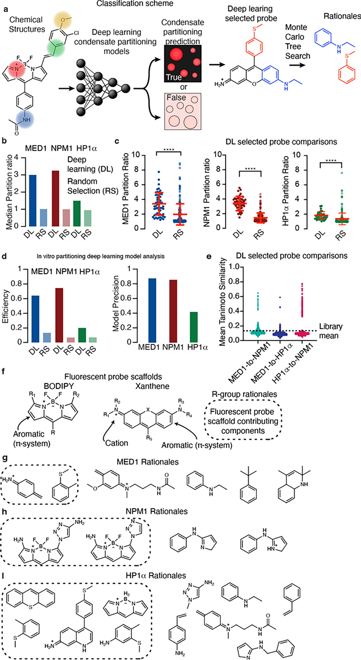
a, Schematic of a message passing neural network for classifying probe partitioning behaviors into in vitro condensates and evaluation of their rationales. b, Bar graph showing the median partition ratio of deep learning (DL) and randomly selected probes (RS). c, Dot plots of partition ratio for fluorescent probes selected by DL or RS in MED1 (DL sample size n = 56, RS sample size n = 224 probes, t=6.6, df = 278), NPM1 (DL sample size n = 50 probes, RS sample size n = 240, t= 17.2, df = 288) and HP1α (DL sample size n = 40 probes, RS sample size n = 240 t= 3.6, df = 278) in vitro condensate assays. Centerline and error bars represent mean ± standard deviation. d, Analysis of in vitro deep learning models, (left) bar graph depicting the efficiency of selecting probes above a condensate’s partition ratio threshold with DL or by RS and (right) a bar graph depicting the precision of deep learning models generated for each condensate (see methods for more information). e, Dot plot showing the Tanimoto similarity of the DL selected fluorescent probes between the condensates considered. f, Chemical structures of fluorescent probe scaffolds. Rationales of fluorescent probe scaffolding (shown in box) and functional groups in g, MED1, h, NPM1, and i, HP1α condensates. (unadjusted p-value, p. **** p < 0.0001,*** 0.0001< p < 0.001, ** 0.001 < p < 0.01, * 0.05 < p < 0.01, evaluated with a two-tailed t-test).
We trained and validated deep learning models on probe structures and binarized probe data for each of the MED1, NPM1, and HP1α protein condensates (Fig. 3a). Models of probe and protein partitioning were subsequently used to predict compounds with selective partitioning behavior from a set of probes withheld from the data for model development. We then used the in vitro condensate imaging assay to measure the partition ratios of predicted high partitioning probes in the withheld set of molecules and, as a control, 240 probes randomly selected from this set (Fig. 3b). A plot of the experimentally determined probe partition ratios showed a shift in the median partition ratio toward higher partitioning for deep learning-selected probes as compared to those probes selected randomly (Fig. 3b–c). These results indicate that deep learning can predict whether small molecules will concentrate in these condensates.
Deep learning was more efficient than random selection by 4-fold (MED1), 10-fold (NPM1), and 3-fold (HP1α) at identifying probes with partition ratios greater than their model training thresholds (Fig. 3d). The greater efficiency of the MED1 and NPM1 models was concomitant with a greater proportion of true positive predictions, or a greater precision (Fig. 3d). To further assess the performance of our deep learning models, we compared the receiver-operator characteristic (ROC) curves of these models to those of Tanimoto similarity calculations and found that deep learning typically outperformed Tanimoto similarity calculations (Extended Data Fig. 6). When comparing probes identified by deep learning for one condensate versus another, at least 90% of the probes had a pairwise Tanimoto similarity less than the library mean, suggesting that the deep learning approach successfully identified chemical features that are discriminating (Fig. 3e). These results demonstrate that the chemical features of small molecules that lead to partitioning into various condensates can be identified with deep learning models and suggest that the rules for chemical features of small molecules that engender attraction to the chemical environment of a specific condensate can be learned and embedded in parameterized representations by neural networks.
The probes predicted to partition into MED1, HP1α, and NPM1 condensates were identified to be primarily xanthene and BODIPY derived fluorophores that possess electron donating R-groups and therefore an electron rich π-system (Fig. 3f). π-Systems may interact strongly with other molecules through their quadrupole moment, forming noncovalent interactions, primarily with cations and other π-systems20–22. MED1 rationales (chemical features) were dominated by aromatic rings functionalized with electron donating, withdrawing, and neutral motifs (Fig. 3g). A preference for the cationic amines and their N-acetyl propylamine derivatives was also found to compose the rationales of MED1 condensate partitioning. Rationales for NPM1 were dominated by aromatic and amine rich moieties, which compose the scaffold of BODIPY dyes predicted to partition into this condensate (Fig. 3h). Analysis of rationales for HP1α revealed aromatic ring structures and building blocks of BODIPY and xanthene dyes (Fig. 3i). These results suggest that cationic and aromatic motifs make an important contribution to the concentrating effects, likely through cation-π and π-π interactions.
Selectivity of condensates for certain small molecules may arise because they favor specific physicochemical properties. We looked for evidence of this by considering probe physicochemical properties that are enriched in high partitioning molecules and found that for the log P, hydrogen bond acceptor count, and number of rotational bonds, these properties were poorly enriched among 90th percentile partitioning probes (Supplementary Fig. 6e–h). We then created classifiers from the physicochemical properties of probes that concentrate at or above the 90th, 75th, and 50th percentile (Supplementary Fig. 8–10). Classifiers were then used to assess performance on a withheld set of fluorescent probes and had at best moderate performance (Supplementary Fig. 8–10f). We then applied a multivariate regression model that takes physicochemical properties and chemical features as input variables (Supplementary Fig. 11). Multivariate linear regression models suggested chemical features and physicochemical properties that were important variables for model training, but do not account for molecular context (Supplementary Fig. 11). In testing these hypotheses, we assume that the performance of a method correlates with the importance of a chemical feature or property towards predicting or describing partitioning behaviors. Deep learning and Tanimoto similarity calculations outperformed other approaches at identifying probes that concentrate in condensates (Extended Data Fig. 6, Supplementary Fig. 8–10f) and could provide important characteristics for high partitioning behavior (Fig. 3g–i). While Tanimoto similarity calculations were able to achieve comparable performance to the HP1α model in vitro, the MPNNs trained here, which combined physicochemical properties and the same chemical fingerprints as Tanimoto, were able to achieve a greater performance at predicting probe partitioning behavior (Extended Data Fig. 6, Supplementary Fig. 8–10f). From these results, we infer that the internal chemical environments of condensates concentrate small molecules that possess a complex ensemble of physicochemical properties and chemical features.
Condensates influence small molecule distributions in cells
We found that simple in vitro condensates formed by key scaffold proteins contain distinct chemical environments that selectively partition small molecules and that deep learning algorithms can predict molecules that selectively partition into these condensates. We wondered whether the chemical environments of these simple condensates might sufficiently reflect the environment in the more complex condensates in living cells such that predictions based on partitioning in vitro might have predictive value in vivo (Fig. 1, 4a, Extended Data Fig. 1, Extended Data Fig. 7, Supplementary Fig. 12). Despite the billions of molecules in cells that could provide competitive interactions, previous studies with simple condensates suggest that such model systems can be predictive of the partitioning behaviors of small and large molecules in the more complex condensates that occur in cells4–11.
Figure 4. Live cell partitioning predicted by deep learning classifiers.

a, Schematic of approach for identifying molecules that concentrate in live cell condensates from in vitro parititoning models. Small molecules were evaluated for in vitro partitioning behavior and then compared to their live cell imaging results. b, Partitioning behavior of small molecules into the nucleolus, (left) dot plot showing nucleolar partitioning behavior of small molecules over background nucleoplasm signal intensity, (right) cumulative distribution function showing the fraction of small molecules that concentrated ( Inucleolus / Ibackground > 2) or did not ( Inucleolus / Ibackground < 2). c, Partitioning behavior of small molecules into chromocenters, (left) dot plot showing chromocenter partitioning of small molecules over background signal intensity, (right) cumulative distribution function showing the fraction of small molecules that concentrated ( Ichromocenter / Ibackground > 2) or did not ( Ichromocenter / Ibackground < 2). d, Receiver-operator curves comparing NPM1 and HP1α models against random chance at classifying drug and natural product partitioning behavior into the nucleolus and chromocenters (see supporting information for more details). e, Bar graphs describing the model performance of NPM1 and HP1α models as compared against a random model diagnostic odds ratio, F1-score, and informed-ness, see Supplementary Table 2 for more information (model accuracy, NPM1: 0.62, HP1α: 0.95) (see supporting information for more details). f, Confocal image of the small molecule mitoxantrone (zoom 4x) in the nucleus of mouse embryonic stem cells. g, Confocal image of the small molecule trypanthrin (zoom 4x) in the nucleus of mouse embryonic stem cells, (a) chromocenter, (b) perinuclear heterochromatin, (c) nucleolus. Scale bar: 10 μm.
Nucleoli and heterochromatic chromocenters are condensates that are easily visualized by confocal microscopy due to their large size, nuclear location, morphology and stability, and thus the relative signal due to concentration of fluorescent small molecules could be reliably measured in these and other large subcellular bodies. NPM1 is a scaffold protein for nucleoli and HP1α is a scaffold protein for heterochromatin condensates, so we investigated the extent to which the deep learning classifier, trained on probe partitioning data from NPM1 and HP1α in vitro condensates (Fig. 2), would correctly predict the nucleolar and chromocenter partitioning behavior.
Of the 10 drugs predicted to concentrate in nucleoli based on training with NPM1 in vitro condensates, 5 were observed to do so, and of the 31 drugs predicted not to concentrate in nucleoli, 11 appeared to concentrate in these bodies (Fig. 4b, Supplementary Table 2). This reveals that the model’s predictions for the nucleolar condensate in living cells are less successful than those for the simple in vitro condensate, yet the model was 63% accurate and 2.1-fold better at correctly predicting high-partitioning small molecules than an averaged random selection process, as determined by their diagnostic odds ratio (see supporting information for details). Of the 5 drugs predicted to concentrate in chromocenters, 4 were observed to do so (Fig. 4c, Supplementary Table 2); among 36 other drugs tested that were not predicted to concentrate in chromocenters, only daunorubicin was found concentrated in these bodies (Supplementary Fig. 12). Calculation of ROC curves demonstrated that NPM1 and HP1α deep learning models had modest performance at predicting partitioning behavior in live cells, but they outperformed a standard Tanimoto similarity approach (Fig. 4d, Extended Data Fig. 8). These results show that the HP1α deep learning classifier was 95% accurate and 140-fold better at correctly predicting high partitioning small molecules than an averaged random selection process, as determined by their diagnostic odds ratio (Fig. 4e). Thus, the HP1α deep learning classifier outperformed the NPM1 model, and both classifiers outperformed a random selection process (Fig. 4e). The compounds that exhibited the highest levels of partitioning in this assay were mitoxantrone (in nucleoli) and tryptanthrin (in chromocenters). Mitoxantrone, a potent chemotherapeutic23, appeared to concentrate up to 6-fold above the surrounding nucleoplasm (Fig. 4f, Extended Data Fig. 9a). Tryptanthrin, an alkaloid with broad biological activities24, appeared to concentrate in chromocenters (Extended Data Fig. 9b) up to 25-fold over the surrounding nucleoplasm and over 42-fold over the nucleolus (Fig. 4g, Extended Data Fig. 9c). Thus, the deep learning algorithm, trained on simple in vitro condensates, was able to predict that some drugs will selectively concentrate in the more complex environment of the relevant condensates in cells, albeit with limited accuracy. In summary, our results suggest that the interaction between small molecules and the chemical environments of simple in vitro condensates can be somewhat predictive of small molecule interactions with more complex condensates in living cells.
Discussion
We find that small molecule therapeutics tend to concentrate in distinct intracellular compartments and that biomolecular condensates contain distinct chemical solvation environments that can selectively concentrate small molecules. We also find that the chemical features of small molecules that engender attraction to the chemical environment of a specific condensate can be predicted by using deep learning with small molecule probes. These results have important implications for our understanding of molecular distributions within cells and for improving the pharmacological activity of therapeutics.
Much of our understanding of biological regulatory mechanisms has been established by identifying the collection of protein and other biomolecules that bind to one another with high affinity (e.g., Kd between 100 pM – 1 μM) relative to their interactions with other biomolecules, thus producing complexes of specific molecules with a certain stoichiometry and stability. By contrast, dynamic, multivalent low affinity interactions generated by the ensemble of diverse biomolecules in condensates can produce distinct internal chemistries. The different chemical environments of biomolecular condensates may thus confer additional specificity on biological regulatory processes beyond those obtained through canonical high-affinity interactions.
The evidence that condensates harbor distinct chemical environments implies that the selective incorporation of specific biomolecules into particular condensates is likely to be governed both by the solvation environment produced by the ensemble of components in the condensate and by high-affinity interactions with other biomolecules. These results suggest that the molecules are subjected to both of types of chemical forces to ultimately reside in appropriate compartments where they are concentrated together with their partners to carry out shared activities. Similarly, these results imply that both chemical forces contribute to selective concentration of drugs in specific intracellular compartments.
The chemical solvation properties of simple in vitro protein condensates, inferred by deep learning, could be used to predict with some accuracy the tendency of small molecule drugs to concentrate in the more complex condensate where that protein serves as a scaffold in living cells. It is possible that the scaffold proteins selected for study tend to dominate the chemical environment in the more complex cellular condensate and/or tend to interact with other proteins or nucleic acids that favor similar chemical environments.
We considered several mechanistic models that might account for selective small molecule concentration in condensates. Condensates may concentrate small molecules through the creation of a ‘mean field’ chemical solvation environment, wherein a general solvent quality leads to the partitioning of molecules that share a specific chemical property (Fig. 5a). A mean field solvation effect might be anticipated if, for example, compounds with a particular degree of hydrophobicity are selectively concentrated in condensates. The concentration of compounds within condensates might also reflect the creation of local chemical environments between associating biopolymers that effectively create “chemical pockets” that selectively concentrate small molecules (Fig. 5b). Local chemical environments that act as pockets to solvate small molecules can be created by the dynamic association of portions of polymers and might be anticipated to concentrate a more diverse set of chemistries than those of a mean field. A third model arises by considering that scaffolding proteins may in part adopt folds or structures upon partitioning into condensates that create high affinity binding sites (Fig. 5c). Finally, condensate scaffolding proteins may be liganded by molecules inside and outside of the condensate, and concentrate them within the condensate because the protein itself is highly concentrated within (Fig. 5d). A high affinity binding site, created within the condensate and not present outside of the condensate or orders of magnitude more concentrated inside the condensate, would be anticipated to concentrate a particular ligand structure (e.g, a pharmacophore), or a set of ligand structures. These mechanistic models are not mutually exclusive and different condensates may concentrate molecules through a model that is optimal for its specific biochemical processes.
Figure 5. Small molecule-protein interactions in condensates.

Internal chemical environments in condensates selectively concentrate small molecules. a, Internal chemistry of condensates could concentrate molecules simply because their internal environment differs by a classic bulk phase property (e.g., dielectric constant). b, Association of polymers could lead to the creation of local chemical environments or “chemical pockets” that concentrate small molecules. c, Concentration of a protein into a condensate could lead to changes in the ensemble of states occupied by a biopolymer, creating a high affinity small molecule binding site. d, Small molecules and proteins could bind through the same structures inside and outside a condensate, such that increase in protein concentration inside of the condensate effectively concentrates the small molecule.
One model for protein interactions in condensates invokes the concept of “sticker” regions, patches of amino acids, often in intrinsically disordered regions, that together define a specific chemical character such as positive charge, negative charge, hydrophobicity, etc 25–27. Regions with complementary character, such as a patch of positively charged amino acids and a patch of negatively charged amino acids, might then contribute to interactions between and among the biopolymers13, 25–27. Such patches might also be expected to contribute to interactions with small molecules, and would be consistent with the “chemical pocket” model described above, where many different pockets might be formed within the same condensate. In this model, small molecule partitioning results from interactions between small molecules and a diverse ensemble of many different interactions provided by the protein. This ensemble could encompass a highly diverse range of possible conformations of protein along with the range of potential orientations of molecule and protein.
The mutual concentration of small molecule therapeutics and their target proteins in a specific condensate would be expected to create optimal therapeutic efficacy. However, we observed multiple instances where a therapeutic did not concentrate in the location of its target protein. Drug uptake into compartments that do not contain the target may lead to off-target interactions and, in some cases, toxicity. We propose that through improved understanding of condensate chemical grammar, the chemical features of a drug might be optimized to enhance its concentration in target-containing condensates while reducing its concentration in off-target compartments, resulting in small molecule therapeutics with improved pharmacodynamic profiles.
Materials and methods:
Tumor cell tissue culture
Human colorectal cancer cells (HCT-116 American Tissue Culture Catalog CCl-247™), prostate cancer cells (PC3 American Tissue Culture Catalog CCl-1435™), and breast cancer cells (MCF7 ATCC HTB-22 ™) were cultured in sterile 10 or 15 cm plates with 15 or 35 mL of DMEM (Gibco, 11965084) media supplemented with 10 % Fetal bovine serum (FBS) (Sigma F2442) and 100 units/mL penicillin (Life Technologies, 15140122), and 100 μg/mL streptomycin (Life Technologies, 15140122). Cells were cultured at 37 °C and 5 % v/v CO2 in a humidified cell culture incubator and passaged at 75 % confluency. Cells were counted to determine seeding density using a Countess™ II automated cell counter, employing trypan blue and disposable countess chamber slides according to manufacturer recommendations. Cells were tested regularly for mycoplasma using the MycoAlert Mycoplasma Detection Kit (Lonza LT07–218) and found to yield negative results. HCT-116 cells expressing MED1-, NPM1-, and HP1α -GFP from the endogenous gene locus were previously reported3.
Mouse embryonic stem cell tissue culture
V6.5 mouse embryonic stem cells (mESCs) were a kind gift from R. Jaenisch, and were authenticated by STR analysis compared to commercially acquired cells with the same name. Stem cells were cultured in 2i/LIF medium on tissue culture-treated plates coated with 0.2 % gelatin (Sigma G1890) in a humidified incubator at 37 °C and 5 % CO2. Cells were passaged every 1–2 days by dissociation using TrypLE Express (Gibco 12604) and the dissociation reaction was quenched using serum/LIF medium. Cells were tested regularly for mycoplasma using the MycoAlert Mycoplasma Detection Kit (Lonza LT07–218) and found to yield negative results.
2i/LIF medium is defined as 3 μM CHIR99021 (Stemgent 04–0004), 1 μM PD0325901(Stemgent 04–0006), and 1000 U−1mL leukemia inhibitor factor (LIF, ESGRO ESG1107) in N2B27 medium.
The composition of N2B27 medium is as follows: DMEM/F12 (Gibco 11320) supplemented with 0.5-fold N2 supplement (Gibco 17502), 0.5-fold B27 supplement (Gibco 17504), 2 mM L-glutamine (gibco 25030), 1-fold MEM non-essential amino acids (Gibco 11140), 100 U−1mL penicillin-streptomycin (Gibco 15140), and 0.1 mM 2-mercaptoethanol (Sigma m7522).
Serum/LIF medium was prepared from KnockOut DMEM (Gibco 10829) supplemented with 15 % fetal bovine serum (Sigma F4135), 2 mM L-glutamine (Gibco 25030), 1-fold MEM non-essential amino acids, 100 U−1mL penicillin-streptomycin, 100 μM 2-mercaptoethanol (Sigma M7522) and 1000 U−1mL LIF (ESGRO ESG1107).
Instrumentation
Droplet images were recorded with an Andor Revolution spinning disk confocal microscope using a 1.4 NA 100x Plan Apo objective and a 150x zoom function in screening mode. Data was collected using MetaMorph acquisition software, version 7.8. The Andor revolution was outfit with an Andor iXion+EMCCD camera and excitation lasers at 405 nm 50 mW, 488 nm 50 mW, 561 nm 50 mW, 640 nm 100 mW. Emission intensity was collected with bandpass EM-CCD band pass filters 405 nm (447/60nm), 488 (525/40nm), 561 (617/73nm), 640 (685/41nm). Excitation intensity was maintained constant throughout all screening experiments.
Live cell confocal micrographs were recorded with a Zeiss LSM 980 Airyscan 2 Laser Scanning confocal operating in super resolution mode with a 1.4 NA 63X Plan Apo objective and running Zeiss Zen Blue V. 3.5. Cells were maintained at 37 °C and 5 % v/v CO2 in a humidified chamber throughout the experiment with accompanying atmospheric controls. Images were recorded using 405 nm 25 mW, 488 nm 25 mW, 561 25 mW, or 639 nm 25 mW diode laser. Excitation intensity was adjusted according to analyte brightness.
Live cell Two-photon micrographs were recorded with a Zeiss LSM 710 Laser Scanning confocal operating in 2-photon mode with a 1.4 NA 63X Plan Apo Objective. Cells were maintained at 37 °C and 5 % v/v CO2 in a humidified chamber throughout the experiment with accompanying atmospheric controls. Images were recorded using Coherent Chameleon Ultra II femtosecond pulsed-IR laser, tuned to 750 nm. Excitation intensity was adjusted according to analyte brightness. Images were averaged twice.
Live cell imaging
HCT-116 cells or endogenously tagged NPM1-GFP HCT-116 cells were seeded at 200,000 cells/mL on an imaging plate. Imaging plates used were sterile Cellvis 96-well glass (Cellvis, P96–1.5H-N) bottom plates with #1.5 high performance cover glass (0.17 ± 0.005 mm), or sterile Cellvis 384-well (Cellvis, P384–1.5H-N) glass bottom plates with #1.5 high performance cover glass (0.17 ± 0.005 mm).
Cells were plated 24 hours prior to the experiment. Prior to imaging, cells were washed once with fresh DMEM (Gibco, 11965084) supplemented with FBS/PS (Life Technologies, 15140122), 4.5 g/L glucose, 110 mg/mL sodium pyruvate, and 584.4 mg/mL L-glutamine. Then a premixed solution of analyte at a given concentration was prepared at a concentration of 5 to 100 μM in DMEM supplemented with FBS/PS and then incubated with cells. The analyte solution was allowed to incubate with the cells for 60 minutes at 37 °C and 5 % v/v CO2, prior to a final wash and application of fresh DMEM supplemented with FBS/PS followed by imaging. Cells were maintained at 37 °C with 5 % v/v CO2 in a humidified chamber over the course of the imaging experiment.
Mouse embryonic stem cells were imaged on sterile Cellvis 96-well glass (Cellvis, P96–1.5H-N) bottom plates with #1.5 high performance cover glass (0.17 ± 0.005 mm), or sterile Cell vis 384-well (Cellvis, P384–1.5H-N) glass bottom plates with #1.5 high performance cover glass (0.17 ± 0.005 mm). These plates were coated with poly-L-ornithine (Sigma P4957) for 30 minutes at 37 °C followed by a coating with 20 μg/mL laminin (Corning 354232) for 2 hours at 37 °C. Cells were maintained at 37 °C with 5 % v/v CO2 in a humidified chamber over the course of the imaging experiment.
Small molecule fluorescent probe library
The small molecule fluorescent probe library consisted of a pool of 6000 fluorescent dyes. The library consisted of xanthene, boron dipyrromethene (BODIPY), and cyanine dyes. These dyes were prepared through combinatorial chemistry employing a range of R-groups sampling a range of chemistry including: alkyl, alkenes, aromatic rings, sulfonamides, nitriles, N,S, and O mono- and di-substituted heteraromatic rings (5- and 6-membered), alkyl, aryl, and heteroaryl hydroxyl groups, alkyl, aryl and heteroaryl halogens, alkyl and aryl methoxy groups, alkyl and aryl ethoxy groups, alkyl subtitued aromatic and heteroaromatic rings (5- and 6-membered), alkyl, aryl, and heteroaryl carbonyl compounds, 1,2,3-triazoles, primary amines, secondary amines, tertiary amines in linear and saturated carbocycles, esters, trichloroacetyl esters, trifluoroacetyl esters. Compounds were derivatized to incorporate a primary alkyl or aryl amine, alkyl or aryl acetamide, or an alkyl or aryl chloroacetyl moiety on the 5,3, or 8 position of the BODIPY dye, 3,6, or 9 position of xanthene dyes. Xanthene dye scaffolds consisted of rhodamine, rhodol, fluorescein, thioxanthene, and N-substituted xanthenes. BODIPY probes were modified at the 5,3, and 8 positions. Xanthene dyes were modified at 3,6, and 9 positions of the ring. Cyanine dyes were modified at the heteroaromatic nitrogen atom and conjugated to a linker substituted with additional chemical motifs. Selection of probes for experiments was made by the fluorophore and microscope optical constraints. Fluorescent probes were maintained at a concentration of 10 mM in DMSO and stored at −80 °C.
Small molecules
All small molecules were received from the vendor and used without further purification. Actinomycin D (Sigma Aldrich A1410), amiloride (Fisher Scientific 0890100), amlexanox (Fisher Scientific A24011G), amsacrine (VWR 76325–752), apigenin (APExBio L1021), baicalein (APExBio L1021), bedaquiline (APExBio L1021), berbamine (APExBio L1021), berberine (APExBio L1021), bosutinib (Sigma Aldrich PDZ0192), broxyquinoline (APExBio L1021), camptothecin (APExBio L1021), cinchonidine (APExBio L1021), clofazimine (Sigma Aldrich C8895), daunorubicin (Thermo Fisher Scientific 251800), diacerein (APExBio L1021), dibucaine (APExBio L1021), epalrestat (APExBio L1021), ethacridine (APExBio L1021), etretinate (APExBio L1021), gentian violet (APExBio L1021), isorhamnetin (APExBio L1021), kaempferol (APExBio L1021), linsitinib (APExBio L1021), mitoxantrone (Sigma Aldrich M6545), piperine (APExBio L1021), proflavine (Sigma Aldrich P2508), psoralen (APExBio L1021), quinine (APExBio L1021), rutin (APExBio L1021), scutellarin (APExBio L1021), suramin (APExBio L1021), Sunitinib malate ( Cayman Chemical 13159), tanshinone I (APExBio L1021), tanshinone II (APExBio L1021), triamterene (APExBio L1021), topotecan (Fisher Scientific NC0707744), tryptanthrin (Sigma Aldrich, SML0310) wedelolactone (APExBio L1021), and XL-765 (APExBio L1021). Small molecules were stored at −80 °C.
Recombinant protein expression and purification
Scaffolding and blue fluorescent protein fusions were constructed as previously described3. For protein expression plasmids were transformed into LOBSTR cells (a kind gift of Cheeseman Lab) and grown as follows. A fresh bacterial colony was inoculated into LB media containing kanamycin and chloramphenicol and grown overnight at 37 °C. Cells were diluted 1:30 in 500 mL room temperature LB with freshly added kanamycin and chloramphenicol and grown 2.5 hours at 16 °C. IPTG was added to 1 mM and growth continued for 20 hours. Cells were collected and stored frozen at −80 °C.
Pellets from 500 mL cells were resuspended in 15 mL of Buffer A (50 mM Tris pH7.4, 500 mM NaCl), complete protease inhibitors (Roche, 11873580001) and sonicated (ten cycles of 15 seconds on, 60 sec off). The lysate was cleared by centrifugation at 12,000g for 30 minutes at 4 °C and added to 1 mL of Ni-NTA agarose (Invitrogen, R901–15) pre-equilibrated with 10X volumes of buffer A. Tubes containing this agarose lysate slurry were rotated at 4 °C for 1.5 hours. The slurry was centrifuged at 1,500g for 10 minutes. The resin was washed with 2 X 5 mL of Buffer A followed by 2 X 5 mL Buffer A containing 50 mM imidazole. The protein was eluted by rotating 3 X with 2 mL of Buffer A containing 250 mM imidazole incubating for 10 or more minutes each cycle at 4 °C. Each eluate was run on a 12% Bis-Tris acrylamide gel. Fractions containing protein of the correct size were dialyzed against two changes of buffer containing 50 mM Tris 7.4, 500mM NaCl, 10% glycerol and 1 mM DTT at 4 °C. Any precipitate after dialysis was removed by centrifugation at 1,500g for 10 minutes.
Homotypic in vitro droplet assay
Recombinant MED1-BFP, HP1α -BFP, and NPM1-BFP fusion proteins were purified and concentrated to 50 μM as described above. Protein was added to a droplet formation buffer consisting of 50 mM Tris HCL, 1 mM DTT, 125 mM NaCl, 10% 8 kDa polyethylene glycol crowding agent at pH 7.5. A Tecan Evo 150 or a Beckman Echo 655 liquid handler was used to dispense 50 nL of fluorescent probe from a master plate containing fluorescent probes at 10 mM in DMSO, to a solution of 1 μL 50 μM protein and 9 μL droplet formation buffer as described above to provide a final probe and protein concentration of 50 and 5 μM respectively. The plate was sealed with parafilm, protected from light and incubated at 37 °C overnight to equilibrate the sample. After equilibration, droplet images were recorded at room temperature using the plate screening mode with the Andor microscope as described above. In total, 11 images were recorded for each fluorescent probe at different locations within the image with 500 ms exposures and a normalized laser power.
Droplet image analysis
Droplet image analysis was performed using an in-house developed Python script. Briefly, a binary mask was generated from the 405 nm or protein channel signal that was of at least 25 pixels in size and with intensity values above the background of each image (droplets were detected from the 405 nm excitation channel). The intensity of the fluorescent probe was measured within and outside of the regions demarcated by this mask in the fluorescent probe channels (488, 561, 640 nm) and averaged. The concentration of a fluorescent probe was assumed to be proportional to the intensity of the fluorescent probe inside and outside of the binary mask, and the partition ratio, K, was computed as Intensity ≈ C, for C = Cin or Cout as defined by the binary mask. The partition ratio used here is the quotient of these values Cin/Cout = K. The total number of probes used in MED1, NPM1 and , HP1α droplets were 1143, 1055, and 963 molecules, respectively. Measurements of protein partition ratio were assessed by evaluation of the fluorescent signal intensity inside and outside of the mask using the 405 nm channel. Measurements of condensate circularity were performed using scikit-image measure package on the computed masks from the 405 nm channel.
Chemoinformatics
Fluorescent probe chemical structures were generated as SMILES strings and sanitized. Pairwise Tanimoto similarity calculations were performed using Morgan Fingerprints with a radius of 2 in a 2048-bit depth as implemented in the program RDKit (v2021.03.2)28. Calculations of log P, hydrogen bond acceptor count, number of rotatable bonds, topological polar surface area, molecular weight were computed with RDKit (v2021.03.2)28.
Calculation of receiver-operator curves
Receiver operator curves were computed using binary classification criteria for each probe and partition ratio as the ground truth using the scikit-learn metrics module29.
Tanimoto similarity classifiers
Tanimoto similarity classifiers were constructed from probes that had measured partition ratios in the 90th percentile of probe partitioning data for each condensate. These sets of probes were used to compute Tanimoto similarity metrics with other probes, drugs, and natural products. Fluorescent probes that had computed Tanimoto similarities above various thresholds: Tanimoto similarity = 0.50, 0.75, 0.80, 0.85 were noted as ‘true’ and those below these values were computed as ‘false.’ Natural products and drugs were classified using a Tanimoto similarity threshold of 0.5, above this threshold natural products and drugs are labeled as ‘true’ and below ‘false.’ These data were then plotted in a receiver operator curve (see Calculation of receiver-operator curves for more details). Tanimoto similarity calculations were performed as described in the chemoinformatics section of the methods.
Structure-activity relationships
Probes were identified from our data sets for the generation of structure-activity relationships by identifying groups of probes with a shared dye scaffold (i.e., cyanine, xathene, or BODIPY) and evaluating by inspection the effect of different chemical features (e.g, aromatic rings, heteroaromatic rings, alkanes) on the partition coefficient of each molecule.
Physicochemical property classifiers
Probe physiochemical property classifiers were constructed at or above three different threshold ranges: the 50th percentile, 75th percentile, and 90th percentile of the data. Probes that had partition ratios in each threshold range were split into a group that composed 80 % and 20 % of the probes. The 80 % population was used to define the physicochemical property range for Log P, topological polar surface area (TPSA), number of hydrogen bond acceptors (HAcc), the number of rotational bonds (RotB), and the molecular weight (MW). Physicochemical property ranges were defined by taking the average and computing a standard deviation and the range was defined: physicochemical property range = (average of property) ± (standard deviation of property). These ranges were computed separately for each threshold. Whole numbered physicochemical properties such as those for the number of rotational bonds and hydrogen bond acceptors were rounded to the nearest whole number. The remaining 20 % of probes from the threshold probe set and all other data were combined and classified using the physicochemical range classifier. Each classifier was applied independently and individual physiochemical properties were classified as ‘true’ when they were contained within a physicochemical property range and ‘false’ when they were outside of a physicochemical property range. These data were then plotted in receiver operator curves (see Calculation of receiver-operator curves for more details). The physicochemical property ranges defined are as follows. MED1 physicochemical property ranges, 90th percentile: Log P = 6.5 ± 1, TPSA= 60 ± 20, HAcc = 4 ± 1, RotB = 7 ± 4, MW= 537 ± 102. MED1 physicochemical property ranges, 75th percentile: Log P = 6.0 ± 1.5, TPSA= 60 ± 20, HAcc = 4 ± 2, RotB = 7 ± 3, MW= 520 ± 100. MED1 physicochemical property ranges, 50th percentile: Log P = 5.8 ± 1.5, TPSA= 60 ± 20, HAcc = 4 ± 2, RotB = 7 ± 3, MW= 520 ± 100. NPM1 physicochemical property ranges, 90th percentile: Log P = 5.9 ± 1.7, TPSA= 72 ± 24, HAcc = 5 ± 2, RotB = 8 ± 4, MW= 372 ± 60. NPM1 physicochemical property ranges, 75th percentile: Log P = 5.9 ± 1.7, TPSA= 68 ± 22, HAcc = 5 ± 2, RotB = 7 ± 4, MW= 415 ± 134. NPM1 physicochemical property ranges, 50th percentile: Log P = 5.7 ± 1.5, TPSA= 63 ± 33, HAcc = 4 ± 2, RotB = 7 ± 4, MW= 505 ± 215. , HP1α physicochemical property ranges, 50th percentile: Log P = 6.52 ± 1.6, TPSA= 70 ± 22, HAcc = 5 ± 2, RotB = 8 ± 4, MW= 569 ± 110. , HP1α physicochemical property ranges, 50th percentile: Log P = 6.4 ± 1.5, TPSA= 66 ± 22, HAcc = 5 ± 2, RotB = 7 ± 4, MW= 559 ± 109. , HP1α physicochemical property ranges, 50th percentile: Log P = 6.2 ± 1.4, TPSA= 65 ± 23, HAcc = 4 ± 2, RotB = 7 ± 4, MW= 546 ± 106.
Partial least squares regression model analysis
Partial least squares regression (PLSR), also known as projection to latent structures regression, was performed using the “pls” package30 (v. 2.8.0) in R (v. 4.1.0) 31. Separate models were created for MED1, HP1α, and NPM1 partitioning data. For each model, a feature matrix X was constructed using bit-encoded Morgan fingerprints (discrete-valued) as well as gross physicochemical properties (continuous- or discrete-valued). This matrix was filtered to remove molecular fingerprint features consisting of fewer than 9 nonzero entries. A vector Y was composed of the experimentally determined log10(K) for each molecule.
PLSR was employed to model the multivariate relationship between X and Y using the ‘plsr’ function in “pls” with X scaling. The dataset was first randomly segmented into a training set (80%) and test set (20%). The training set was modeled with 10-fold cross validation to calculate the cross-validation mean square error (MSE) of prediction. Cross-validation was performed using different numbers of latent variables to determine the optimal number of components where MSE was minimized. The optimized training set model was then applied to the test set to calculate a test set MSE. Subsequently, the full dataset was modeled using the optimal number of latent variables to generate plots, calculate variable importance in projection (VIP), and calculate regression coefficients. VIP values were calculated using the “plsVarSel” R package (v. 0.9.7) 32, while regression coefficients were calculated using the ‘coeff’ function in “pls”.
The importance of features (chemical properties and fingerprints in the model) was assessed using a strategy incorporating regression coefficients and VIPs. For physicochemical properties, features with VIP>1 were retained, then these features were ranked according to the regression coefficient. The four properties with the highest coefficients (most positive) were determined to be important predictors of high partitioning in a given condensate. Likewise, the four properties with the lowest coefficients (most negative) were determined to be negative predictors of partitioning. A similar strategy was used to select Morgan fingerprints, excluding groups that are exclusively part of the scaffold.
PLSR models for MED1, HP1α, and NPM1 were separately validated by comparison to randomly permuted null models. Each model was constructed 100 times using random train-test splits. Training set MSEs were calculated using 10-fold cross validation and test set MSEs were calculated from the prediction error in each instance of the model. Using the same train-test splits, null models were generated by randomly permuting the entries of the outcome variable Y. Corresponding training and test set MSEs were calculated for the permuted models as described above. The statistical significance of the true model was analyzed by comparing the MSE distributions (n=100) between the true and null models via the Mann-Whitney U-test. Separate statistical tests were conducted on MSE distributions originating from training and test sets.
Machine learning
Datasets quantifying the partitioning of small molecules in MED1, NPM1 and HP1α droplets were collected, consisting of 1143, 1055, and 963 molecules, respectively. To predict the partitioning ratio of molecules, we trained a random forest classifier and a directed message-passing neural network (MPNN) separately and aggregated their predictions. Given a molecule’s SMILES string, the models aimed to predict if the molecule’s partition ratio was above a preset threshold. We selected a threshold for each condensate: 2.7 for MED1, 2.7 for NPM1, and 2.0 for HP1α to select compounds which partition into a condensate, or not.
The random forest classifiers were trained using the scikit-learn package29 (v0.24.2) in Python (v3.8.10), setting “n_estimators” to 200, “min_samples_leaf” to 2, and “n_jobs” to 4. Each molecule was transformed into a 1024-dimensional vector using the Chem.RDKFingerprint method from the open-source package RDKit (v2021.03.2).28 Each classifier was trained on 90% of the data. To train the MPNN models on the classification tasks, we used Chemprop (v1.3.1). 33 The models took as input both the SMILES string representation of each molecule as well as a 200-dimensional vector generated using Chemprop and setting “features_generator” to rdkit_2d_normalized. Molecules were assigned to either the training set (80 %), validation set (10 %), or test set (10 %) using a scaffold split. All MPNNs were trained with a batch size of 50 for 50 epochs with an ensemble of 10 models per task.
Predictions for a held-out dataset of 1,498 fluorescent molecules were determined by majority voting. A molecule’s partitioning ratio was predicted to be above a given threshold if both the random forest and MPNN models predicted a score greater than 0.5 and was predicted below the given threshold otherwise.
Efficiency calculation
We estimated the efficiency of our models to identify probes with desired partitioning behavior by adapting the expression used to evaluate the efficiency, , of a combustion engine as shown in equation (1).
| (1) |
Where variable is a count of the number of probes with a partition ratio above a threshold (here, K > 2.0), for a machine learning model. The variable is the total number of probes. These calculations were performed with a combined sample size of 300 fluorescent probes, including those that were selected by our deep learning models for each condensate (60 probes, DL) and those identified by selecting probes at random (240 probes, RS).
Chemical rationales of partitioning
Our approach follows a previously published methodology. 34 Probes predicted to concentrate into a condensate by each condensate’s MPNN are used to ask what subgraphs (chemical features or rationales) of each molecular graph contribute to the partitioning behavior of a molecule. Subgraphs were extracted using the interpretability functionality of the chemprop package. We applied a significance threshold to classify contributions to the MPNN score for subgraphs, MED1 (0.50), NPM1 (0.50), and HP1α (0.25). All other parameters were set to their default values.
Drug nucleolar enrichment
Images were then recorded as described above using a confocal or two-photon microscope and analyzed using Fiji (V.2.3) 35. A drug was classified as enriched if a distinct nucleolar pattern could be observed in a cell and considered as unenriched if a nucleolar pattern could not be observed. We measured the intensity of signal from endogenously fluorescent drugs in regions discernable as the nucleolus across 3 different images and between 5–15 cells to compute in the intensity of light in the nucleolus, In, and compared it to the intensity of the light in the nucleoplasm to describe a molecule as enriched if the mean In / Inp > 2. Enriched or unenriched populations of each molecule were then used in the statistical analyses of the model’s performance (See Supplementary Table 2 and statistical analysis).
Drug chromocenter enrichment
Cells were treated with Hoechst 33342 at 0.1 μg/mL and 50 μM of an endogenously fluorescent small molecule in 2i/LIF media for 10 minutes at 37 °C and 5 % CO2 in a L-ornithine and laminin treated glass bottom plate or dish. Cells were then taken out of the incubator, washed twice with fresh 2i/LIF media and fresh 2i/LIF media was placed on the cells. Images were then recorded as described above using a confocal or two-photon microscope and analyzed using Fiji. At least fifty chromocenters were analyzed across 5–10 images by selecting large punctate structures demarcated by Hoechst 33342 stain and the intensity of signal in these objects (Ichromocenter) was measured in the 405 nm and 488, 561, or 639 nm channels to assess the presence of Hoechst or the drug respectively. The background intensity (Ibackground) was determined by selecting 50 regions in different cells where the nucleus not marked by Hoechst stain (or determined to be chromocenters, in the case of tryptanthrin), and the intensity of signal in these regions was measured using the 405 nm and 488, 561, or 639 nm channels to assess the presence of Hoechst or the drug respectively. Chromocenter partitioning was evaluated by taking the ratio of Ichromocenter / Ibackground, and a chromocenter was considered enriched in a drug if Ichromocenter / Ibackground > 2 (data shown in Fig. 4c). The signal intensity ratio from each molecule chromocenter was then used in the assessment of model performance (See Supplementary Table 2 and statistical analysis).
Statistics and reproducibility
All statistical tests were performed using GraphPad Prism (v. 9.2.0). Comparisons between partition ratio percentile distributions were analyzed using a two-tailed Wilcoxon matched-pairs signed rank test. Differences in mean Tanimoto similarity distributions were made using an unpaired two-tailed t-test. Adjustments were not made for multiple comparisons. To assess classifier performance on nucleolar and chromocenter enrichment (Supplementary Table 2), the metrics of accuracy (), balanced accuracy (), F1-score (), informed-ness (), and diagnostic odds ratio () were computed using equations (2–8).
| (2) |
| (3) |
| (4) |
| (5) |
| (6) |
| (7) |
| (8) |
The F1 score is a measure of classifier’s accuracy, it is useful when a class imbalance is present (when the number of true positives/negative and false positives/negatives is skewed). Informed-ness (or Youden’s J statistic) provides a statistic that captures the performance of a diagnostic test, here, the ability of the classifier to successfully predict a probe’s partitioning behavior.
With TP = True positive, TN = True negative, FP = False positive, FN = False negative. The 95% confidence interval for was computed assuming that the ln() followed a normal distribution.
A true positive (TP) is defined, nucleolar / chromocenter enrichment = yes and prediction of NPM1/ HP1α = true, a false positive (FP) is defined, nucleolar / chromocenter enrichment = no and prediction of NPM1/ HP1α = true. And a true negative (TN) is defined, nucleolar / chromocenter enrichment = no and prediction of NPM1/ HP1α = false. A false negative (FN) is defined, nucleolar / chromocenter enrichment = yes and prediction of NPM1/ HP1α = false.
Analysis of the NPM1 model and experimental results (Supplementary Table 2) provided the following inputs, TP = 5, FP = 5, FN = 10, and TN = 21 and thus we found a TPR = 0.33, TNR = 0.81, an accuracy (ACC) = 0.63, balanced accuracy (BA) = 0.57, F1 = 0.40, an informed-ness (I) = 0.14, DOR = 2.1 (95 % CI, 0.49 – 8.95). The NPM1 model was 10% more accurate than a random model as computed below, and had a 2-fold greater DOR.
Analysis of the HP1α model and experimental results (Supplementary Table 2) provided the following inputs, TP = 4, FP = 1, FN = 1, TN = 35, and thus we found a TPR = 0.80, TNR = 0.97, an accuracy (ACC) = 0.95, balanced accuracy (BA) = 0.88, F1 = 0.80, an informed-ness (I) = 0.77, DOR = 140 (95 % CI, 7 – 2,697). The HP1α model was 45 % more accurate than a random model as computed below, and had a 140-fold greater DOR.
We compared the DOR of the NPM1 and HP1α models to a ‘random model’ defined such that pool of compounds was a total of 40 split evenly across each different input, i.e., TP = TN = FP = FN = 10, which provides a DOR = 1 and an accuracy of 0.50.
For the biological experiments performed here, at least 3 biological replicates were collected. In each biological replicate of microscopy assays, 3–5 images were recorded, typically with at least 4–5 cells in each micrograph. Representative images were selected by inspection of each phenotype in each cell line.
Extended Data
Extended Data Figure 1. Live cell confocal and two-photon imaging of endogenously fluorescent drugs.

HCT-116 cells were incubated with a drug or natural product at 50 μM for 1 hour and then imaged with a confocal or two-photon microscope. Image for sunitinib is also shown in Figure 1. Scale: 10 μm.
Extended Data Figure 2. Subcellular distribution of small molecules in a breast cancer cell line.

Live MCF7 cells were incubated with a drug or natural product at 50 μM for 1 hour prior to confocal imaging. Scale: 10 μm R = CH2CH2OCH2CH2NH2, R2 = CH2CH2N(CH2CH3)2.
Extended Data Figure 3. Subcellular distribution of small molecules in a prostate cancer cell line.

Live PC3 cells were incubated with a drug or natural product at 50 μM for 1 hour prior to confocal imaging. Scale: 10 μm. R = CH2CH2OCH2CH2NH2, R2 = CH2CH2N(CH2CH3)2.
Extended Data Figure 4. Additional analysis of condensate selectivity in fluorescent probe partitioning.

(a-c) Dot plots comparing the partition ratios of probes above the 90th percentile in, a, MED1, b, NPM1, and c, HP1α against their partition ratios in other condensates. p-values computed with a two-sided unpaired t-test, n=50 and df=98 for all groups, with t-statistics and effect sizes (η2) as follows: MED1-NPM1 (t=22.87, η2=0.84), MED1- HP1α (t=19.88, η2=0.80), NPM1-MED1 (t=3.43, η2=0.11), NPM1- HP1α (t=8.24, η2=0.41), HP1α -MED1 (t=3.15, η2=0.09), HP1α -NPM1 (t=4.09, η2=0.15). (d-f) Dot plots comparing the partition ratios of probes below the 10th percentile in d, MED1, e, NPM1, and f, HP1α against their partition ratios in other condensates. p-values computed with a two-sided unpaired t-test, n=50 and df=98 for all groups, with test statistics as follows: MED1-NPM1 (t=3.79, η2=0.13), MED1- HP1α (t=4.65, η2=0.18), NPM1-MED1 (t=3.12, η2=0.09), NPM1- HP1α (t=2.60, η2=0.07), HP1α -MED1 (t=3.76, η2=0.13), HP1α -NPM1 (t=4.20, η2=0.15). (g-i) Dot plots comparing the percentile ranks of probes below the 10th percentile in g, MED1, h, NPM1, and i, HP1α against their percentiles in other condensates. p-values computed with a two-sided Wilcoxon matched-pairs signed rank test, n=50 for all groups, test statistic |W| (left to right): 915, 1003, 928, 1137, 1099, 681. For panels a-i, centerline and error bars represent mean ± standard deviation, p-values were not adjusted for multiple comparisons, sample size n = 100 probes.
Extended Data Figure 5. Probe features suggest a chemical grammar in condensates.

a, Cartoon depicting how similar molecules (here, sharing color) might interact with the same chemical environment. b, Schematic showing calculation of Tanimoto similarity matrices comparing fluorescent probes by their Morgan Fingerprints. c, Schematic and d, dot plots showing calculation of mean Tanimoto similarities from matrices of fluorescent probes compared against each other in high-to-high (H-H), high-to-low (H-L) and low-to-low (L-L) partitioning regions. e, Graphic and f, dot plots show the comparison of high partitioning probes between condensates through quantification of matrices, significance between groups was not assessed. Centerline and error bars represent mean ± standard deviation. Panel d, all comparisons were statistically significant with p-value, p < 0.0001 (asterisks do not appear in figure), sample size MED1 n = 120. NPM1 n = 100. HP1α n = 100, without adjustment for multiple comparisons. Unpaired two-sided t-test statistic and degrees of freedom: MED1 H-H, t = 9.5, df = 238. MED1 H-L, t = 12.7, df = 238. MED1 L-L, t = 7.3, df = 238. NPM1 H-H, t = 12.17, df = 198. NPM1 H-L, t = 7.4, df = 198. NPM1 L-L, t = 9.4, df = 198. HP1α H-H, t = 4.8, df = 198. HP1α H-L, t = 10.7, df = 198. HP1α L-L, t = 8.3, df = 198.
Extended Data Figure 6. Comparison of deep learning and Tanimoto similarity approaches toward predicting partitioning behaviors.

Receiver-operator curves quantifying the success of deep learning and Tanimoto similarity approaches for determining partitioning behavior of small molecules into condensates. a, Deep learning-based approach to probe classification (compounds were considered to have partitioned if probes concentrated above 2.7 for MED1, 2.7 for NPM1, and 2.0 for HP1α). Tanimoto similarity approach to probe classification in b, MED1, c, NPM1, and d, HP1α condensates across different thresholds of Tanimoto similarity (compounds were considered to have concentrated into a condensate if probe partition ratio was K > 2.0 for MED1, NPM1, and HP1α).
Extended Data Figure 7. Live cell two-photon imaging of small molecules in mouse embryonic stem cells.

Live mouse embryonic stem cells were incubated with a drug or natural product and assayed with two-photon imaging. Drugs and natural products are listed in Supplementary Table 1 and their predicted subcellular distribution from machine learning is given in Supplementary Table 2. Scale: 50 μm.
Extended Data Figure 8. Receiver operator curves comparing performance of Tanimoto similarity and deep learning classifiers on in vivo compounds.

a, Performance of NPM1 deep learning model (AUC-ROC = 0.62) and Tanimoto similarity (AUC-ROC=0.52) at identifying drugs and natural products that concentrate in the nucleolus. b, Performance of HP1α deep learning model (AUC-ROC = 0.59) and Tanimoto similarity (AUC-ROC=0.52) at identifying drugs and natural products that concentrate in chromocenters.
Extended Data Figure 9. Live cell images showing the partitioning of small molecules into nuclear compartments.
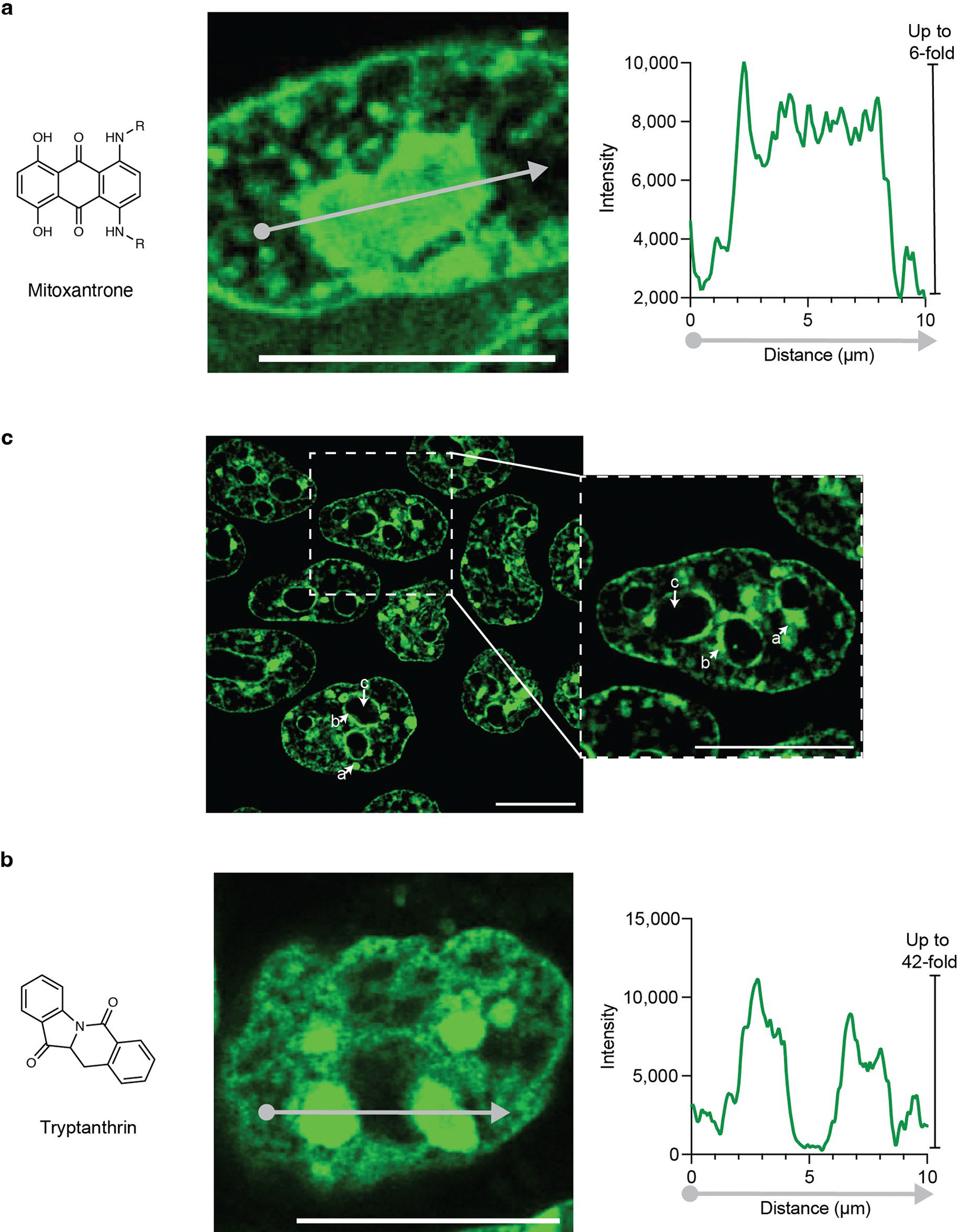
a, Micrograph and line plot showing the signal intensity from mitoxantrone along that indicated gray arrow in HCT-116 cells. b, Mouse embryonic stem cells stained with the DNA dye Hoechst. (a) chromocenter, (b) perinuclear heterochromatin, (c) nucleolus. Zoom (2x). c, Micrograph and line plot showing the signal intensity from tryptanthrin along the indicated gray arrow in mouse embryonic stem cells. Scale: 10 μm. Images were recorded after 1 hour of incubation for tryptanthrin and mitoxantrone, and 10 minutes for hoechst.
Supplementary Material
Acknowledgements
We thank Jesse Platt, Jaime H. Cheah, Christian Soule, Wendy Salmon and Cassandra Rogers for comments and discussion and Andrew Tubelli for graphic art.
Funding:
Supported by NIH GM144283 (R.A.Y), CA155258 (R.A.Y.), NSF PHY2044895 (R.A.Y.). Damon Runyon Cancer Research Foundation Fellowship 2458–22 (H.R.K), NSF Graduate Research Fellowship 1745302 (K.J.O.), MIT Jameel Clinic for Machine Learning in Health and Eric and Wendy Schmidt Center, Broad Institute (P.G.M), Basic Science Research Institute Fund 2021R1A6A1A10042944 (Y.-T.C.) and the National Research Foundation of Korea (NRF) grant funded by the Korea government (MSIT) (2023R1A2C300453411 (Y.-T.C.).
Footnotes
Competing interests:
R.A.Y. is a founder and shareholder of Syros Pharmaceuticals, Camp4 Therapeutics, Omega Therapeutics, Dewpoint Therapeutics and Paratus Sciences, and has consulting or advisory roles at Precede Biosciences and Novo Nordisk. R.B. has consulting or advisory roles at Dewpoint Therapeutics, J&J, Amgen, Outcomes4Me, Immunai, and Firmenich. H.R.K. is a consultant of Dewpoint Therapeutics. The remaining authors declare no competing interests.
Code availability:
Code is available at the following GitHubs:
Machine learning tools: https://github.com/pgmikhael/ChemicalGrammar
In vitro droplet assays: https://github.com/jehenninger/in_vitro_droplet_assay
RDKit Calculations: https://github.com/hrkilgore/rdkit_scripts
PLSR Model: https://github.com/uberholzer/partitioning_PLSR.git
Data availability:
Source and probe partitioning screen data is available at DOI: 10.6084/m9.figshare.23736693 10.6084/m9.figshare.23535258.
Main text references:
- 1.Banani SF, Lee HO, Hyman AA & Rosen MK Biomolecular condensates: Organizers of cellular biochemistry. Nat. Rev. Mol. Cell Biol. 18, 285–285 (2017). [DOI] [PMC free article] [PubMed] [Google Scholar]
- 2.Alberts B et al. Molecular biology of the cell. 7th edn, (W. W. Norton & Company, 2022). [Google Scholar]
- 3.Klein IA et al. Partitioning of cancer therapeutics in nuclear condensates. Science 368, 1386–1392 (2020). [DOI] [PMC free article] [PubMed] [Google Scholar]
- 4.Kilgore HR & Young RA Learning the chemical grammar of biomolecular condensates. Nat. Chem. Biol, 18, 1298–1306 (2022). [DOI] [PMC free article] [PubMed] [Google Scholar]
- 5.Shin Y & Brangwynne CP Liquid phase condensation in cell physiology and disease. Science 357 (2017). [DOI] [PubMed] [Google Scholar]
- 6.Langdon EM & Gladfelter AS A New Lens for RNA Localization: Liquid-Liquid Phase Separation. Annu. Rev. Micrbiol. 72, 255–271 (2018). [DOI] [PubMed] [Google Scholar]
- 7.Lyon AS, Peeples WB & Rosen MK A framework for understanding the functions of biomolecular condensates across scales. Nat. Rev. Mol. Cell Biol. 22, 215–235 (2021). [DOI] [PMC free article] [PubMed] [Google Scholar]
- 8.Alberti S & Hyman AA Biomolecular condensates at the nexus of cellular stress, protein aggregation disease and ageing. Nat. Rev. Mol. Cell Biol. 22, 196–213 (2021). [DOI] [PubMed] [Google Scholar]
- 9.Feric M & Misteli T Phase separation in genome organization across evolution. Trends Cell Biol. 31, 671–685 (2021). [DOI] [PMC free article] [PubMed] [Google Scholar]
- 10.Forman-Kay JD, Ditlev JA, Nosella ML & Lee HO What are the distinguishing features and size requirements of biomolecular condensates and their implications for RNA-containing condensates? RNA 28, 36–47 (2022). [DOI] [PMC free article] [PubMed] [Google Scholar]
- 11.Du M & Chen Zhijian J DNA-induced liquid phase condensation of cGAS activates innate immune signaling. Science 361, 704–709 (2018). [DOI] [PMC free article] [PubMed] [Google Scholar]
- 12.Howard TP & Roberts CWM Partitioning of Chemotherapeutics into Nuclear Condensates; Opening the Door to New Approaches for Drug Development. Mol. Cell 79, 544–545 (2020). [DOI] [PubMed] [Google Scholar]
- 13.Lyons H et al. Functional partitioning of transcriptional regulators by patterned charge blocks. Cell 186, 327–345.e328 (2023). [DOI] [PMC free article] [PubMed] [Google Scholar]
- 14.Sabari BR et al. Coactivator condensation at super-enhancers links phase separation and gene control. Science 361, eaar3958 (2018). [DOI] [PMC free article] [PubMed] [Google Scholar]
- 15.Larson AG et al. Liquid droplet formation by HP1α suggests a role for phase separation in heterochromatin. Nature 547, 236–240 (2017). [DOI] [PMC free article] [PubMed] [Google Scholar]
- 16.Patel A et al. A Liquid-to-Solid Phase Transition of the ALS Protein FUS Accelerated by Disease Mutation. Cell 162, 1066–1077, doi: 10.1016/j.cell.2015.07.047 (2015). [DOI] [PubMed] [Google Scholar]
- 17.Rogers D & Hahn M Extended-Connectivity Fingerprints. J. Chem. Inf. Model. 50, 742–754 (2010). [DOI] [PubMed] [Google Scholar]
- 18.Mater AC & Coote ML Deep Learning in Chemistry. J. Chem. Inf. Model. 59, 2545–2559 (2019). [DOI] [PubMed] [Google Scholar]
- 19.Walters WP & Barzilay R Applications of Deep Learning in Molecule Generation and Molecular Property Prediction. Acc. Chem. Res. 54, 263–270 (2021). [DOI] [PubMed] [Google Scholar]
- 20.Hunter CA & Sanders JKM The nature of π-π interactions. J. Am. Chem. Soc. 112, 5525–5534 (1990). [Google Scholar]
- 21.Thakuria R, Nath NK & Saha BK The Nature and Applications of π–π Interactions: A Perspective. Cryst. Growth Des. 19, 523–528 (2019). [Google Scholar]
- 22.Dougherty DA The Cation−π Interaction. Acc. Chem. Res. 46, 885–893 (2013). [DOI] [PMC free article] [PubMed] [Google Scholar]
- 23.Stewart JA, McCormack JJ & Krakoff IH Clinical and clinical pharmacologic studies of mitoxantrone. Cancer Treat. Rep. 66, 1327–1331 (1982). [PubMed] [Google Scholar]
- 24.Kaur R, Manjal SK, Rawal RK & Kumar K Recent synthetic and medicinal perspectives of tryptanthrin. Bioorg. Med. Chem. 25, 4533–4552 (2017). [DOI] [PubMed] [Google Scholar]
- 25.Wang J et al. A molecular grammar governing the driving forces for phase separation of prion-like RNA binding proteins Cell 174, 688–699.e616 (2018). [DOI] [PMC free article] [PubMed] [Google Scholar]
- 26.Martin EW et al. Valence and patterning of aromatic residues determine the phase behavior of prion-like domains. Science 367, 694–699 (2020). [DOI] [PMC free article] [PubMed] [Google Scholar]
- 27.Choi J-M, Holehouse AS & Pappu RV Physical principles underlying the complex biology of intracellular phase transitions. Annu. Rev. Biophys. 49, 107–133 (2020). [DOI] [PMC free article] [PubMed] [Google Scholar]
- 28.RDKit: Open-Source chemoinformatics (2010).
- 29.Pedregosa F et al. Scikit-learn: Machine Learning in Python. J. Mach. Learn. Res. 12, 2825–2830 (2011). [Google Scholar]
- 30.Mevik B-H & Wehrens R The pls Package: Principal Component and Partial Least Squares Regression in R. Journal of Statistical Software 18, 1 – 23 (2007). [Google Scholar]
- 31.R: A language and environment for statistical computing (R Foundation for Statistical Computing, Vienna, Austria, 2022). [Google Scholar]
- 32.Mehmood T, Liland KH, Snipen L & Sæbø S A review of variable selection methods in Partial Least Squares Regression. Chemometrics and Intelligent Laboratory Systems 118, 62–69 (2012). [Google Scholar]
- 33.Yang K et al. Analyzing Learned Molecular Representations for Property Prediction. J. Chem. Inf. Mod. 59, 3370–3388 (2019). [DOI] [PMC free article] [PubMed] [Google Scholar]
- 34.Jin W, Barzilay R & Jaakkola T Multi-Objective Molecule Generation using Interpretable Substructures. Proc. 37th Int. Conf. Mach. Learn. (2020). [Google Scholar]
- 35.Schindelin J et al. Fiji: an open-source platform for biological-image analysis. Nature Methods 9, 676–682 (2012). [DOI] [PMC free article] [PubMed] [Google Scholar]
Associated Data
This section collects any data citations, data availability statements, or supplementary materials included in this article.
Supplementary Materials
Data Availability Statement
Source and probe partitioning screen data is available at DOI: 10.6084/m9.figshare.23736693 10.6084/m9.figshare.23535258.