Haplotype Fine Mapping by Evolutionary Trees

Summary

To refine the location of a disease gene within the bounds provided by linkage analysis, many scientists use the pattern of linkage disequilibrium between the disease allele and alleles at nearby markers. We describe a method that seeks to refine location by analysis of “disease” and “normal” haplotypes, thereby using multivariate information about linkage disequilibrium. Under the assumption that the disease mutation occurs in a specific gap between adjacent markers, the method first combines parsimony and likelihood to build an evolutionary tree of disease haplotypes, with each node (haplotype) separated, by a single mutational or recombinational step, from its parent. If required, latent nodes (unobserved haplotypes) are incorporated to complete the tree. Once the tree is built, its likelihood is computed from probabilities of mutation and recombination. When each gap between adjacent markers is evaluated in this fashion and these results are combined with prior information, they yield a posterior probability distribution to guide the search for the disease mutation. We show, by evolutionary simulations, that an implementation of these methods, called “FineMap,” yields substantial refinement and excellent coverage for the true location of the disease mutation. Moreover, by analysis of hereditary hemochromatosis haplotypes, we show that FineMap can be robust to genetic heterogeneity.

Introduction

Demonstrating linkage between a disease gene and a marker is only one step on the often long road to cloning the gene. After demonstration of linkage, further recombinant mapping usually can refine the critical region, especially for simple genetic disorders. Rarely, however, has recombinant mapping enjoyed much success once the critical region has been reduced to one or two megabases. This bottleneck is caused by the improbability that recombinants will be observed in extant family material (Boehnke 1994). For these cases, researchers have turned to other methodologies. For simple genetic disorders, one successful approach has been to infer a critical subinterval, from the fact that ancestral recombinant breaks can produce a predictable pattern of linkage disequilibrium between the disease gene and a set of markers spanning the critical region (Kerem et al. 1989; Hästbacka et al. 1992, 1994).

Indeed, the analysis of linkage disequilibrium in various guises is now widely used for fine mapping and has enjoyed much success (for review, see Devlin and Risch 1995; Jorde 1995; de la Chapelle and Wright 1998). Yet there remain open questions about how to use optimally the information from linkage disequilibrium. As far as we are aware, three general analyses are applied for linkage-disequilibrium mapping: simple disequilibrium mapping, by which the pattern of pairwise disequilibrium between the disease gene and each of a set of markers is examined (e.g., see Kerem et al. 1989; Feder et al. 1996); likelihood-based analyses, which use the same information (e.g., see Hästbacka et al. 1992; Kaplan et al. 1995; Devlin et al. 1996); and haplotype fine mapping, which is the focus of this report.

Devlin and Risch (1995) examine the properties of simple disequilibrium mapping, providing theoretical support for the empirical success of this approach. Likelihood-based methods that use the same information are complementary and more-rigorous approaches to inference. When the information from multiple markers spanning the critical region is to be integrated, both methods rely on a multinomial distribution of recombinant breaks in intervals between markers. When only a small number of recombinants are available for sampling—as will often be the case for small critical regions and relatively recent disease mutations—the distribution is inaccurately estimated, and information from a sample of disease chromosomes will be unreliable (Devlin et al. 1996). Other methods, which rely on haplotype information, may be more useful in these settings.

Unlike pairwise disequilibrium methods, methods using haplotypes to fine-map disease genes are relatively undeveloped. Most researchers use approaches that are analogous to simple disequilibrium mapping in that they evaluate the pattern of haplotype-sharing without formal statistical analysis. Recently, both McPeek and Strahs (1999) and Service et al. (1999) have provided statistically based methods. In this article we propose a different statistical method for haplotype fine mapping and make available a computer program (FineMap) to implement it. The data for FineMap are a sample of disease and normal chromosomes, each chromosome in which is typed for a set of polymorphic genetic markers.

With the assumptions (a) that the disease mutation falls within a specified gap between adjacent markers and (b) that a single ancestral mutation gave rise to all disease haplotypes (the homogeneous case), the first stage of the analysis combines parsimony and likelihood, to build an evolutionary tree of disease haplotypes with each node (haplotype) separated, by a single mutational or recombinational step, from its parental node. The guiding principle for connecting nodes is that the disease mutation must be preserved in the assumed gap for all haplotypes. If more than one mutational or recombinational step is required to connect some nodes, latent nodes (unobserved haplotypes) are incorporated to complete the tree. An illustration of this process is given in figure 1a. Once the tree is built, its likelihood can be calculated on the basis of the probability model for mutations and recombinations as well as on the basis of prior information about the shape of the tree. On the basis of the likelihood model, each gap is assigned a posterior probability that the disease mutation is located within the interval.

Figure 1.

Homologous portions of a chromosome. The colored blocks represent adjacent markers, and matching colors represent matching alleles. a, Illustration of how, under the assumption that the disease mutation lies in gap 4, between markers 4 and 5, observed haplotypes A–E might be arranged with A as the root. In the tree, A→D and L1→E are unambiguous recombinations, whereas the other edges could be caused by either recombination or mutation. Notice that, although haplotypes A and E are similar, they cannot be directly connected by a single edge. It appears that a haplotype is missing from the sample (or the population). Thus a latent haplotype (L1) is required for completion of the tree. The topology is approximately star shaped, with most haplotypes directly connected to the root, as would be expected from evolutionary theory for rapidly growing populations. b, Same scenario under the assumption that three more haplotypes (F–H) are observed. Of haplotypes A–E, F is most similar to D. To connect this pair, two latent haplotypes are required. Consequently, when the haplotypes are fit into a single tree, the tree is spindly rather than star shaped. If, however, two trees are fit to these data, then haplotypes A–E and F–H will split into separate clusters.

For the heterogeneous case, only subsets of haplotypes can be organized into coherent evolutionary trees, and the number of such clusters is unknown. For each disease location and specified number of clusters, the algorithm organizes the data into (approximately) homogeneous clusters and fits separate trees to each cluster (fig. 1). The algorithm now compares the fit of the data to models with varying numbers of clusters. On the basis of a diagnostic, the data analyst chooses how many clusters to fit, and then inference will be based on the biggest cluster only.

Although our proposed method is likelihood based, it does not attempt to evaluate the full likelihood. We deliberately chose simplicity, for several reasons. First, we believe that the results of this method are easy for the user to interpret. Second, because of its simplicity, our method requires only a simple assumption regarding the evolutionary process. Third, our method is very flexible and should be extensible (with modifications) to settings more complex than those described herein. We believe that such flexibility will be critical for haplotype fine mapping of complex disease genes, for which disease chromosomes may not be identifiable and which are linked to a particular region in only a fraction of cases. Our method is designed to fine-map a gene in its critical region, on the basis of the information from haplotype-sharing; if a researcher were to attempt to fine-map a nonexistent gene, the method's behavior would be unpredictable.

In our section on “The Probability Model,” we develop the probability model underlying our approach to fine mapping. After the overview are descriptions of each component of the probability model, such as the recombination likelihood and the mutation likelihood. In the next section, “Inference about d,” we describe methods of inference that are based on the previously developed probability model. Inference for a single ancestral haplotype is presented, then a sketch of the tree-building algorithm (full details are in Appendix B), and, finally, we revisit inference while outlining our treatment of multiple ancestral haplotypes. In the third section, “FineMap Performance,” we describe the performance of the method, on the basis of evolutionary simulations, and the analysis of some data on hereditary hemochromatosis (HH) haplotypes. Readers may wish to look ahead to this last subsection, which makes the methodological developments concrete by the analysis of HH data.

The Probability Model

Let the sample space be the population of disease haplotypes consisting of ordered markers labeled from “1” to “L.” We index the gaps between adjacent markers from left (proximal) to right (distal) on a haplotype, with d being the gap containing the mutation and 𝒟 being the set of gaps under consideration. Let 𝒯 be the space of rooted-tree topologies, which describe the ancestor-descendant relationships between haplotypes, and let τ represent a particular topology. The parameter of interest is λ=(d,τ). Let Y be a random sample from the sample space, and let Y^′=(S₀,…,S_n) be the unique haplotypes in Y, with evolutionary time advancing from the root S₀ and radiating outward through the branches of the tree.

Overview

Given the topology of the directed tree τ and a disease located in gap d, the likelihood of observing Y reduces, by the Markovian property of such trees, to

where the product is taken over all edges in the graph. In the spirit of parsimony, a simple likelihood is obtained by assuming that each edge represents a single evolutionary change. Thus T∣S means that T is a descendant of S via either a single mutation or recombination. Through this assumption time drops out of the likelihood, as described below. For any empirical fine-mapping effort, this single-change assumption is satisfied by imputing any missing nodes. Latent nodes are restricted to those haplotypes that differ from their predecessor by a single marker. This restriction is imposed to control the influence of latent haplotypes on inference. Given a set of observed and latent haplotypes, the likelihood of the tree is computed as the product of edges (see eq. [1]), without regard for whether the nodes are observed or latent.

A priori, it is unclear whether an edge represents a mutation or a recombination, so we average over the uncertainty between the two possibilities to form a mixed likelihood. Let P(mut∣mut or rec) and P(rec∣mut or rec) be the relative probabilities that a mutation or a recombination occurred, given that, at most, a single mutation or recombination occurred. Then the edge likelihood is P_λ(T∣S)=P_λ(T∣S,mut)P(mut∣mut or rec)+P_λ(T∣S,rec)P(rec∣mut or rec).If S and T differ at more than one locus, then P_λ(T∣S,mut) is 0, and it is clear that a recombinational event occurred. The edge likelihood then simplifies to P_λ(T∣S)=P_λ(T∣S,rec)P(rec∣mut or rec). If S and T differ at exactly one locus, then both terms contribute to the likelihood.

To compute the relative probability of a single mutation, P(mut∣mut or rec), we require an estimate of the probability of observing either exactly one mutational (A) or one recombinational event (B). Then it follows that P(mut∣mut or rec)=A/(A+B). Let γ_k be the probability of a mutation at locus k. The probability of one mutation during a given meiosis is then A=Σ_kγ_kΠ_i≠k(1-γ_i). Analogously, let θ_j be the probability of a recombination in gap j. The probability of recombination during a given meiosis is then B=Σ_jθ_jΠ_i≠j(1-θ_i).

There is little information available from which to model the root probability; P_λ(S₀ is root) is estimated by the proportion of the haplotype S₀ in Y, given that older disease haplotypes are expected to be more numerous than their younger descendants (Donnelly 1986). It will become clear shortly that this estimate has little impact on the likelihood.

Recombination Likelihood

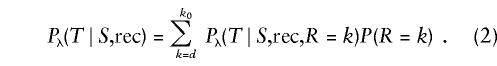
Suppose that S and T appear to be related through a recombination and that the two haplotypes are identical by state (IBS) proximal to gap k₀ and differ distal to gap k₀. (We define “IBS” here as any identical pair of haplotypes regardless of descent relations, following Lange [1997; Elandt-Johnson 1971], and define “IBS*” to mean that, although the haplotypes are identical, a portion, at most, of the haplotype is identical by descent [IBD].) Let R be the gap number of the point of recombination. The point of recombination could be anywhere between the disease location d and k₀; hence the likelihood for a recombination edge of the evolutionary-tree topology is

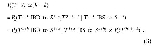
Let S^m:n be the fragment of S spanned by markers m,m+1,…,n. Focus on the first term on the right side of the equation above. If T is directly connected to S and the edge is determined by a recombinant break in gap k, then T^1:k must be IBD to S^1:k and T^(k+1):L is a partial haplotype obtained via recombination. Therefore,

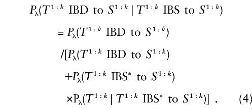
By an application of Bayes's theorem,

To complete the likelihood, we require a model for P_λ(T^(k+1):L), the probability of obtaining a given haplotype such as T^(k+1):L through the process of recombination. Our approach is described below, under “Nonparametric Haplotype Probabilities.”

In equation (2), by summing over recombinant location from k=d,…,k₀, our model allows for cryptic recombinations—that is, recombinations that extend from L over to d even if S and T are IBS proximal to k₀. Although probabilistically correct, this likelihood requires a good model for P_λ(T^k:L). Unless a very large number of normal haplotypes have been sampled, accurate estimates of haplotype frequencies are unlikely. To compensate, we replace equation (2) with the noncryptic recombinant model, which presumes the occurrence of the shortest possible recombination consistent with the data: P_λ(T∣S,rec)=P_λ(T∣S,rec,R=k₀)P(R=k₀). This likelihood is more conservative than equation (2), because it underestimates the probability of the recombination and hence provides a somewhat broader credible interval for location of the disease mutation.

Throughout the discussion above, we assume that a single recombination has occurred. Implicitly, we write P(R=k) to mean P(R=k∣no. rec=1). If we let b and b_k denote the probability of a recombination in the entire interval and in the kth gap, respectively, then

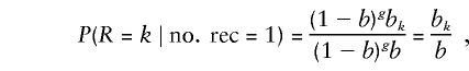where g+1, the number of generations until S recombines to form T, conveniently cancels out of the equation.

In practice, other terms in the likelihood must be specified. For example, we might assume, a priori, that P_λ(T^1:k IBD to S^1:k)=P_λ(T^1:k IBS^* to S^1:k)= 1/2. This noninformative prior favors neither of the hypotheses. Making the IBD hypothesis less probable has the effect of diminishing the chances of falsely connecting haplotypes in an evolutionary tree. Thus, for a given problem, we might choose a prior favoring either hypothesis, using this term as a tuning parameter. The quantity P_λ(T^1:k∣T^1:k IBS^* to S^1:k) appearing in equation (4) can most easily be computed empirically as the frequency of T^(1:k) in a reference sample of haplotypes, as described below under “Nonparametric Haplotype Probabilities.”

Another difficulty with practical implementation is that it can be impossible to estimate recombination fractions between markers separated by relatively small physical distances. In this instance, it seems reasonable to assume that θ_k/θ is proportional to the length of gap k, and, because interest lies in small critical regions, to take 1 cM = 1 Mb. Rough estimates of physical distance separating markers are usually available for fine-mapping efforts, and these estimates should be sufficient (see below, under “HFE and HH”).

Mutation Likelihood

There are many kinds of genetic markers that could prove useful for fine mapping. Of these, the most commonly used markers are short tandem repeats (STRs). Arguably, in the near future, single-nucleotide polymorphism (SNP) markers may be favored. The latter are believed to have a very small probability of mutation, on the order of 10^-6–10^-8. Thus, mutation probabilities for SNPs will have very little influence on the likelihood, and most changes in SNP-based haplotypes will be because of recombination. STRs are a different matter; their mutation rates appear to vary between 10^-2 and 10^-4 (for polymorphic repeats). Thus, this section focuses on the case of STR markers, although the method (and FineMap) accommodate any kind of genetic marker.

If two haplotypes, S and T, in the evolutionary tree are related through a mutation, then the two haplotypes must differ at exactly one marker position. In this case, time drops out of the likelihood, for the same reason that it drops out of the recombinant likelihood. Let M be the marker position at which they differ, let L be the length of the haplotype, and let S^(-m) denote haplotype S excluding position m.

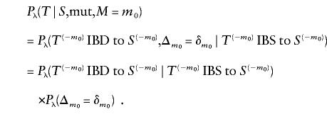
Define to be the size of the mutation change between S and T at marker m (i.e., the difference between the number of repeating units of the STR), and suppose that Δ_m∼μ_m for some probability distribution μ_m. If S and T differ at position M=m₀, then the likelihood for a mutation edge of the evolutionary tree topology is P_λ(T∣S,mut)=P_λ(T∣S,mut,M=m₀)P(M=m₀). Focus on the first factor on the right side of the equation above. If T is connected by an edge to S and the edge is determined by a mutation at position m₀, then T^(-m₀) must be IBD to S^(-m₀), and T^m₀:m₀ is obtained through a mutation of size δ_m0. Therefore,

In practice, mutation rates for the marker loci and the distribution of mutational changes are required. Mutation rates and the distribution of size changes for STRs can be estimated directly from population data (Chakraborty et al. 1997; Rannala and Slatkin 1998), although it is unclear how effective these estimation methods are for individual loci. In any case, the method and FineMap can readily accommodate differential mutation rates and sizes of mutations, however they are derived.

One simple solution is to assume that mutation rates are constant across loci and to glean both the mutation rate and the distribution of mutational changes from the literature. Weber and Wong's empirical study (1993) suggests γ_m .001 with one-step mutations at rate = 10/11. Alternatively, one might allow mutation rates to vary across loci by estimating locus-specific rates while keeping a simple model for mutation size. We present such an analysis in Appendix A and apply these rates to the HH data (see below, under “HFE and HH”).

Nonparametric Haplotype Probabilities

Throughout this section, it is assumed that a sample of haplotypes is available from which the frequency of partial haplotypes may be empirically estimated. In equations (3) and (4) estimates of terms such as P_λ(T^1:m) are required. If a large reference sample of haplotypes is available, this quantity would ideally be approximated by the frequency of T^1:m in the sample. However, even for a large reference database, the observed frequency of the partial haplotype in the sample may be 0. Consequently, we approximate the required probability when necessary, as described below.

The probability of observing the partial haplotype [x₁x₂⋅⋅⋅x_m] can be written as

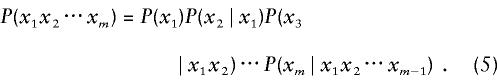The simplest approach to estimating this quantity assumes independence between the markers and estimates equation (5) by the product of allele frequencies. Another simple approach assumes a first-order Markov model; however, the Markov model may not be very accurate, because dependencies can extend much farther than neighboring markers. To account for the positive dependencies between alleles, we can base the conditional probabilities on the highest possible level of “haplotype dependence” in the reference database. Suppose that the longest observed haplotype matching [x₁x₂⋅⋅⋅x_j] and including x_j is [x_j-2x_j-1x_j]. Then we define

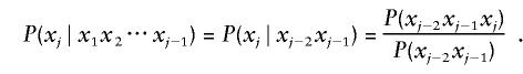When the partial haplotype of interest is observed in the database, this estimator is simply the observed frequency of the haplotype.

In general, the haplotype database used in this analysis would be derived from “normal” chromosomes. If the reference database consists of multilocus genotypes rather than haplotypes, then gene-counting approaches, such as those developed by Hawley and Kidd (1995) and Xie and Ott (1993), could be used to obtain estimates of haplotype frequencies. To avoid haplotype frequency estimates of 0, a modified version of the method described above could be implemented to obtain partial haplotype frequencies.

Prior Distributions and Penalized Likelihood

We note that any valid prior information can be incorporated into the probability model (and into FineMap). Here we describe priors that are automatically implemented by FineMap on the basis of prior information about d and τ. Prior information can also be incorporated into a likelihood analysis via a penalty function.

Priors

Unless the markers were specifically developed with a particular gene in mind, the disease mutation is more likely to fall within a larger gap than in a smaller one. Thus, with no extra prior information, a simple but sensible choice for the prior over the possible disease locations π_𝒟 places mass in the dth gap, proportional to the relative physical length of the dth gap.

As for the prior over the tree space π_𝒯, we note that many human populations have experienced exponential growth during the past several hundred generations, and such growth has the impact of creating approximately star-shaped trees in which much of the branching occurs at or near the root (Slatkin 1996). To incorporate this feature into the likelihood, we formulate a prior for tree topologies that favors trees that are approximately star shaped. To formalize this idea, given a tree topology τ, let Z_j be the number of extra edges required to connect S_j to the root. This value is 0 if S_j is directly connected to the root; otherwise, it is equal to the number of nodes separating S_j from the root. The total number of extra edges in the tree isC=Σⁿ_j=1Z_j. C is assumed to follow a Poisson (nφ) distribution, in which φ can be interpreted as the expected number of extra edges required to connect an observed haplotype to the root, or the mean depth of the tree topology. Set π_T(τ)=P(C(τ)∣φ). Provided that a fairly small value for φ is chosen, this prior favors trees that are approximately star shaped. For example, for φ=1 this prior gives equal weight to paths with 0 or 1 extra edges and considerably less weight to trees with paths having an average of ⩾2 extra edges. We have found φ=1 (2) to be a sensible choice for mutations of about ∼100 (∼200) generations old.

Penalized likelihood

For a given gap location d, if we perform a direct maximization of the likelihood to find , we ignore the fact that the data most likely are generated by evolutionary processes favoring star-shaped trees, as noted above. We can improve our model selection by performing a penalized likelihood analysis (see Good and Gaskins 1971), in which the optimal tree maximizes the penalized log likelihood, logP(Y∣d,τ)-penalty(λ). In the tradition of penalized likelihood, the purpose of the penalty is to down-weight trees that are overly complex, with branching occurring far away from the root. A natural choice for the penalty function is -logπ_𝒯(τ), as it has the desired properties.

It is more convenient to work with the negative of the penalized log-likelihood, because log probabilities are negative. This quantity can be interpreted as the weight of, or the cost to explain, the observed haplotypes in the topology. To summarize, for a given subset of haplotypes, 𝒮, the objective is to find τ to minimize the quantity w_d(τ)=-logP(𝒮∣d,τ)-logπ_𝒯(τ). Because of the choice of the penalty function, this function is also the negative-log joint posterior distribution of (d,τ).

Inference about d

Single Ancestral Haplotype

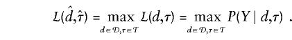
We wish to determine which gap between adjacent markers actually contains the disease mutation. If all that is desired is a point estimate for its location, then, given the probability model, we can calculate the maximum-likelihood estimate by finding , such that

Alternatively, we could consider a Bayesian analysis that is based on the marginal posterior distribution of d, rather than on the likelihood:

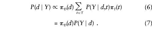The random variable d takes on a finite set of values; thus, the proportionality constant can be computed directly. In the Bayesian analysis, a natural point estimator for d is the mode of the posterior distribution of d. Likewise, a natural interval estimate for d is a γ%-credible interval, which is the Bayesian analogue to a confidence interval and is the smallest continuous interval containing ⩾γ% of the posterior probability (Lee 1989).

In practice, direct computation of the marginal posterior is infeasible, because we cannot truly perform the summation in expression (6). Unlike the tree spaces encountered in certain phylogeny problems, the possible presence of latent nodes in the tree topologies creates an infinite number of trees to consider. A convenient approximation to P(Y∣d) in expression (7) for our purposes is , where minimizes w_d(τ). This is simply the largest term of the sum in expression (6). Bounds on the approximation can be computed by following the approach of Liu et al. (1999).

Maximization over the Tree Space

Inferences based on d, whether maximum-likelihood estimates or posterior distributions, ultimately rely on maximizing some given function over 𝒯. However, this task is quite difficult, because 𝒯 has infinite cardinality and is without an algorithmically useful mathematical definition, which makes it difficult to search in a systematic way. A way around this problem is to use heuristics to construct a tree that lies within a small neighborhood of the optimal tree in 𝒯 and to use the constructed tree as an approximation to the optimal tree. Our chosen heuristics favor trees with fewer latent nodes, because fewer latent nodes implies fewer edges to multiply together when the likelihood is computed. When we do impute latent nodes between ancestral and descendant haplotypes, we choose them to maximize the total probability of edges from the ancestor to the descendant.

Suppose that we are given a disease location d. The idea is to build trees iteratively by joining larger and larger clusters of haplotypes. Clades, the smallest clusters of haplotypes where each edge represents a single-locus change, should join first. We want to merge clusters that “best” merge together, meaning that, at a given iterative step, the two haplotype clusters with the highest probability path between them should be merged together. We stop when only a single cluster remains. The details of the tree-building algorithm can be found in Appendix B.

Multiple Ancestral Haplotypes

There are several scenarios under which the observed haplotypes cannot be organized into a single evolutionary tree: (i) the disease mutation evolved from a single ancestral haplotype, but the early history of the tree has been lost; (ii) the disease mutation arose more than once in the population, each time on a different ancestral haplotype; (iii) more than one type of disease mutation is present in the gene under study; and (iv) some diseased individuals do not have a mutation in the gene under study. In this subsection, we lay out an approach to treating such heterogeneous data. This methodology requires that at least a cluster of disease haplotypes has evolved from a common ancestral chromosome. The objective is to find this cluster, 𝒮^*, and to analyze it as described in the previous subsection. Clearly, the effectiveness of the analysis increases as the fraction of the sample descending from a common ancestor increases.

The method of building trees described in the previous section can be used easily to find appropriate clusters of haplotypes, because, given a fixed disease location d, we can choose when to stop the iterative clustering process by conditioning on the existence of a weakly connected components. These subsets may be found for each a-and-d value. Define 𝒮_ad to be the largest of these subsets of haplotypes, given a and d. We focus our interest only on this largest subset, since it is unlikely that a sample of observed haplotypes will be large enough to yield useful information concerning the smaller remaining clusters of haplotypes.

To select our desired subset 𝒮^* from {𝒮_ad:a⩾1,1⩽d⩽L}, whose elements are likely to be of varying sizes, we need a size-independent metric. Let be the number of unique observed haplotypes in 𝒮_ad. Then one such metric is , where τ_ad is the evolutionary tree for 𝒮_ad found during the clustering process. W_ad may be interpreted as the average weight of a path from the root to an observed haplotype.

The following outlines our algorithm to find the best subset of data:

• 1. Fix a, and, for each disease location d, find 𝒮_ad.
• 2. For each a, find d=d^*(a) that minimizes W_ad as a function of d.
• 3. Plot W_ad^*(a) as a function of a.
• 4. Choose a=a^* as the point that gives a dramatic decrease in W_ad^*(a).
• 5. Declare 𝒮^*=𝒮_a^*d^* and use it for inference as described above, under the heading “Single Ancestral Haplotype.”

The metric W_ad^*(a) is nonincreasing in a, because it is always possible to obtain a reduction in the overall average path weight by removing the heaviest path weight from the tree topology. For this reason, we look for a dramatic drop in the criterion, rather than aiming for the absolute minimum. This approach is akin to a model-selection criterion for the number of principal components and for the number of dimensions in multidimensional scaling (Jobson 1992). Because step 4 is not based on a strictly objective criterion, the choice of a^* is not determined automatically (i.e., the user of FineMap must make this choice).

Note that a^* may be 2, even when the smaller subset of haplotypes does not share a common evolutionary history. This observation follows because the metric W_ad^*(a) depends only on the largest subset of haplotypes. If this subset is correctly selected in the first split, it is unlikely to change very much as a grows.

Choice of the appropriate subset of haplotypes exerts a great deal of influence on the analysis. Thus, we suggest some additional informal diagnostics. Define two observed haplotypes as adjacent if they are either directly connected by an edge or connected via a series of edges defined by one or more latent nodes. Define the adjacent path weight as the sum of the weights corresponding to the edges connecting two adjacent haplotypes. The key indicators of a poor tree are (i) an unbalanced (i.e., not star-shaped) tree, (ii) heavy paths with multiple latent nodes between adjacent haplotypes, and (iii) only small shared segments between adjacent haplotypes. In general, if one is in doubt, the analysis should be performed without the haplotypes that are difficult to connect to the tree (as defined by ii and iii above). A more formal implementation of this idea would involve performing a jackknife resampling approach to locate haplotypes of high influence (Davison and Hinkley 1997). In our experience, choosing too large a value for a^* tends to increase the size of the credible interval. Within reasonable limits, it will not bias the results in any other manner. If excluding a haplotype changes the results dramatically, the investigator should interpret the results with great caution.

FineMap Performance

Simulations

Methods

The evolutionary program mimicked features of natural populations as closely as possible by using direct simulation methods. Diploid individuals paired at random in their generation, mated, and produced a random number of children. The expected number of progeny per couple was determined by an exponential growth rate, and the variance in progeny number was binomial (i.e., Fisher-Wright model [Kingman 1982]). Each population was founded by 1,000 individuals and remained at that size for 50 generations. This initialization, together with small population growth in early generations, generated random linkage disequilibrium among alleles on normal chromosomes. After 50 generations, a disease mutation was introduced on one chromosome and the population grew exponentially for 100 or 200 generations, to a final size of 50,000 individuals. If the disease mutation was lost at any generation, or if its relative frequency became too common (>.015), the simulation was reinitiated.

Sixteen STR markers were simulated, covering a 2-Mb critical region, with spacings (in Mb) between markers as follows: m₁ – .25 – m₂ – .25 – m₃ – .011 – m₄ – .011 – m₅ – .011 – m₆ – .011 – m₇ – .011 – m₈ – .011 – m₉ – .011 – m₁₀ – .011 – m₁₁ – .011 – m₁₂ – .011 – m₁₃ – .011 – m₁₄ – .25 – m₁₅ – .25 – m₁₆. This uneven distribution yields two views of FineMap's performance. When all the markers are taken together, FineMap shows the power of haplotypes to refine a fairly large critical region. Alternatively, imagine that the outer, more–widely spaced markers were excluded by linkage analysis. In this case, the simulations give a conservative view of the information available from an evenly spaced grid of markers plus additional, external markers that help to determine recombinants. (In fact, we recommend the inclusion of proximate markers in the analysis, even if the analysis will eliminate them, because they contribute substantial information regarding the origins of haplotypes. An option in FineMap allows the user to designate excluded regions.)

The median number of repeats per marker initially was 50; the initial distribution was roughly bell shaped, with a range of 47–53 and 80% heterozygosity. To produce the founder population, alleles were randomly assigned for each of the 16 markers, to produce a chromosome, and chromosomes were randomly assigned to individuals. We took μ to be a unit-shifted geometric distribution, with Δ_m-1∼geometric (10/11), and took M to have a discrete uniform distribution on {1,…,L}. There were no restrictions on size changes. The mutation rate was .001. The recombination process was a no-interference Poisson model based on the assumption that 1 cM = 1 Mb.

Populations were generated for each of four conditions: for designs I and III, the disease mutation was located in the middle of the critical interval (gap 8); for designs II and IV, the disease mutation was proximal (gap 4). The disease allele occurred 100 (designs I and II) or 200 generations (designs III and IV) generations in the past. From each population, a random sample of 100 disease and normal chromosomes were chosen for analysis.

Results

Simulation results suggest that FineMap's posterior distribution is an excellent guide for the localization of the disease mutation. In fact, FineMap's coverage always exceeded the nominal coverage (table 1). The results also show substantial refinement of the localization of the disease mutation, with greater refinement for older and more–centrally located mutations (table 1).

Table 1.

Achieved Coverage and Length of the Credible Interval for Evolutionary Simulations

	Nominal Coverage (× 105 bp)
Setting	.90	.95	.99
Ia:
Coverage	.970	.985	1.000
Length	5.140	5.350	5.880
IIb:
Coverage	.980	.990	.995
Length	6.420	6.680	7.290
IIIc:
Coverage	.965	.975	.990
Length	4.020	4.190	4.700
IVd:
Coverage	.980	.985	.995
Length	5.570	5.840	6.520

^aDisease mutation arose 100 generations before present (GBP), in the center of the critical region (gap 9 of 17 gaps).

^bMutation arose 100 GBP, in gap 5.

^cMutation arose 200 GBP, in gap 9.

^dMutation arose 200 GBP, in gap 5.

For the simulation analyses, we used φ=1.0 (2.0) for the Poisson prior on tree topologies. These priors agree roughly with the average tree obtained from simulation results: when trees were built conditional on the mutation being placed in its true location, the average depth (C/n) was 0.96, 0.94, 1.75, and 1.73, for 100 generations symmetric, 100 generations asymmetric, 200 generations symmetric, and 200 generations asymmetric, respectively. To evaluate the impact of a range of reasonable values for φ, we evaluated the design I simulations with φ of 0.2, 0.5, and 2.0 (table 2). Clearly, coverage results were relatively insensitive to plausible choices of φ.

Table 2.

Achieved Coverage and Length of Interval for Design I Simulations (Table 1) for Different Priors on Tree Topologies (i.e., Different φ)

	Nominal Coverage (× 105 bp)
φ	.90	.95	.99
.2:
Coverage	.98	.98	1.000
Length	5.03	5.25	5.710
.5:
Coverage	.98	.99	1.000
Length	5.05	5.26	5.780
2.0:
Coverage	.95	.98	.995
Length	5.14	5.46	6.130

For the simulation analyses we used the true mutation model, with mutation rate .001. To evaluate the impact of improper choice of mutation rate, we reanalyzed the design I simulations with a 10-fold-lower mutation rate. Misconstruing the mutation rate had only a minor impact on the analysis.

HFE and HH

HH, which occurs in ∼1/300 Europeans, is a recessively inherited disease resulting from imbalanced iron metabolism. Approximately 90% of cases are caused by a single mutation, in HFE (Feder et al. 1996), that maps to the HLA region on chromosome 6p. To evaluate the effectiveness of linkage disequilibrium in fine mapping of HFE, Thomas et al. (1998) analyzed 43 STR loci from 101 patients of European ancestry who were affected by HH and from 64 Centre d'Étude du Polymorphisme Humain (CEPH) controls, all grandparents of European ancestry. CEPH control chromosomes were phased by genotyping of additional individuals from the parental generation. Only a portion (n=20) of the patients with HH were phased, because the authors' analysis did not require haplotypes. Instead, the authors used the phased chromosomes to identify the ancestral haplotype on which the predominant mutation arose and then used an algorithm based on the transition from homozygosity to heterozygosity to infer ancestral recombinant breaks.

On the basis of these data, we present a worked example to make the development of FineMap concrete. Our analyses use only phased chromosomes derived from two sources: all disease and normal chromosomes presented by Thomas et al. (1998) and the small set of eight chromosomes from individuals with disease that are presented by Feder et al. (1996, table 1). The latter set does not carry the predominant mutation in HFE. Using the authors' map of the HFE critical region, we select 14 contiguous markers from D6S2243 (proximal) to D6S2234 (distal) for analysis. This limited set of markers allows us to phase more disease chromosomes, because they are completely homozygous across the region or are heterozygous at only one marker. The final count of disease chromosomes is 133 (one chromosome being eliminated because of presumed overlap between the Feder et al. and Thomas et al. data sets); the count of normal chromosomes is 128.

Analysis of a homogeneous subset

To keep the initial presentation simple, we analyze a homogeneous subset of disease haplotypes obtained by excluding all haplotypes carrying the 103 allele at D6S2240 (this will be justified shortly). Of the disease haplotypes, 39 are unique. Elimination of those bearing the 103 allele at D6S2240 reduces the number of unique haplotypes to 31. Placing the disease mutation in its true location of gap 8, between D6S2238 and D6S2239, FineMap builds a largely star-shaped tree (fig. 2) consistent with that expected from evolutionary theory for a recent mutation and a rapidly growing population (Slatkin 1996). To build the tree, connecting nodes by one-step changes requires five latents (fig. 3, latents end-labeled by “L”). The color of the haplotypes depicted in figure 3 indicates the differences between haplotypes connected by an edge. Exactly the same tree is built when the disease mutation is placed in gap 9, whereas more-spindly (less star-shaped) trees are required for all other locations for the disease mutation. When the likelihoods for these trees are evaluated and combined with sensible prior information as described previously, almost all probability for location is focused on two gaps, 8 and 9.

Figure 2.

Tree structure for a homogeneous subset of 31 unique HH haplotypes. Circles signify the five inferred, latent haplotypes.

Figure 3.

Observed and latent haplotypes corresponding to figure 2. “ANC” denotes the inferred most recent ancestor, “Weight” denotes the negative log likelihood of the edge connecting the haplotype to ANC, and “[L]” denotes a latent haplotype. The portion of the haplotype that differs from ANC is color-coded green for single-marker differences and red for differences occurring in blocks.

Analysis of the full sample

Approximately 90% of all HH cases can be attributed to an HFE mutation (Feder et al. 1996). Thus, a sample of HH haplotypes is expected to be somewhat heterogeneous. Even so, we supplement the data from Thomas et al. (1998) with an additional eight haplotypes known not to carry the predominant HFE mutation, thereby ensuring heterogeneity and, presumably, raising the difficulty of the analysis.

FineMap's approach to heterogeneity is to find a homogeneous subset of the haplotypes, for further analysis. To find such a subset for the HH data, we applied the algorithm described in our section on “Multiple Ancestral Haplotypes” (table 3). From those results, we chose a=2 and based our inferences on 𝒮^*=𝒮_2,7, the best subset for a=2. These haplotypes match the set of 31 distinct haplotypes that defined our homogeneous subset presented in figures 2 and 3. Remarkably, the eight excluded haplotypes are precisely of the form of the eight supplementary haplotypes obtained from Feder et al. (1996), which do not carry the predominant HFE mutation. Contrast figures 2 and 4, which display, for the selected subset and the entire set of haplotypes, respectively, the best topologies found for d=8. From the spindly nature of the tree in figure 4, it is clear that the excluded haplotypes do not share a common evolutionary history with the subset of 31 haplotypes: the haplotypes labeled 37–57 in figure 4 constitute the set of 8 excluded haplotypes along with the associated latent haplotypes required in order to connect these haplotypes to the rest of the tree (fig. 5). With the exception of this extremely lengthy clade, however, the trees depicted in figures 2 and 4 share a nearly identical structure.

Table 3.

Weight Metric for Differing Subsets of Haplotypes^[Note]

a	Wad*(a)	Drop
1	9.41
2	7.87	1.54
3	7.39	.48
4	6.61	.78

Note.—a indexes the number of subsets of haplotypes; W_ad^*(a) is the value of the metric for the largest of the a subsets.

Figure 4.

Tree structure for the entire set of 39 unique HH haplotypes, plus latents (circles).

Figure 5.

Twenty observed and latent haplotypes corresponding to figure 4 but not reported in figure 3. Combining the observed haplotypes depicted here and in figure 3 yields the entire sample of haplotypes.

Substantial haplotype sharing among disease chromosomes makes it apparent that the predominant HFE mutation is of recent origin. In fact, Thomas et al. (1998) estimate its age at slightly less than 100 generations. For these reasons, we used φ=1 for our prior distribution. Post hoc analysis suggests that it was a good choice, because the constructed evolutionary tree had average depth C/n=0.87. Results based on analysis of all the haplotypes match those generated by the homogeneous subset described above: 99.8% of the posterior probability is split evenly between gaps 8 and 9, whereas gap 10 obtains 0.2% of the posterior probability, with the remaining gaps ruled out.

It may seem surprising that gap 10 does not merit a larger fraction of the posterior probability, given that only haplotype 23 indicates a distal recombination spanning marker 10 (fig. 3). The portion of the haplotype replaced by the recombination has allele 67 at D6S2241, rather than allele 69; this difference could be explained by a one-step mutation. Mutations, however, appear to be extremely uncommon at this locus, as is evidenced by the fact that, in both the cases and the controls, only two types of alleles are found. Moreover, in the sample of control haplotypes, allele 67 at D6S2241 is frequently found linked with allele 39 at D6S2236. In this analysis, our mutation model accounts for differential mutation rates by using a logistic model described in Appendix A. A separate analysis using a constant mutation rate of .001 obtains a slightly flatter posterior probability, with ∼3.4% of the mass on gap 10 and with the remainder divided evenly between gaps 8 and 9.

These analyses are based on intramarker distances estimated from Feder et al.'s (1996) figure 1. To examine the impact that uncertainty in intramarker distances and recombination fractions has on the analyses, we retained the (presumably) correct marker order but set the markers to be equidistant across the 2-Mb region and thus set the recombination fractions to be equiprobable. Again FineMap's analysis was robust to this misspecification, placing ∼1% of the posterior probability on gap 10 and dividing the remainder evenly between gaps 8 and 9.

Discussion

Since the pioneering work of Kerem et al. (1989), the past decade has seen an amazing surge in the use of linkage disequilibrium to fine-map disease genes. Recent efforts have targeted the use of haplotypes to infer ancestral recombinations, largely on the basis of observed similarities among haplotypes. Despite their limited theoretical basis, such empirical approaches often have proved successful, which demonstrates the power of the data. In this article, we have built a theoretical framework for haplotype fine mapping, have described a computer program to implement these methods (FineMap), and, by both evolutionary simulations and analysis of HH haplotypes, have evaluated FineMap's performance.

Our method attempts to extract complete information about linkage disequilibrium, by evaluating both disease and normal haplotypes. The frequency of the latter plays a critical role in determining the likelihood of potentially recombinant portions of disease chromosomes. This feature is often neglected by nonstatistical methods, which, predictably, has led to incorrect inference (see the work of van Schothorst et al. [1996] and Baysal et al. [1999]). Of course, statistically based methods can also lead to incorrect inference, and our method is not an exception.

Our results show that FineMap performs quite well in analysis of both simulated and real data. Performance with the HH data is notable: FineMap bounds the HFE mutation within two gaps between three adjacent markers—the true location for the disease mutation. Furthermore, it places almost all of the posterior probability for location on these two gaps, dividing it equally between them. Remarkably, FineMap provides more accurate results than does Risch's method of homozygosity fine mapping (presented by Feder et al. [1995]), even though his method targets disequilibrium associated with mutations of recent origin. It also performs better than Terwilliger's (1995) multiple two-point method for fine mapping (Thomas et al. 1998).

Some caveats about our method are in order. Clearly, our method is not robust to errors in marker order; it seems unlikely that any fine-mapping method that integrates information over multiple markers can be robust to this kind of error, but multiple two-point methods may be more robust than haplotype methods. Although our (unpublished) simulation results suggest that the method is relatively robust to limited information on haplotype frequencies, there are clearly limits, and these will depend on the peculiarities of the data. The method assumes that there is a disease gene in the region to be fine-mapped. Even if this is not the case, it still attempts to infer where one might be. Thus, should a user attempt to fine-map a nonexistent gene, FineMap will produce results that will require careful attention if they are to be deciphered.

Another critical caveat springs from the observation that linkage disequilibrium arises from an evolutionary process of tens to hundreds to thousands of generations. Long-range evolutionary dynamics generate error structure peculiar to genomic regions, and this error structure is not regular in the statistical sense, unlike that of normal models. Thus, fine-mapping analysis of any kind should be treated carefully. A particular concern for our proposed method is homoplasy, whereby both disease and normal chromosomes are IBS at multiple markers. In general, the probability of IBS should decline with increasing marker density, ameliorating the problem; however, when a disease mutation occurs on a common haplotype background and the identity of the disease chromosome is uncertain, even genotyping of additional markers may not solve the problem.

Given the vagaries of evolution, how can researchers who wish to clone genes ensure success? Although nothing is certain, our approach would be to analyze data by use of a set of different methods, such as two-point (Hästbacka et al. 1992; Kaplan et al. 1995; Rannala and Slatkin 1998), multipoint (Terwilliger 1995; Devlin et al. 1996), and haplotype (McPeek and Strahs 1999; Service et al. 1999) analyses, and to look for consistent results. If all methods indicate the same results, those results are probably correct. If different methods indicate different results, it is important to evaluate the structure of the data, how it influences the results, and which results therefore are more believable.

In this regard, we have designed FineMap to be an efficient, user-friendly, and flexible tool that allows users to explore their data. In terms of efficiency, the entire HH analysis takes ∼1.5 h on a J200-series HP9000/770 (running at 100 MHz). The user interface is transparent for anyone familiar with genetic software. Moreover, FineMap implements all options and analyses described in this report, allowing the user to extract key features of the data and thus to make informed decisions about the likely location of the disease mutation.

We expect that our method will prove useful for fine mapping of genes underlying complex diseases, because it builds trees by joining simpler subtrees. Thus, it accommodates multiple subtrees, each with its own unique mutation, and we can choose to stop the iterative clustering process at any time. Particular subtrees can then be evaluated while others are ignored. This feature should be useful for complex diseases, for which only a subset of the affected individuals carry a liability mutation at a particular locus. Although, ideally, FineMap can be adapted to the more complex setting, its performance in this setting and extensions to improve its performance are the subject of ongoing research.

Appendix A: Use of Locus Heterozygosity to Model Mutation Rates

STR mutation rates vary by locus (Brinkmann et al. 1998, and references therein). Hence, researchers attempting to fine-map disease genes will be more successful if they incorporate this variation into their analysis. FineMap allows the user to specify locus-specific mutation rates.

For loci of the same repeat size, recent studies suggest that mutation rates increase with both the mean number of repeats and the homogeneity of repeat composition (Brinkmann et al. 1998). Homogeneity appears to be the more important factor. Because few studies will have detailed information on repeat homogeneity, and because many will not have information on exact repeat number, we sought a different method of estimation of locus-specific mutation rates. Regardless of the exact process that is generating mutations, a mutational process has one obvious effect on STR loci: heterozygosity is expected to increase with mutation rate (e.g., see Crow and Kimura 1970). To our knowledge, no study has examined in a systematic fashion the predictive value of heterozygosity.

We partly filled this gap by gleaning locus-specific mutation rates and heterozygosities from two articles reporting STR data (Weber and Wong 1993; Brinkmann et al. 1998) and from one article reporting VNTR data (Smith et al. 1990 [data from MS1 were excluded, because of its extremely high mutation rate]). The estimated heterozygosities, expressed in percentiles, and mutation rates (table 4) were then related, by use of logistic regression. The parameter estimates for the regression were β₀=-11.8199 and β₁=0.0638, from which the probability of mutation was estimated as e^β₀+β₁X/(1+e^β₀+β₁X); for example, for 75% heterozygosity, the predicted mutation rate is .00088.

Table 4.

Heterozygosities and Mutation Rates for Selected STR and VNTR Loci

Range of Heterozygositya	Mutation Rates	Overall Rate
50–65	0/714,b 0/714,b 1/714,b 1/714,b 0/714b	2/3,570 = .00056
65–70	0/969,c 0/1033,c 1/850,c 3/714,b 1/714,b 0/714b	2/4,820 = .00047
70–75	2/714,b 1/714,b 0/714,b 0/714b	3/3,570 = .00084
75–80	0/2008,c 4/2013,c 2/714,b 1/714,b 1/714,b 0/714b	8/7,591 = .00106
80–85	1/562,c 1/714,b 1/714,b 1/714,b 0/714,b 0/714,b 0/714,b 0/714b	4/5,560 = .00072
85–90	1/557,c 5/1246,c 5/714,b 0/714,b 0/986d	11/4,217 = .00261
90–99	11/1608,c 2/986,d 1/986,d 0/986d	14/4,566 = .00307

^aRange boundaries overlap, because no heterozygosity was equal to any boundary.

^bWeber and Wong (1993).

^cBrinkmann et al. (1998).

^dSmith et al. (1990).

Appendix B: Tree-Building Algorithm to Approximate Maximization over the Tree Space

Let G be a directed graph with node set Y^′ and an empty edge set. Let d be the gap containing the disease location. Let A be the number of ancestral haplotypes on which we are conditioning. We seek {τ₁,…,τ_A}, a forest of directed trees spanning the nodes of G that maximizes the likelihood (1) over the tree space 𝒯.

• 1. Maximally partition G into clades C₁∪⋅⋅⋅∪C_K, such that, within clade C_i, there is a directed edge from S to T if haplotypes S and T differ at exactly one locus. A directed edge from S to T has weight -logP_λ(T∣S).
• 2.
  For each i,j∈{1,…,K}, find the path of nodes P_ij=[S,L₁,…,L_m,T] with S∈C_i, T∈C_j, and haplotypes L₁,…,L_m, possibly latents, such that P_ij has minimum weight.

  • a.
    Given S and T, let I be the set of loci at which S and T differ, and let L0=S. Construct Li from Li-1 by choosing mi∈I-{m1,…,mi-1} and replacing Lmi:mii-1 with Tmi:mi. If Li and T differ at loci on one side of disease location d, then let PS,T<m1,…,mi>=[S,L1,…,Lmi,T].
    This step essentially mutates S until it is of the appropriate form to allow a recombination change to T. This enforces a constraint that there can be, at most, one recombination in a path between two observed nodes, to prevent two completely dissimilar haplotypes from being connected, through an arbitrary latent node, by recombinations on both sides of the latent.
  • b.
    Let Find P*∈𝒫ij such that weight (P*)=minP∈𝒫ijweight (P), where weight (P) is the sum of the weights of the edges connecting the nodes of P. Declare Pij=P*.
• 3. Find k,l∈{1,…,K} such that, given a criterion function f,f(Pkl,Plk)=mini,j {f(Pij,Pji)}. Add the nodes and edges of Pkl,Plk to G, and compute the number of weakly connected components of G. If the desired number of components A has not been reached, then repeat this step.

  In this step, we add both P_kl and P_lk to G, since, if we only add one of them, we cannot guarantee that we will be able to find directed trees in the next step. The criterion function assigns a single number to represent the combined weights of the two paths. Possible choices for the criterion function include f₁(p,q)=max{p,q} and f₂(p,q)=(p+q)/2.

• 4.
  For each weakly connected component H of G, find the directed tree τ_H that links together the observed nodes:

  • a.
    For an observed node S in H, let τ^S_H be the directed tree that is rooted at S and that minimizes the sum of the path distances to the remaining nodes in H. Dijkstra's algorithm (Weiss 1996) may be used to find τ^S_H.
  • b.
    Remove all the leaf nodes of τ^S_H that are also latent nodes.
  • c.
    Try to remove internal latent nodes from τ^S_H by regrafting the subtrees below a latent node onto another part of the tree.
  • d.
    Find the tree, in {τ^S_H:S∈H}, that maximizes the likelihood (1) and declare that tree to be τ_H.
• 5. Declare {τ_H: H is a weakly connected component of G} to be the forest of trees that we seek.

References

- Baysal BE, van Schothorst EM, Farr JE, Grashof P, Myssiorek D, Rubinstein WS, Taschner P, et al (1999) Repositioning the hereditary paraganglioma critical region on chromosome band 11q23. Hum Genet 104:219–225 [DOI] [PubMed]
- Boehnke M (1994) Limits of resolution of genetic linkage studies: implications for the positional cloning of human genetic diseases. Am J Hum Genet 55:379–390 [PMC free article] [PubMed]
- Brinkmann B, Klintschar M, Neuhuber F, Huhne J, Rolf B (1998) Mutation rate in human microsatellites: influence of the structure and length of the tandem repeat. Am J Hum Genet 62:1408–1415 [DOI] [PMC free article] [PubMed]
- Chakraborty R, Kimmel M, Stivers DN, Davison LJ, Deka R (1997) Relative mutation rates at di-,tri-, and tetranucleotide microsatellite loci. Proc Natl Acad Sci USA 94:1041–1046 [DOI] [PMC free article] [PubMed]
- Crow JF, Kimura M (1970) An introduction to population genetics theory. Harper & Row, New York [Google Scholar]
- Davison AC, Hinkley DV (1997) Bootstrap methods and their applications. Cambridge University Press, Cambridge [Google Scholar]
- de la Chapelle A, Wright FA (1998) Linkage disequilibrium mapping in isolated populations: the example of Finland revisited. Proc Natl Acad Sci USA 95:12416–12423 [DOI] [PMC free article] [PubMed]
- Devlin B, Risch N (1995) A comparison of linkage disequilibrium measures for fine scale mapping. Genomics 29:311–322 [DOI] [PubMed]
- Devlin B, Risch N, Roeder K (1996) Disequilibrium mapping: composite likelihood for pairwise disequilibrium. Genomics 36:1–16 [DOI] [PubMed]
- Donnelly P (1986) Partition structures, Polya urns, the Ewens sampling formula, and the ages of alleles. Theor Popul Biol 30:271–288 [DOI] [PubMed]
- Elandt-Johnson RC (1971) Probability models and statistical methods in genetics. John Wiley, New York [Google Scholar]
- Feder JN, Gnirke A, Thomas W, Tsuchihashi Z, Ruddy DA, Basava A, Dormishian F, et al (1996) A novel MHC class I–like gene is mutated in patients with hereditary haemochromatosis. Nat Genet 13:399–408 [DOI] [PubMed]
- Good IJ, Gaskins RA (1971) Nonparametric roughness penalties for probability densities. Biometrika 58:255–277 [Google Scholar]
- Hästbacka J, de la Chapelle A, Kaitila I, Sistonen P, Weaver A, Lander E (1992) Linkage disequilibrium mapping in isolated founder populations: diastrophic dysplasia in Finland. Nat Genet 2:204–211 [DOI] [PubMed]
- Hästbacka J, de la Chapelle A, Mahanti MM, Clines G, Reeve-Daly MP, Daly M, Hamilton BA, et al (1994) The diastrophic dysplasia gene encodes a novel sulfate transporter: positional cloning by fine-structure linkage disequilibrium mapping. Cell 78:1073–1087 [DOI] [PubMed]
- Hawley ME, Kidd KK (1995) HAPLO: a program using the EM algorithm to estimate the frequencies of multi-site haplotypes. J Hered 86:409–411 [DOI] [PubMed]
- Jobson JD (1992) Applied multivariate data analysis. Vol. 2: Categorical and multivariate methods. Springer-Verlag, New York [Google Scholar]
- Jorde LB (1995) Linkage disequilibrium as a gene-mapping tool. Am J Hum Genet 56:11–14 [PMC free article] [PubMed]
- Kaplan N, Hill WG, Weir BS (1995) Likelihood methods for locating disease genes in nonequilibrium populations. Am J Hum Genet 56:18–32 [PMC free article] [PubMed]
- Kerem B, Rommens JM, Buchanan JA, Markiewicz D, Cox TK, Chakravarti A, Buchwald M, et al (1989) Identification of the cystic fibrosis gene: genetic analysis. Science 245:1073–1080 [DOI] [PubMed]
- Kingman JFC (1982) On the genealogy of large populations. Appl Probability Trust 82:27–43 [Google Scholar]
- Lange K (1997) Mathematical and statistical methods for genetic analysis. Springer-Verlag, New York [Google Scholar]
- Lee PM (1989) Bayesian statistics: an introduction. Edward Arnold, New York [Google Scholar]
- Liu JS, Neuwald AF, Lawrence CE (1999) Markovian structures in biological sequence alignment. J Am Stat Assoc 94:1–15 [Google Scholar]
- McPeek MS, Strahs A (1999) Assessing linkage disequilibrium using the decay of haplotype sharing with application to fine-scale genetic mapping. Am J Hum Genet 65:858–875 [DOI] [PMC free article] [PubMed]
- Rannala B, Slatkin M (1998) Likelihood analysis of disequilibrium mapping, and related problems. Am J Hum Genet 62:459–473 [DOI] [PMC free article] [PubMed]
- Service SK, Temple Lang DW, Freimer NB, Sandkuijl LA (1999) Linkage-disequilibrium mapping of disease genes by reconstruction of ancestral haplotypes in founder populations. Am J Hum Genet 64:1728–1738 [DOI] [PMC free article] [PubMed]
- Slatkin M (1996) Gene genealogies within mutant allelic classes. Genetics 143:579–587 [DOI] [PMC free article] [PubMed]
- Smith JC, Anwar W, Riley J, Jenner D, Markham AF, Jeffreys AJ (1990) Highly polymorphic minisatellite sequences: allele frequencies and mutation rates for five locus-specific probes in a Caucasian population. J Forensic Sci Soc 30:19–32 [DOI] [PubMed]
- Terwilliger JD (1995) A powerful likelihood method for the analysis of linkage disequilibrium between trait loci and one or more polymorphic loci. Am J Hum Genet 56:777–787 [PMC free article] [PubMed]
- Thomas W, Fullan A, Loeb DB, McClelland EE, Bacon BR, Wolff RK (1998) A haplotype and linkage disequilibrium analysis of the hereditary hemochromatosis gene region. Hum Genet 102:517–525 [DOI] [PubMed]
- van Schothorst EM, Jansen JC, Bardoel AFJ, van der Mey AGL, James MJ, Sobol H, Weissenbach J, et al (1996) Confinement of PGL, an imprinted gene causing hereditary paragangliomas, to a 2-cM interval on 11q22-23 and exclusion of DRD2 and NCAM as candidate genes. Eur J Hum Genet 4:267–273 [DOI] [PubMed]
- Weber JL, Wong C (1993) Mutation of human short tandem repeats. Hum Mol Genet 2:1123–1128 [DOI] [PubMed]
- Weiss MA (1996) Algorithms, data structures, and problem solving with C++. Addison-Wesley, Munich [Google Scholar]
- Xie X, Ott J (1993) Estimating haplotype frequencies. Am J Hum Genet Suppl 53:1107 [Google Scholar]