The Trimmed-Haplotype Test for Linkage Disequilibrium

Abstract

Single-marker linkage-disequilibrium (LD) methods cannot fully describe disequilibrium in an entire chromosomal region surrounding a disease allele. With the advent of myriad tightly linked microsatellite markers, we have an opportunity to extend LD analysis from single markers to multiple-marker haplotypes. Haplotype analysis has increased statistical power to disclose the presence of a disease locus in situations where it correctly reflects the historical process involved. For maximum efficiency, evidence of LD ought to come not just from a single haplotype, which may well be rare, but in addition from many similar haplotypes that could have descended from the same ancestral founder but have been trimmed in succeeding generations. We present such an analysis, called the “trimmed-haplotype method.” We focus on chromosomal regions that are small enough that disequilibrium in significant portions of them may have been preserved in some pedigrees and yet that contain enough markers to minimize coincidental occurrence of the haplotype in the absence of a disease allele: perhaps regions 1–2 cM in length. In general, we could have no idea what haplotype an ancestral founder carried generations ago, nor do we usually have a precise chromosomal location for the disease-susceptibility locus. Therefore, we must search through all possible haplotypes surrounding multiple locations. Since such repeated testing obliterates the sampling distribution of the test, we employ bootstrap methods to calculate significance levels. Trimmed-haplotype analysis is performed on family data in which genotypes have been assembled into haplotypes. It can be applied either to conventional parent–affected-offspring triads or to multiplex pedigrees. We present a method for summarizing the LD evidence, in any pedigree, that can be employed in trimmed-haplotype analysis as well as in other methods.

Introduction

A major theoretical problem in gene hunting concerns fine-scale localization of disease loci in chromosomal regions where linkage has previously been established (e.g., Terwilliger ¹⁹⁹⁵; Xiong and Guo ¹⁹⁹⁷; Lazzeroni ¹⁹⁹⁸). Genomewide scans by many investigators have uncovered regions positive for linkage to schizophrenia, bipolar disorder, and several other complex disorders, but positive regions typically extend over as much as 40 cM (e.g., Stine et al. ¹⁹⁹⁵; Straub et al. ¹⁹⁹⁵; Zouali et al. ¹⁹⁹⁷). The cost of the final stage in identification of a specific disease locus is proportional to the size of the region to which we can confine it beforehand. Since linkage analysis has a limited ability to localize a disease-susceptibility locus even for simple Mendelian disorders (Boehnke 1994), a problem compounded by the properties of complex traits, we turn to methods, such as linkage-disequilibrium (LD) analysis, that are potentially more precise.

In the present article, we propose a statistical test for LD that is based on commonly held notions of an ancestral-founder haplotype and its breakup over time (Devlin and Risch 1995). Several recent studies have considered the entire cluster of partly related, partly unrelated haplotypes that would result from historical recombination and mutation in markers surrounding a disease-susceptibility allele (Claton and Jones 1999; McPeek and Strahs ¹⁹⁹⁹). We assume that, at some time past, a mutation that causes disease susceptibility occurred or was introduced into the population. We identify the mutation as allele D of the disease locus, with normal allele d. In the ancestral founder, allele D resided in the midst of a unique chromosome, but, in subsequent generations, the surrounding chromosome has been altered, either by recombination or by marker mutation. Under what we call the “ancestral hypothesis,” a genetic sample contains a cluster of these ancestrally derived haplotypes, each containing the disease allele surrounded by a fragment of the corresponding ancestral chromosome. The null hypothesis holds that there is no such cluster of descendant haplotypes. Therefore, certain multiple-marker haplotypes, most of which have very low frequency under the null hypothesis, may be much more common in the presence of allele D. We exploit this difference in a trimmed-haplotype test.

Trimmed-Haplotype Table

In the trimmed-haplotype method, we sort all pedigree-founder haplotypes of the sample into a “trimmed-haplotype table” that contains an exhaustive and mutually exclusive set of haplotype categories, with the ancestral haplotype at its head and with other categories ranked in decreasing order of similarity to the ancestral haplotype (recall that a pedigree founder is an individual without recorded parents or siblings in the pedigree [Ott ¹⁹⁹¹] and note the distinction between pedigree founders and the ancestral founder of the disease allele). Similar tables are commonly presented by molecular biologists, with various graphical devices used to display regions of ancestral identity (e.g., Höglund et al. ¹⁹⁹⁵). The markers employed span a region suspected to contain a disease allele, with particular marker alleles defining a putative ancestral haplotype. All haplotypes of the sample are classified by recombinations and marker mutations that would have altered them from the original ancestral state.

Consider a specific example of a five-marker region with the disease locus situated as in table 1. The disease locus is called “Dis,” whereas A–F are marker loci. Although actual allele numbers would be specific to the ancestral haplotype, for purposes of classification in the trimmed-haplotype table, a “1” indicates an allele shared with the ancestral haplotype and a “0” represents any allele that is different from the ancestral allele at the corresponding marker. Thus, in this notation the ancestral haplotype itself is 1 1 D 1 1 1, and a trimmed haplotype resulting from a single recombination between markers A and B falls into the category 0 1 D 1 1 1. Several haplotypes, differing only in the first allele, might share this category. Note that a recombination near the disease locus renders the markers that are farther away irrelevant. Even if they display the ancestral allele, they could not have descended from the ancestral haplotype (we neglect marker mutation, for the moment). For example, a recombination between markers C and E would produce haplotypes in category 1 1 D 1 0 X, where X represents all possible alleles, including the ancestral allele. The final category of the trimmed-haplotype table is X 0 D 0 X X, usually the largest category, which represents all those haplotypes that bear minimal resemblance to the ancestral haplotype. These haplotypes may have been trimmed so closely to the disease locus that even their flanking markers have been altered; more likely, they did not descend from the ancestral founder at all. Every haplotype in the sample is assigned to a unique trimmed-haplotype category, regardless of whether it is actually descended from the ancestral founder.

Table 1.

Trimmed-Haplotype Table with a Sample of Transmissions and Nontransmissions^[Note]

	Haplotype
Category	A	B	Dis	C	E	F	Total Observed	Transmission	Nontransmission	Excess
1	1	1	D	1	1	1	11	9	2	7
2	1	1	D	1	1	0	12	8	4	4
3	0	1	D	1	1	1	15	10	5	5
4	0	1	D	1	1	0	12	5	7	−2
5	1	1	D	1	0	X	25	15	10	5
6	X	0	D	1	1	1	23	11	12	−1
7	0	1	D	1	0	X	23	10	13	−3
8	1	1	D	0	X	X	40	24	16	8
9	X	0	D	1	1	0	29	15	14	1
10	0	1	D	0	X	X	121	57	64	−7
11	X	0	D	1	0	X	119	58	61	−3
12	X	0	D	0	X	X	570	278	292	−14

Note.— A “1” indicates an allele shared with the ancestral haplotype, a “0” indicates any allele different from the ancestral allele, “D” indicates the disease allele, and “X” indicates all possible alleles, including the ancestral allele.

Markers in a region of any size can be assigned to a trimmed-haplotype table, and the disease locus can be tested in any location among them. Each situation yields a somewhat different table of trimmed haplotypes. A single trimmed-haplotype table provides for only one putative ancestral haplotype, but the trimmed-haplotype test is designed to be repeated for all haplotypes of each combination of markers, as well as for multiple locations of the putative disease-susceptibility locus.

Table 1 shows the pedigree-founder haplotypes from an artificial sample of 250 parent–affected-offspring triads used in the familiar transmission/disequilibrium test (TDT), distributed into the trimmed-haplotype table by transmissions and nontransmissions (Spielman et al. 1993). There are four haplotypes from each triad, two transmitted and two nontransmitted. Category observations tend to increase as we move down the trimmed-haplotype table, because multiple haplotypes are included in each of the lower categories. In the example, excess transmissions, which constitute the evidence of LD, are not overwhelming in any category, and a standard TDT test would not be significant. Nonetheless, the trend of excess transmissions near the top of the table and excess nontransmissions toward the bottom is unmistakable. To quantify this trend, we need a function that relates evidence of LD to trimmed-haplotype category.

Trimming Probabilities

Under the ancestral hypothesis, haplotypes appear in a high-density sample because of the disease allele they contain. Our objective is to construct a predicted frequency distribution for these haplotypes. Given the location of the disease locus, we can calculate the probability that trimming the ancestral chromosome produces a haplotype fragment of a certain size. The trimming probability of a haplotype is a function of its similarity to the ancestral haplotype, of elapsed time since the ancestral founding event, and of genetic-linkage distances to the markers. The nearest recombination on each side of the disease locus determines the size of the trimmed haplotype; recombinations farther away are irrelevant. Let us begin with a single generation, considering only one side of the disease locus. Except for linkage interference, the number of crossovers between two locations constitutes a Poisson process with a rate parameter of 1 recombination per Morgan. The distribution of the nearest recombination to the disease locus is thus

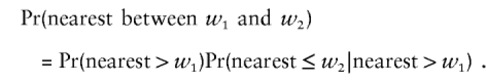
where w is distance measured in Morgans. The probability that the nearest recombination occurred between two marker locations, w₁ nearer and w₂ farther from the disease-susceptibility locus, is Pr(nearest between

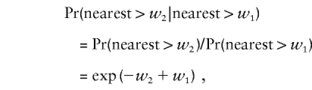
Because of the Poisson property,

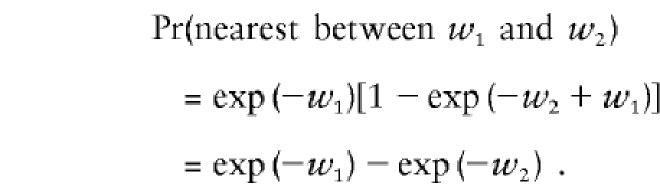
so that

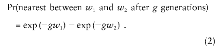
In the next generation, recombination again occurs at random, without regard to previous recombinations. Therefore, the distribution of recombinations occurring in two generations has the same form but double the rate. Linkage interference does not apply in different generations, so that, in multiple generations, its effect rapidly disappears. Thus, for g generations, the rate is simply g times the single-generation rate,

Recombinations occur on both sides of the disease locus. Although restricted by linkage interference in a single generation, recombinations on the two sides are statistically independent in different generations, so, over many generations, the sides are nearly independent. Thus, the joint probability of distances to the nearest recombinant marker on either side of the disease locus is approximately their product.

Confounding Effect of Homozygosity

We do not observe crossovers, only the resulting haplotypes. Because of this, recombination becomes confounded with homozygosity in the parent. To see how, let us calculate trimming probabilities in a single generation for the ancestral allele a, at marker M that is distance w from the disease locus, Dis. In the trimmed-haplotype notation introduced above, preservation of allele a would yield a haplotype included in category D 1, and nonpreservation would fall into category D 0. For haplotype D 1 to have descended from a parent who carried allele a, either no recombination occurred between Dis and M, or a recombination did occur but the parent was homozygous at M. The probability that the parent was homozygous, given that he/she carried allele a, is simply the allele frequency q(a). Thus, Pr(D1)=exp(-w)+[1-exp(-w)]q(a). Without historical information about allele frequencies, we must assume that q(a) has remained approximately the same since the time of the ancestral founder. For haplotype D 0 to have descended from a D 1 parent, a recombination must have occurred in the interval, and the parent must have been heterozygous at M. Thus, Pr(D0)=[1-exp(-w)][1-q(a)]. Note that Pr(D0) and Pr(D1) sum to unity, because they constitute the only possibilities in this situation.

We can calculate trimming probabilities for any number of markers by making a slight change in notation. Consider a haplotype of n markers, M₁–M_n, with ancestral alleles a₁–a_n, whose frequencies are q(a₁)–q(a_n), respectively. Let us write Pr(k,n) for the frequency of a haplotype of n markers with k preserved ancestral markers. For this haplotype to be inherited from a parent carrying the entire ancestral haplotype, two conditions must be met. First, the parent’s marker, M_k+1, must be heterozygous, for a recombination between w_k and w_k+1 to be disclosed. Second, it is possible that there could be a recombination nearer to the disease-susceptibility locus than w_k, but, if so, then all the markers from M_k to the nearest recombination must be homozygous. Thus,

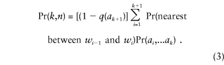To ensure that the first and last terms are correct, we define w₀=0, w_n+1=∞, and . Although markers M_i to M_k, which are confined to a small chromosomal region, may well not be in linkage equilibrium, if the estimation of haplotype frequencies is problematical, we may need to substitute Pr(a_i,...a_k)≈Π^k_j=iq(a_j).

Intervals with Multiple Nearest Recombinations

Equation (3) applies to a single generation, in which multiple recombinations in small intervals are prevented by linkage interference. However, over many generations, the probability that several other recombinations occur in the same marker interval with the nearest recombination to the disease locus may not be negligible. Nonetheless, a simple inductive argument shows that the interaction of heterozygosity, homozygosity, and restoration of the ancestral allele by subsequent recombinations just balances, to retain the same probability of trimming and preservation, regardless of the number of recombinations in the interval.

Let us again consider the case of Dis and only one marker M. Suppose that, after g generations in which there have been m recombinations in the interval w, the alternative probabilities are

and

At the next generation, haplotype D 0 would be inherited from a D 0 parent in absence of recombination. In addition, if a recombination did occur, any parent, D d0 or D 1, would produce a D 0 offspring if the parent carried an allele other than a on the opposite chromosome. Thus,

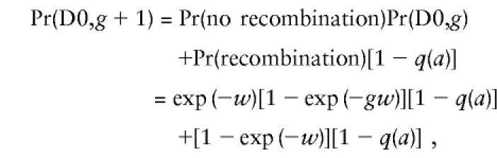so that, reshuffling a bit, . This is the form of equation (4) with gw replaced by (g+1)w. Likewise, D 1 would be produced if a recombination occurred in any parent who happened to carry allele a on the other chromosome.

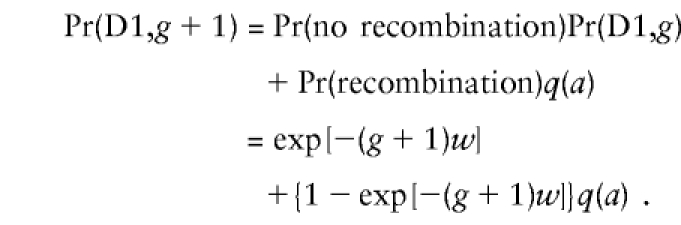This is the form of equation (5) with gw replaced by (g+1)w. Note that the number of recombinations, m, does not appear in these formulas. The argument can easily be extended to chromosomal regions of all sizes, and, in each case, the number of recombinations in the interval containing the nearest recombination is irrelevant.

Thus, formula (3) applies to the case in which multiple nearest recombinations have occurred in the same interval but in different generations.

Historical Changes in Trimmed-Haplotype Frequencies

Over time, a distribution of trimmed haplotypes develops because of the breakup of the ancestral haplotype by recombinations. As generations pass, the distribution shifts toward categories that are less similar to the ancestral founder. Table 2 displays an example of trimmed-haplotype frequencies, calculated as described above, for a haplotype of length 1 cM, measured from marker A to marker F. For the examples in table 2, all interlocus distances are set equal to one-fifth of the total haplotype length, including the distance from the disease locus to its flanking markers. The frequency of each ancestral allele is .2.

Table 2.

Trimmed-Haplotype Table and Category Frequencies

	Haplotypea						No. of Generationsb
Category	A	B	Dis	C	E	F	100	200	300	LEc
1	1	1	D	1	1	1	.389	.173	.075	.000
2	1	1	D	1	1	0	.089	.083	.060	.001
3	0	1	D	1	1	1	.081	.079	.055	.001
4	0	1	D	1	1	0	.018	.038	.044	.005
5	1	1	D	1	0	X	.104	.116	.099	.006
6	X	0	D	1	1	1	.079	.090	.074	.006
7	0	1	D	1	0	X	.021	.053	.073	.026
8	1	1	D	0	X	X	.102	.133	.133	.032
9	X	0	D	1	1	0	.018	.043	.058	.026
10	0	1	D	0	X	X	.021	.061	.097	.128
11	X	0	D	1	0	X	.021	.061	.097	.128
12	X	0	D	0	X	X	.021	.070	.130	.640

^a0, 1, D, and X are as defined for table 1.

^bSince ancestral founder.

^cLE = linkage equilibrium, after many generations.

Among individuals who carry a disease allele descended from an ancestral founder 100 generations in the past, many also carry the entire surrounding ancestral haplotype over a region >1 cM wide (table 2, column 3). At 200 and 300 generations, most haplotypes have been trimmed repeatedly in this region, and, after a sufficiently long time, the distribution of trimmed-haplotype frequencies conforms to the null hypothesis. Although we have shown this as linkage equilibrium for illustrative purposes, in many human populations, markers as tightly linked as those of table 2 are not found in equilibrium, even in the absence of a disease locus. Therefore, the null-hypothesis distribution of trimmed haplotypes in a real test may be quite different from that in column 6 of table 2. It is usually not practical to model category frequencies explicitly for the null hypothesis; rather, we draw a control subsample from observed data.

Because we cannot observe elapsed time since the introduction of the disease allele, the number of generations, g, must be either obtained from other sources or estimated as part of the statistical procedure. We have found that, for large values of g, the ancestral hypothesis becomes indistinguishable from the null hypothesis, and so simultaneous estimation of g within the procedure nullifies the trimmed-haplotype test. Instead, we might use a conjecture based on work of scholars in the history of the relevant population (e.g., Relethford and Crawford ¹⁹⁹⁵; Laan and Pääbo ¹⁹⁹⁷). In the absence of such evidence, an estimate of g can be obtained from marker-to-marker LD in the observed sample. This calculation would use all possible pairs of markers in the chromosomal region and their corresponding distances. Although these pairs would not be statistically independent, this is a small difficulty compared with the assumption that marker age is indicative of the age of the disease locus. Nonetheless, on the basis of a marker-to-marker analysis of the Irish Sample of High-Density Schizophrenia Families, we estimate g to be ∼230±20 generations in the Irish population, leading to preserved regions 1–2 cM in length (Kendler et al. 1998). Fortunately, the parameter g, as long as it is within reasonable bounds, does not play a crucial role in the significance test.

Marker Mutation

The model above applies where breakup of haplotypes occurs solely from recombination. However, with minute chromosomal regions full of microsatellite markers that have unknown and possibly high mutation rates (Weber and Wong 1993), mutation effects need to be represented in the trimmed-haplotype table. Marker mutation has a less drastic effect than does recombination on the haplotype surrounding a disease locus. Recombination at a marker near the disease locus obliterates evidence of a founder throughout the recombinant region, whereas a mutation affects only the marker itself. Therefore, if mutation is also considered, the presence of ancestral alleles at outside markers carries weight, even in the presence of an inside nonidentity.

Recombination replaces alleles in proportion to allele frequencies, but marker mutation produces a different pattern. According to the “stepwise-mutation model” for microsatellite markers (Kimura and Ohta 1978), the characteristic result of a single mutation would be a haplotype with alleles preserved at all markers except the mutated marker, at which the allele would be one repeat longer or one shorter than the former allele. Applying this model, we add a mutation subcategory to each trimmed-haplotype category that arises from recombination. The trimmed-haplotype category positions of haplotypes in mutation subcategories are elevated from the positions they would occupy under a recombination-only model, because we now take into account ancestral alleles in regions that were formerly ignored as recombinant.

Although unequal mutation rates have been demonstrated for different kinds of markers (Chakraborty et al. 1997), it is probably unrealistic to attempt an estimation of separate rates, in most cases. Therefore, let us assume the same mutation rate for all markers in a region and statistically independent mutation events. At a single marker with mutation rate μ per generation, Pr(no mutation in g generations)=(1-μ)^g. An observed haplotype with k markers displaying the ancestral haplotype except for an allele one repeat longer or one shorter than the corresponding ancestral allele, falls into a special trimmed-haplotype category with adjusted trimming probability Pr(k,n,μ)=Pr(k,n)k[1-(1-μ)^g](1-μ)^g(k-1). This category may be shared by haplotypes with apparent mutations at different markers, because the adjustment is independent of location within the trimmed haplotype. To compensate for mutation subcategories, we must adjust the trimming probability for the corresponding category without apparent mutations by a factor of (1-μ)^gk. Mutation is not limited to a single event within the preserved chromosomal region, but haplotypes with multiple mutations would have category frequencies too small to be useful. Therefore, in practice, for the rare cases of multiple apparent mutations, we use only the nearest marker that meets the criteria as a mutation and consider the farther ones to be recombinations. Under the null hypothesis, in which similarity to the ancestral haplotype is fortuitous, the history of recombinations and marker mutations is irrelevant. We simply use the haplotypes that appear in the control sample that meet the particular category criteria.

Inclusion of mutation does not seriously affect a trimmed-haplotype table of only a few markers, but if as many as 10 markers on each side were examined, exclusion of mutation could mean that important similarities would be ignored. Thus, in treating enormous haplotypes (in the analysis of SNPs, for example), mutation becomes more important.

Genotyping Errors

Genotyping errors are resolved as well as possible before trimmed-haplotype analysis, and unresolvable errors are usually coded 0 or blank. Rather than suppressing all haplotypes that contain blank alleles—often several percent of the sample—we treat them somewhat similarly to recombinations. Because we cannot determine whether a missing allele is the ancestral allele, we also cannot know whether the outside markers are relevant to the ancestral hypothesis. We follow the conservative procedure and classify the haplotype as though the missing allele were a crossover. In this case, genotyping errors have the effect of shortening the preserved region of ancestral haplotype and shifting haplotypes to lower positions in the trimmed-haplotype table. In the unknown cases in which the missing allele is actually the ancestral allele, outside ancestral alleles are ignored and some information is lost. However, this method at least allows us to calculate the correct adjustment in category probability, regardless of whether reclassification was really necessary.

Let us call the error rate λ. In the case of a single marker, the trimming probability is increased by the probability that the ancestral allele is actually preserved, but the marker has an error: Pr(D0,λ)=Pr(D0)+Pr(D1)λ. The complimentary probability of preservation is reduced by the same amount: Pr(D1,λ)=Pr(D1)(1-λ).

Extension to the general case, for n markers with k preserved ancestral markers, followed by a blank allele at marker M_k+1, is straightforward. Although treatment could easily be adapted to individual marker error rates if separate estimates exist, the prospect of reliable individual error-rate estimates seems remote. Therefore, let us assume the same independent error rate for all markers. All the k preserved ancestral alleles must avoid error, so that (1-λ)^k is a common factor. In addition, the error at marker M_k+1 reduces the trimmed-haplotype category of any haplotypes that have ancestral alleles between markers M_k+1 and M_n. Thus, Pr(k,n,λ)=(1-λ)^k[Pr(k,n)+λΣⁿ_i=k+1Pr(i,n)].

Uncertain Marker Location

The trimmed-haplotype calculations presented above are based on precise marker locations, whereas in practice we may need to accommodate some uncertainty. Because marker locations generally cannot be determined by linkage analysis more accurately than 1 or even 2 cM (Jorde 1995), for the dense markers required by LD analysis, location must be established by physical mapping. However, physical mapping is still quite expensive, although technology improves continuously. Therefore, at least for now, many problems must be attacked without knowledge of exact marker locations.

In the worst case we may need to fall back on a nonparametric measure of similarity between each category and the ancestral haplotype. For example, we could represent similarity of each trimmed haplotype to the ancestral haplotype by recording the number of ancestral alleles they share, as shown in table 3. This sharing score conforms to our intuitive notion that the haplotypes most similar to the ancestral haplotype are those most likely to have descended from it, but the score requires no specific population-genetic assumptions.

Table 3.

Trimmed-Haplotype Category Similarity Scores

	Haplotypea
Category	A	B	Dis	C	E	Similarity Scoreb
1	1	1	D	1	1	4
2	1	1	D	1	0	3
3	0	1	D	1	1	3
4	0	1	D	1	0	2
5	X	0	D	1	1	2
6	1	1	D	0	X	2
7	X	0	D	1	0	1
8	0	1	D	0	X	1
9	X	0	D	0	X	0

^a0, 1, D, and X are as defined for table 1.

^bMeasured by the number of alleles shared with ancestral haplotype.

Of course, such a score may be a poor representation of the trimming process. The problem can be mitigated if we have partial information that can be used. A semiparametric score might be provided by trimming probabilities calculated with assumed locations, such as the equally spaced lattice distribution used in the example for table 2. If distances between certain markers in the haplotype were known, they could be used as anchors for assumed locations of the remaining markers.

Observed Haplotypes

The observations of the trimmed-haplotype method consist of haplotypes, usually two for each pedigree founder of each pedigree in the sample. Parent-offspring triads have four pedigree-founder haplotypes observed in each family. In complex pedigrees, there may be many more than four pedigree-founder haplotypes. At the other extreme, a pedigree consisting only of a pair of affected sibs, without the parents' being genotyped, may display as few as two haplotypes, if the sibs share both.

The search for disease-susceptibility loci often begins with linkage analysis in chromosomal regions throughout the genome. Because investigators attempt to weed out false positives by intensive genotyping, by the time linkage has been established in a chromosomal region, the sample has usually been genotyped at many markers throughout the region. With this much information, often all pedigree-founder haplotypes in the sample are unique; that is, every pair of haplotypes differs somewhere in the large chromosomal region, although in the minute region of putative LD there may be many duplicates. The entire region, rather than just the putative ancestral subregion, is used to determine the inherited haplotype. Recombinations often occur between the generations observed in sample pedigrees. Outside the ancestral subregion, recombinations do not interfere with the trimmed-haplotype analysis. Even within the small ancestral region, unless the markers flanking the disease-susceptibility locus are affected, the trimmed-haplotype pattern could usually be inferred. However, trimmed-haplotype tests usually use ancestral regions small enough that recombinations within them are rare and can be discarded without serious loss.

An integral part of the trimmed-haplotype method consists in partitioning the sample into test and control subsamples (often called “cases” and controls, but “cases” would be confusing usage in our discussion because many nonancestral cases of affection occur under the null hypothesis). A control subsample is required because we have no theoretical trimmed-haplotype category frequencies under the null hypothesis. Since the markers of such a small region are tightly linked, we cannot rely on the product of allele frequencies to produce haplotype frequencies. An investigator might obtain a control sample from an outside source, but matching has proved problematical in LD analysis, and a control subsample drawn from the same sample as the test subsample is usually preferable (Falk and Rubinstein 1987).

In the TDT, the test subsample consists of transmitted haplotypes, and the control subsample consists of nontransmitted haplotypes, with the two subsamples being of equal size. For multiplex pedigrees, partition of haplotypes into test and control subsamples is somewhat more complicated, but the same principle applies. For example, we might select as controls all haplotypes that appear in pedigrees but that are not transmitted to any affected members. In the Appendix, we describe a method of treating multiplex pedigrees that provides a probabilistic assignment based on a parametric segregation model, which was determined previously. The haplotype-based posterior probability of linkage (HBPPL) can be used as a weight for the corresponding haplotype in the trimmed-haplotype table. Every haplotype is entered in both subsamples: in the test subsample with weight HBPPL and in the control with weight 1-HBPPL. Alternatively, HBPPL can be used as a criterion by which haplotypes with less than a specified value are assigned to the control subsample, and those with a greater value to the test subsample. Under these methods, the test and control subsamples generally do not have the same size.

Let us denote q_i as the observed frequency in category i of the test subsample and p_i as the observed frequency of the controls. Suppose that a certain proportion of haplotypes, α, contain a disease-susceptibility gene in the present chromosomal region, whereas the remainder, 1-α, occur in the absence of linkage. Parameter α accounts for what is called “locus heterogeneity.” The frequency of haplotypes in category i in the absence of linkage is called v_i. Even among those who carry a disease-susceptibility gene, only a proportion δ have inherited it from a particular ancestral founder. Parameter δ accounts for what is called “allelic heterogeneity.” We distinguish “ancestrally derived” haplotypes, with category frequency u_i, from haplotypes that carry a disease allele in the given region but have inherited it from another ancestor, called “causal” haplotypes, with category frequency w_i. Test subsample category frequency q_i derives from all three sources—ancestral, causal, and nonlinkage: q_i=δαu_i+(1-δ)αw_i+(1-α)v_i. Although the distribution of w_i might be somewhat different from that of v_i, causal haplotypes should not be biased with respect to the ancestral haplotype of the present trimmed-haplotype table. Therefore (especially since we have little chance of distinguishing the two, anyway), we assume that causal haplotypes have approximately the null distribution, so that

The Statistical Test

According to the Neyman-Pearson lemma, the most powerful statistic for tests of fully specified hypotheses is the log-likelihood ratio. In our case, in which the observations can be sorted into m trimmed-haplotype category frequencies with a multinomial distribution, the Neyman-Pearson statistic has the form

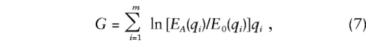where q_i is the observed test subsample frequency of trimmed-haplotype category i, E_A(q_i) is its expected value under the alternative hypothesis, and E₀(q_i) is the expected value under the null hypothesis.

We usually would not have a priori values for E_A(q_i) and E₀(q_i), so they must be estimated, either from the data or from the trimmed-haplotype model. More than one formulation of the likelihood-ratio (LR) test is possible. The most familiar form uses category frequencies estimated from the data themselves. We call this general-purpose LR statistic LR(est). We estimate E_A(q_i) with the category frequency observed in the test subsample, E_A(q_i)=q_i, and the null hypothesis value E₀(q_i)=p_i. Statistic G is not defined when either E_A(q_i)=0 or E₀(q_i)=0, the maximum-likelihood (ML) estimate when the corresponding observed category is empty. To avoid 0, we employ an alternative estimate of E(q_i). We solve for a small constant, ε, that yields Pr(x>0|ε)=Pr(x>1|1/n). That is, we estimate the category frequency that produces the probability of finding >0 where an empty category was observed, equal to the probability of finding >1, given the ML category frequency with one observation. The value is approximately ε=1/3n.

LR(est) does not explicitly use the model on which trimmed-haplotype analysis is based. Therefore, LR(est) responds proportionally to any deviation between the test and control subsamples, positive or negative. To exploit the model of the trimming process, we use it to generate the expected value under the alternative hypothesis in a statistic called LR(trim). We define a category-similarity score, s_i, that measures similarity between haplotypes in category i and their putative ancestor. The trimming probability is the appropriate similarity score when we have enough information to perform the calculations. If the alternative hypothesis is true, including the specific model we use to calculate the trimming probability, then the expected value of u_i equals s_i, and from equation (6), E_A(q_i)=δαs_i+(1-δα)E_A(v_i). Since our most uncontaminated information about the null hypothesis population comes from the control subsample, E_A(v_i) is estimated by p_i. Therefore, under the alternative hypothesis the expected value is estimated by E_A(q_i)=δαs_i+(1-δα)p_i, whereas, under the null hypothesis, the expected value is estimated simply by E₀(q_i)=p_i.

If the model of disequilibrium we employ in LR(trim) is correct, or nearly correct, LR(trim) should have a considerable advantage over LR(est). However, LR(trim) depends on several parameters that we may not be able to estimate accurately—locus and allelic heterogeneity, as well as the number of generations elapsed since the founding ancestor and the marker mutation rate. Under poor assumptions, the parametric approach may perform worse than LR(est). Either formulation is valid; the issue depends entirely on statistical power.

Bootstrap Significance Level

Because sampling distributions of the trimmed-haplotype test may be quite complicated, we calculate significance levels for the trimmed-haplotype statistic, using random-permutation replications (Efron and Tibshirani 1993). The method falls under the general heading of bootstrap techniques, a class of methods to assess statistical significance that avoid our having to make assumptions regarding the asymptotic behavior of statistics (Efron 1982). To avoid being misled by the presence of linkage alone, we wish to conditionthe distribution on whatever linkage signal is present in the data. Therefore, replicates are formed by the shuffling of haplotype designations among pedigrees while patterns of inheritance are kept intact. The assignment of pedigree-founder haplotypes to the test and control subsamples remains constant, but their assignment to trimmed-haplotype categories varies. The simulated statistic,

calculated over many replications, provides a distribution against which the observed statistic, G, can be measured. Large values of G occur when high observed-category frequencies in the test sample coincide with a predicted excess of trimmed haplotypes over controls. In replicate samples under the null hypothesis, q_ih has the same distribution, on average, as p_i, and any excess is random. Therefore, the “achieved significance level” of a test is the rank order of G for the actual observed sample, relative to the population of simulated samples R_h.

Let us illustrate the construction of achieved significance levels with a simplified example. Consider two diallelic markers with the disease locus between them. The sequence of marker haplotypes that are assigned putative ancestral status runs through all four possible haplotypes. For each analysis, we calculate the observed statistic G and 10 replicates, R₁–R₁₀, as shown in table 4. We calculate the haplotype-specific significance level for each putative ancestral haplotype by counting the number of replications R_h that exceed G. In our example, haplotype 1 1 has the achieved significance level .6, haplotype 1 2 has significance level .1, haplotype 2 1 has significance level .8, and haplotype 2 2 has significance level .3.

Table 4.

Bootstrap Calculations for Haplotypewise Significance Level

	Replication Score for Ancestral Haplotypea
Sample	1 1	1 2	2 1	2 2
Observed (G)	1.4	4.8	.8	2.6
Replicate:
R1	.2	2.4	1.1	.7
R2	1.9	4.1	.7	1.4
R3	1.1	.9	1.7	4.6
R4	3.7	2.8	2.1	3.4
R5	1.4	2.4	2.5	2.1
R6	2.8	3.7	1.7	2.4
R7	3.5	5.0	4.2	2.1
R8	.7	2.9	.6	4.9
R9	2.1	2.0	1.0	1.9
R10	1.3	2.7	1.1	2.5

^aScores exceeding the observed score are underlined.

Repeated Analysis and Significance Level

The trimmed-haplotype method uses only one ancestral haplotype in each trimmed-haplotype table. Except in an attempt to replicate a specific finding from other data, we would rarely have a particular ancestral haplotype hypothesized beforehand. Several current LD methods (Sham and Curtis 1995; Terwilliger ¹⁹⁹⁵) treat the entire set of alleles at a given marker locus simultaneously and produce an overall significance level (extension to simultaneous treatment of multiple-marker haplotype data is straightforward). The drawback to simultaneous testing is that a true excess in one or a few haplotypes may be confounded with many small differences, randomly distributed between excess and dearth. In high-density samples, haplotypes with too few transmissions are probably not causally related to a disease-susceptibility gene. The problem is especially acute among the huge number of possible haplotypes of a region with multiple, highly polymorphic markers. The trimmed-haplotype method of treating all haplotypes of a given set of markers consists in repeated testing of admissible combinations of alleles at the markers. We may exclude alleles with extremely low observed frequencies from the admissible set, since they could not contribute very much to high trimmed-haplotype scores anyway.

Alleles are not the only familiar uncertainty. In most cases, the location of the disease locus cannot be specified precisely beforehand. Such uncertainties apply to any method of LD analysis, and the usual solution is to test all admissible locations in the chromosomal region, producing a map analogous to a multipoint linkage map. A new trimmed-haplotype table must be constructed for each marker interval in which the disease locus is hypothesized, and every location throughout the chromosomal region generates a separate set of trimming probabilities. We might also need to try haplotypes of different sizes, from only two flanking markers to larger chromosomal regions, searching for the most positive results among all these tests. Marker order is especially important to the trimmed-haplotype analysis, because assignment to trimmed-haplotype categories depends on the nearest recombination on both sides of a putative disease locus. If the order of all markers is not known with certainty, as often happens, we must also repeat the analysis using marker combinations compatible with the subset of markers of known order.

Of course, type 1 errors would be inflated by this repeated analysis and must be taken into account. Each putative ancestral haplotype that is analyzed has a corresponding significance level. However, the sequence of ancestral haplotypes analyzed for a given combination of markers is highly correlated, since alleles are cycled on and off the putative ancestral haplotype one at a time. Thus, it would be highly inaccurate to use any sort of Bonferroni correction to adjust for multiple testing. Instead, we use an extension of the bootstrap method by recording the best haplotype for each randomized replication. Then the best-observed haplotype of the actual sample is sorted in among the best replicate-sample scores. Its rank order in this select set is the global significance level of the best putative ancestral haplotype over all haplotypes for a particular combination of markers. To extend our example from table 4 above, we use the same data to calculate row maxima, as shown in table 5. Then we count the number of replications in which the row maximum exceeds the maximum for the observed data. In our example there are two such replications, so the global significance level is .2.

Table 5.

Bootstrap Calculations for Global Significance Level

	Ancestral Haplotypea
Sample	1 1	1 2	2 1	2 2
Observed (G)	1.4	4.8	.8	2.6
Replicate:
R1	.2	2.4	1.1	.7
R2	1.9	4.1	.7	1.4
R3	1.1	.9	1.7	4.6
R4	3.7	2.8	2.1	3.4
R5	1.4	2.4	2.5	2.1
R6	2.8	3.7	1.7	2.4
R7	3.5	5.0	4.2	2.1
R8	.7	2.9	.6	4.9
R9	2.1	2.0	1.0	1.9
R10	1.3	2.7	1.1	2.5

^aThe best haplotype score for each replication is underlined, and those exceeding the best observed score are also shown in boldface type.

Under the null hypothesis, the distribution of trimmed-haplotype scores depends somewhat on the frequencies of the putative haplotype and those closely related to it. Therefore, to compare separate putative haplotypes, the values must be standardized. The ideal way to achieve this would be to transform the procedure into the P-value domain, which generates a uniform scale (Efron and Tibshirani 1993). However, for this method, each replicate would require its own set of replicates to produce its significance level. This would square the computational effort required and would probably be infeasible. A more economical alternative is to standardize the trimmed-haplotype scores themselves. Although, in general, the distribution of trimmed-haplotype scores is skewed, we have found in simulations that adjustment by mean and variance produces distributions with no bias in favor of any particular haplotype under the null hypothesis. That is, the best trimmed-haplotype score is distributed randomly among all haplotypes, in their role as putative ancestral haplotype, without regard to haplotype frequencies.

Effect of Heterogeneity

The trimmed-haplotype method is designed especially for the case in which haplotypes that bear the disease gene account for a small fraction of all observed haplotypes. Heterogeneity is not treated explicitly in LR(est), but it does appear in LR(trim). We usually would not have an accurate estimate of the heterogeneity parameters α and δ, describing locus and allelic heterogeneity, respectively. However, it turns out that, as long as their product is small, precise estimates of δ and α are not essential. To see why, recall from the Taylor series that ln(1+x)≈x in a tight neighborhood of x=0. The LR(trim) statistic can be written

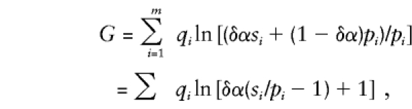so that, when δα is small, . Since δα is common to all categories, and the same is true in all replications, , parameter δα would cancel out of the achieved significance-level calculation. Although we do not actually make the substitution, this approximation shows that no small value of δα could affect the trimmed-haplotype test very much.

In a complex disease, δα must often be small. Many haplotypes belong to unaffected individuals; others come from sporadic cases or from affection caused by loci in other regions. Small values of α could be expected in a disease such as schizophrenia, in which linkage has been reported and replicated in 11 chromosomal regions (Crow and DeLisi ¹⁹⁹⁸). If most of these regions actually are linked, the average α value must be small.

In some cases, we might have a degree of evidence about α from the admixture model of linkage analysis (Smith 1963), but there is usually no evidence about δ except from trimmed-haplotype analysis itself. The trimmed-haplotype test need not be confined to a single putative haplotype. If different ancestral haplotypes surrounded the disease-susceptibility gene in separate founders, each may give rise to moderately elevated trimmed-haplotype scores. We can use the same set of replication scores to assess the significance level of not only the best observed haplotype but also the second-best and subsequent scores. For example, a test for the second-best haplotype of the marker combination can be demonstrated on the data of tables 4 and 5, although, in a real study, we would not search for more ancestral haplotypes if the most outstanding one had significance level of only .2. However, for illustrative purposes, consider table 6. Haplotype 2 2 has the second-highest value of G at the marker combination. Among the second-highest scores of all replications, four exceed the second-highest value of G, so that the achieved significance level of a second ancestral haplotype is .4. In a real study, we would search for a break-point at which the first n observed P values are more extreme than their corresponding replicates and subsequent observed values fall into the middle of the corresponding replicate distributions. Examination of the alleles common to these n best-scoring haplotypes might indicate something of the relevant history. Haplotype clusters that share alleles around the disease-susceptibility locus may descend from early recombinations in the same ancestral haplotype. On the other hand, haplotypes that differ even in the nearest flanking markers probably descend from different ancestral founders.

Table 6.

Bootstrap Significance Level for Second-Best Haplotype

	Ancestral Haplotypea
Sample	1 1	1 2	2 1	2 2
Observed (G)	1.4	4.8	.8	2.6
Replicate:
R1	.2	2.4	1.1	0.7
R2	1.9	4.1	.7	1.4
R3	1.1	.9	1.7	4.6
R4	3.7	2.8	2.1	3.4
R5	1.4	2.4	2.5	2.1
R6	2.8	3.7	1.7	2.4
R7	3.5	5.0	4.2	2.1
R8	.7	2.9	.6	4.9
R9	2.1	2.0	1.0	1.9
R10	1.3	2.7	1.1	2.5

^aThe second-best haplotype score for each replication is underlined, and those exceeding the second-best observed score are also shown in boldface type.

The worst possibility for heterogeneity is that a large number of separate disease mutations might have arisen over time, so that even in a large sample, a given mutation would manifest itself in only one or two pedigrees. Although this has proved not to be the case for relatively simple diseases, such as cystic fibrosis (Ramsay et al. 1993), congenital chloride diarrhea (Höglund et al. 1995), and Werner syndrome (Goddard et al. 1996), there is no guarantee that it is not true of common, complex disorders. There are known instances of loci at which multiple independent mutations have arisen; for example, β-hemoglobin (Vogel and Motulsky 1997, p. 313). This presents a hopeless situation to the trimmed-haplotype method, since the haplotypes would be distributed approximately according to null-hypothesis category frequencies, even though many may have arrived by an ancestral route. Although evidence for linkage may well be strong, any type of LD analysis would probably fail in this case.

Operational Characteristics

We have performed a series of simulation experiments to benchmark the performance of the trimmed-haplotype method. Full results are presented in a companion paper (R.B. Martin, C.J. McLean, R.E. Straub, and K.S. Kendler, in preparation). In brief, results show that the trimmed-haplotype method produces the proper type 1 error rate under the null hypothesis and is not misled by the presence of intense linkage or even LD, as long as it is not correlated with the putative ancestral haplotype. We have also performed a series of statistical power simulations under a variety of alternative hypotheses, including locus and allelic heterogeneity, various sizes of ancestral haplotypes, and various pedigree structures. For comparison, we included two commonly used LD methods, ETDT (Sham and Curtis 1995) and DISMULT (Terwilliger 1995). In general, the trimmed-haplotype method performed well.

Software

The trimmed-haplotype test has been implemented in a computer package written by R. B. Martin. The program, called TRIMHAP, is freely available to all investigators from the TRIMHAP World Wide Web site.

We have designed the package to operate along the same lines as LINKAGE, offering a choice of options such as parametric or nonparametric analyses, with the whole process controlled from a shell-like interface. We assume that the user supplies a grid of markers covering some chromosomal region and has constructed haplotypes using software such as GENEHUNTER. In the first step of TRIMHAP, the user is asked to define a subset of markers that are feasible as ancestral haplotypes, and only markers in this subset are scanned. The user then defines the number of markers in the putative ancestral haplotype and may choose to fix some or all of them. If an ancestral marker locus is fixed, the corresponding allele may be fixed or left free, so that all alleles are tested. The location of the disease locus within the ancestral haplotype can also be specified or left to vary.

TRIMHAP next examines all combinations of markers and alleles compatible with the above restrictions, to construct a sequence of ancestral haplotypes to analyze. If map order is known, only contiguous markers are scanned; if partially unknown, all admissible combinations, subject to user specifications, are examined. Two filters are used to reduce combinations. The user can specify a maximum span in centimorgans for the putative ancestral haplotype and can also set a minimum allele frequency for ancestral alleles.

Once an ancestral haplotype is chosen, TRIMHAP determines identity by descent within the pedigree. For each haplotype in the sample, a haplotype-sharing score is calculated. Either the trimming probability or the number of alleles in common with the putative ancestral haplotype are calculated, at the user’s option. TRIMHAP determines the category of each haplotype, adds it to the trimmed-haplotype table, and constructs the sum of haplotype-sharing scores over all categories. Empirical P values are calculated by use of a rapid haplotype-permutation scheme. The chromosomal region is scanned over the sequence of putative ancestral haplotypes specified, and the whole process is replicated to construct global empirical P values.

Appendix: Haplotype Analysis in Multiplex Pedigrees

Parametric treatment of pedigrees requires an assumed segregation model. Although segregation models of complex diseases are rarely known, linkage analysis often offers support for one mode of inheritance over others. Genetic software such as GENEHUNTER provides ML marker haplotypes for all pedigree members, and a simple algorithm determines which parental haplotype is inherited in each transmission throughout the pedigree. We construct a probability for each possible disease-gene configuration in a pedigree and then sum up, for each pedigree-founder haplotype in turn, the probabilities of all disease configurations in which the haplotype contains the disease-susceptibility allele. This yields an HBPPL that can be used as a weight for the corresponding haplotype in the trimmed-haplotype table.

It might be helpful to consider a specific example, shown in figure 1. Pedigree members A and B are parents of the sibship C, E, and F, of whom two are affected. Since only the two parents are founders of this pedigree, there are four haplotypes to consider. Although these may be multiple-marker haplotypes, let us label them simply 1, 2, 3, and 4, disallowing recombination within a haplotype among the transmissions of this family. Intuitively, haplotype 1 in figure 1 gives the strongest contribution to affection since it is passed to both affected offspring. Haplotype 4 would probably be ranked next, since it is passed to an affected offspring only, whereas haplotype 3 is passed to one affected and one unaffected offspring. Haplotype 2 is passed only to an unaffected offspring and would be ranked last. Let us quantify these notions in table A1.

Figure 1.

Sample pedigree used in table A1

Table A1.

Probabilities of All Potential Disease-Allele Configurations

	Parents				Offspring						Probabilities
Configuration	1	2	3	4	1	3	1	4	2	3	Priora	Likelihoodb	Jointc
1	d	d	d	d	d	d	d	d	d	d	.960 596	.000 376	.267
2	D	d	d	d	D	d	D	d	d	d	.009 703	.092 198	.662
3	d	D	d	d	d	d	d	d	D	d	.009 703	.000 141	.001
4	d	d	D	d	d	D	d	d	d	D	.009 703	.002 822	.021
5	d	d	d	D	d	d	d	D	d	d	.009 703	.004 610	.033
6	D	D	d	d	D	d	D	d	D	d	.000 098	.018 816	.002
7	D	d	D	d	D	D	D	d	d	D	.000 098	.069 120	.005
8	D	d	d	D	D	d	D	D	d	d	.000 098	.112 896	.008
9	d	D	D	d	d	D	d	d	D	D	.000 098	.000 576	.000
10	d	D	d	D	d	d	d	D	D	d	.000 098	.001 728	.000
11	d	d	D	D	d	D	d	D	d	D	.000 098	.018 816	.002
12	D	D	D	d	D	D	D	d	D	D	.000 001	.007 680	.000
13	D	D	d	D	D	d	D	D	D	d	.000 001	.023 040	.000
14	D	d	D	D	D	D	D	D	d	D	.000 001	.046 080	.000
15	d	D	D	D	d	D	d	D	D	D	.000 001	.003 840	.000
16	D	D	D	D	D	D	D	D	D	D	.000 000	.005 120	.000

^aHigh-risk allele frequency, q=.01.

^bPenetrances, f(DD)=.80, f(dD)=.40, f(dd)=.02.

^cNormed.

To include all configurations of disease alleles D and d in a pedigree with n founders, we need to consider 2²ⁿ possible vectors, each of length 2n. If we assume independence, the prior probability of a vector with m alleles of type D and 2n-m alleles of type d is q^m(1-q)^2n-m, where q is the frequency of D. For our example, let us assume that q=.01, so that in table A1 the prior probability of each vector is .01^m .99^4−m.

Given the distribution of disease alleles among its haplotypes, the pedigree likelihood depends on the transmission of haplotypes throughout the pedigree, together with the affection status of each pedigree member. Although carriers of the disease mutation cannot be observed, they have a probability of affection defined by the penetrance of their genotypes, from the segregation model: f(DD) for affected carriers of genotype DD, 1-f(dD) for normal carriers of dD, etc. Let us assume penetrances of f(DD)=.80, f(dD)=.40, and f(dd)=.02. Since, under our segregation model, affection status is independently assorted, the likelihood of a hypothetical vector of disease alleles is the product of these penetrances, one for each pedigree member. For example, the first vector, d d d d, has likelihood .98×.98×.02×.02×.98≈.0004, whereas the second, D d d d, has likelihood .60×.98×.40×.40×.98≈.09. The product of the prior probability and likelihood produces the joint probability of each possible configuration, and, since the list of 16 haplotype-configuration vectors is exhaustive, these joint probabilities may be normed over the table, to produce posterior probabilities.

Finally, to evaluate the HBPPL for each parental haplotype, we sum the probabilities of vectors in which the haplotype contains D. For each haplotype, this constitutes one-half of the vectors, and there is considerable overlap. HBPPLs do not sum to unity for a pedigree, because of the overlap and because the sporadic disease configuration d d d d does not contribute to any haplotype. Note that the HBPPL values in table A2 correspond well to our intuitive estimates from figure 1, with haplotype 1 by far the most likely contributor, haplotype 2 quite implausible, and haplotypes 3 and 4 about equally unlikely.

Table A2.

Summation for HBPPL from Configuration Probabilities in Table A1

	Disease Allele					HBPPL
Configuration	1	2	3	4	Joint Probability	1	2	3	4
1	d	d	d	d	.267
2	D	d	d	d	.662	.662
3	d	D	d	d	.001		.000
4	d	d	D	d	.021			.020
5	d	d	d	D	.033				.033
6	D	D	d	d	.002	.000	.000
7	D	d	D	d	.005	.010		.000
8	D	d	d	D	.008	.000			.010
9	d	D	D	d	.000		.000	.000
10	d	D	d	D	.000		.000		.000
11	d	d	D	D	.002			.000	.000
12	D	D	D	d	.000	.000	.000	.000
13	D	D	d	D	.000	.000	.000		.000
14	D	d	D	D	.000	.000		.000	.000
15	d	D	D	D	.000		.000	.000	.000
16	D	D	D	D	.000	.000	.000	.000	.000
Total					1.0	.677	.000	.030	.043

References

- Boehnke M (1994) Limits of resolution of genetic linkage studies: implications for the positional cloning of human disease genes. Am J Hum Genet 55:379–390 [PMC free article] [PubMed]
- Chakraborty R, Kimmel M, Stivers DN, Davison LJ, Deka R (1997) Relative mutation rates at di-, tri-, and tetranucieotide microsatellite loci. Proc Natl Acad Sci USA 94:1041–1046 [DOI] [PMC free article] [PubMed]
- Clayton D, Jones H (1999) Transmission/disequilibrium tests for extended marker haplotypes. Am J Hum Genet 65:1161–1169 [DOI] [PMC free article] [PubMed]
- Crow TJ, DeLisi LE (1998) The chromosome workshops at the 5th International Congress of Psychiatric Genetics—the weight of the evidence from genome scans. Psychiatr Genet 8:59–61 [DOI] [PubMed]
- Devlin B, Risch N (1995) A comparison of linkage disequilibrium measures for fine-scale mapping. Genomics 29:311–322 [DOI] [PubMed]
- Efron B (1982) The Jackknife, the bootstrap and other resampling plans. SIAM, Philadelphia [Google Scholar]
- Efron B, Tibshirani RJ (1993) An introduction to the bootstrap. Chapman & Hall, New York [Google Scholar]
- Falk CT, Rubinstein P (1987) Haplotype relative risks: an easy reliable way to construct a proper control sample for risk calculations. Ann Hum Genet 51:227–233 [DOI] [PubMed]
- Goddard KAB, Yu C, Oshima J, Miki T, Nakura J, Piussan C, Martin GM, et al (1996) Toward localization of the Werner syndrome gene by linkage disequilibrium and ancestral haplotyping: lessons learned from analysis of 35 chromosome 8pll.1-21.1 markers. Am J Hum Genet 58:1286–1302 [PMC free article] [PubMed]
- Höglund P, Sistonen P, Norio R, Holmberg C, Dimberg A, Gustavson K, de la Chapelle A, et al (1995) Fine mapping of the congenital chloride diarrhoea gene by linkage disequilibrium. Am J Hum Genet 57:95–102 [PMC free article] [PubMed]
- Jorde LB (1995) Linkage disequilibrium as a gene-mapping tool. Am J Hum Genet 56:11–14 [PMC free article] [PubMed]
- Kendler KS, MacLean CJ, Ma Y, O'Neill FA, Walsh D, Straub RE (199p) Marker to marker linkage disequilibrium on chromosomes 5q, 6p and 8p in Irish high density schizoprenia pedigrees. Am J Med Genet 88(1):29–33 [DOI] [PubMed]
- Kimura M, Ohta T (1978) Stepwise mutation model and distribution of allelic frequencies in a finite population. Proc Natl Acad Sci USA 75:2868–2872 [DOI] [PMC free article] [PubMed]
- Laan M, Pääbo S (1997) Demographic history and linkage disequilibrium in human populations. Nat Genet 17:435–438 [DOI] [PubMed]
- Lazzeroni LC (1998) Linkage disequilibrium and gene mapping: an empirical least-squares approach. Am J Hum Genet 62:159–170 [DOI] [PMC free article] [PubMed]
- McPeek MS, Strahs A (1999) Assessment of linkage disequilibrium by the decay of haplotype sharing, with application to fine-scale genetic mapping. Am J Hum Genet 65:858–875 [DOI] [PMC free article] [PubMed]
- Ott J (1991) Analysis of human genetic linkage. 2d ed. Johns Hopkins, Baltimore [Google Scholar]
- Ramsay M, Williamson R, Estivill X, Wainwright BJ, Ho MF, Halford S, Kere J, et al (1993) Haplotype analysis to determine the position of a mutation among closely linked DNA markets. Hum Mol Genet 2:1007–1014 [DOI] [PubMed]
- Relethford JH, Crawford ME (1995) Anthropometric variation and the population history and genetic structure in Ireland. Am J Phys Anthropol 96:25–38 [DOI] [PubMed]
- Sham PC, Curtis D (1995) An extended transmission/disequilibrium test (TDT) for multi-allele marker loci. Ann Hum Genet 59:323–336 [DOI] [PubMed]
- Smith CAB (1963) Testing for heterogeneity of recombination fraction values in human genetics. Ann Hum Genet 27:175–182 [DOI] [PubMed] [Google Scholar]
- Spielman RS, McGinnis RE, Evens WJ (1993) Transmission test for linkage disequilibrium: the insulin gene region and insulin-dependent diabetes mellitus (IDDM). Am J Hum Genet 52:306–516 [PMC free article] [PubMed] [Google Scholar]
- Stine OC, Xu J, Koskela A, McMahon FJ, Gschwend M, Friddle C, Clark CD, et al (1995) Evidence for linkage of bipolar disorder to chromosome 18 with a parent-of-origin effect. Am J Hum Genet 57:1385–1394 [PMC free article] [PubMed]
- Straub RE, MacLean CJ, O’Neill FA, Burke J, Murphy B, Duke F, Webb BT, et al (1995) A potential vulnerability locus for schizophrenia on chromosome 6p24-22: evidence for genetic heterogeneity. Nat Genet 11:287–293 [DOI] [PubMed]
- Terwilliger JD (1995) A powerful likelihood method for the analysis of linkage disequilibrium between trait loci and one or more polymorphic marker loci. Am J Hum Genet 56:777–787 [PMC free article] [PubMed]
- Vogel V, Motulsky AG (1997) Human genetics: problems and approaches. Springer, Berlin [Google Scholar]
- Weber JL, Wong C (1993) Mutation of human short tandem repeats. Hum Mol Genet 2:1123–1128 [DOI] [PubMed]
- Xiong NI, Guo S (1997) Fine-scale genetic mapping based on linkage disequilibrium: theory and applications. Am J Hum Genet 60:1513–1531 [DOI] [PMC free article] [PubMed]
- Zouali H, Hani EH, Philippi A, Vionnet N, Beckmann JS, Demenais F, Froguel P (1997) A susceptibility locus for early-onset non-insulin dependent (type 2) diabetes mellitus maps to chromosome 20q, proximal to the phosphoenolpyruvate carboxykinase gene. Hum Mol Genet 6:1401–1408 [DOI] [PubMed]