A Model for Shear Stress Sensing and Transmission in Vascular Endothelial Cells

Abstract

Arterial endothelial cell (EC) responsiveness to flow is essential for normal vascular function and plays a role in the development of atherosclerosis. EC flow responses may involve sensing of the mechanical stimulus at the cell surface with subsequent transmission via cytoskeleton to intracellular transduction sites. We had previously modeled flow-induced deformation of EC-surface flow sensors represented as viscoelastic materials with standard linear solid behavior (Kelvin bodies). In the present article, we extend the analysis to arbitrary networks of viscoelastic structures connected in series and/or parallel. Application of the model to a system of two Kelvin bodies in parallel reveals that flow induces an instantaneous deformation followed by creeping to the asymptotic response. The force divides equally between the two bodies when they have identical viscoelastic properties. When one body is stiffer than the other, a larger fraction of the applied force is directed to the stiffer body. We have also probed the impact of steady and oscillatory flow on simple sensor-cytoskeleton-nucleus networks. The results demonstrated that, consistent with the experimentally observed temporal chronology of EC flow responses, the flow sensor attains its peak deformation faster than intracellular structures and the nucleus deforms more rapidly than cytoskeletal elements. The results have also revealed that a 1-Hz oscillatory flow induces significantly smaller deformations than steady flow. These results may provide insight into the mechanisms behind the experimental observations that a number of EC responses induced by steady flow are not induced by oscillatory flow.

INTRODUCTION

By virtue of their location at the interface between the bloodstream and the vascular wall, arterial endothelial cells (ECs) are continuously exposed to a highly dynamic shear (or frictional) stress environment. The ability of ECs to respond and adapt to changes in fluid mechanical shear stress is essential for fundamental processes including vasoregulation in response to acute changes in blood flow and arterial wall remodeling in response to chronic hemodynamic alterations (Pohl et al., 1986; Langille and O'Donnell, 1986). Furthermore, abnormalities and/or inadequacies in endothelial responsiveness to shear stress are involved in the development of atherosclerosis (Nerem, 1992; Davies, 1995).

Recent research has established that shear stress intricately regulates EC structure and function. This occurs via a coordinated sequence of biological events that begins with very rapid responses that include activation of flow-sensitive K⁺ and Cl⁻ channels (Olesen et al., 1988; Jacobs et al., 1995; Barakat et al., 1999; Nakao et al., 1999) and of GTP-binding proteins (G-proteins) (Gudi et al., 1996, 1998), changes in cell membrane fluidity (Haidekker et al., 2000; Butler et al., 2001) and intracellular pH (Ziegelstein et al., 1992), and mobilization of intracellular calcium (Dull and Davies, 1991; Ando et al., 1988; Shen et al., 1992; Geiger et al., 1992). These rapid responses are followed by stimulation of mitogen-activated protein kinase signaling (Traub and Berk, 1998), activation of a host of gene and protein regulatory responses (Malek and Izumo, 1994; Resnick and Gimbrone, 1995; Garcia-Cardena et al., 2001), and induction of extensive cytoskeletal remodeling that ultimately leads to cellular elongation in the direction of the applied shear stress (Dewey et al., 1981; Nerem et al., 1981; Eskin et al., 1984).

Beyond being merely responsive to shear stress, ECs respond differently to different types of shear stress. For instance, while steady shear stress induces intracellular calcium oscillations and morphological changes in ECs, purely oscillatory flow (zero net flow rate) does not elicit either of these responses (Helmlinger et al., 1991, 1995). A number of shear stress-responsive genes also exhibit differential responsiveness to different types of shear stress (Chappell et al., 1998; Lum et al., 2000; Garcia-Cardena et al., 2001). The notion of differential responsiveness is especially significant in light of the observation that early atherosclerotic lesions localize preferentially in arterial regions exposed to low and/or oscillatory shear stress while regions subjected to high and unidirectional shear stress remain largely spared (Nerem, 1992; Ku et al., 1985; Asakura and Karino, 1990).

The mechanisms by which ECs respond to shear stress and by which they discriminate among different types of shear stress remain to be elucidated. A working model for EC flow responsiveness has been proposed and is schematically depicted in our Fig. 1 (see also Davies and Tripathi, 1993; Davies, 1995). This model, which is inspired by the tensegrity hypothesis of cellular mechano-responsiveness (Ingber, 1993; Ingber et al., 1994), postulates that the fluid mechanical stimulus is sensed by structures at the EC surface that act as flow sensors. Flow sensors may be discrete transmembrane molecules, clusters of such molecules, subdomains of the cell membrane, or even the entire membrane. Once sensed, the flow signal is transmitted via cytoskeleton to various intracellular sites including the nucleus, cell-cell adhesion proteins, and focal adhesion sites where it is transduced to a biochemical response. This proposed mechanotransduction scheme should be viewed as complementary to the more well characterized receptor-mediated signaling pathways that exist in vascular ECs.

FIGURE 1.

Schematic diagram of the working model for endothelial shear stress sensing and transmission. Cell-surface flow sensors (which may be discrete structures, cell membrane microdomains, or the entire cell membrane) detect a flow stimulus and transmit it directly via cytoskeleton to various intracellular transduction sites including the nucleus, cell-cell adhesion proteins, and focal adhesion sites on the abluminal cell surface.

We recently developed a model of the deformation of an EC-surface flow sensor in response to different types of shear stress (Barakat, 2001). The flow sensor was modeled as a viscoelastic material with standard linear solid behavior. The results demonstrated that the peak sensor deformation was considerably larger for steady and nonreversing pulsatile flow than for purely oscillatory flow. It was hypothesized that this may constitute a mechanism by which ECs differentially respond to different types of flow. Because the mechanotransduction model shown in Fig. 1 postulates that flow sensors on the EC surface are directly coupled to cytoskeletal elements that are in turn coupled to various intracellular structures, it is essential to extend the results of our previous model to include these couplings. The present article extends the one-body analysis to networks of viscoelastic bodies that represent coupled systems of cell-surface sensors and various intracellular structures. The deformations of the various network components in response to different types of flow and the sensitivities of these deformations to various model parameters are presented.

MATHEMATICAL DEVELOPMENT

Formulation of governing equations

Our goal is to develop a mathematical framework to describe the deformations of EC-surface flow sensors and coupled intracellular structures in response to either steady or purely oscillatory flow. Similar to our previous analysis (Barakat, 2001), each structure is modeled as a viscoelastic body with standard linear solid behavior (Kelvin body) and characterized by its own set of viscoelastic parameters. As described elsewhere (Fung, 1981; Barakat, 2001), a Kelvin body consists of a linear spring with spring constant k₁ (spring 1) in parallel with a Maxwell body, which consists of a linear spring with spring constant k₂ (spring 2) in series with a dashpot with coefficient of viscosity μ. Kelvin bodies are general linear viscoelastic models, and they have been frequently used to represent the mechanical behavior of various tissues. Of specific interest to the present formulation, recent experimental studies have expressed the viscoelastic properties of cell nuclei (Guilak et al., 2000), cytoskeletal elements (Sato et al., 1996), and transmembrane proteins (Bausch et al., 1998), in terms of the parameters of a Kelvin body.

We begin by deriving the formulation describing the deformations of n-Kelvin bodies connected either in series or in parallel and discuss solutions to the governing equations under both steady and oscillatory forcing functions. We subsequently describe simple networks that consist of combinations of Kelvin bodies connected in series and parallel and that are used to model mechanical signal transmission in ECs. Finally, we discuss the implications of the results to overall EC responsiveness to different types of shear stress.

Kelvin bodies in series

Fig. 2 A depicts a system of n-Kelvin bodies connected in series. For a forcing function F(t) applied to this series of n-bodies, the force experienced by each body in the series will be F(t); thus,

(1)

FIGURE 2.

Schematic diagram of n-Kelvin bodies coupled (A) in series and (B) in parallel. Each body consists of a linear spring with spring constant k₁ in parallel with a Maxwell body, which consists of a linear spring with spring constant k₂ in series with a dashpot with coefficient of viscosity μ.

The deformation of the entire series is given simply as the sum of the individual deformations:

(2)

As shown elsewhere (Fung, 1981; Barakat, 2001), the deformation u_i(t) of the i^th Kelvin body given a forcing function F(t) across this body is governed by the following first-order linear differential equation:

(3)

where and are the time derivatives of F and u_i, respectively. We consider that the force F(t) due to fluid flow is applied suddenly at t = 0 as a step function and that this force is sustained for the entire time period considered. Because we wish to investigate the effects of both steady and oscillatory flow, two types of forcing functions are considered. For steady flow, the forcing function takes the form:

(4)

whereas for oscillatory flow, the equivalent expression is:

(5)

where ω is the angular frequency of oscillation. For both types of forcing functions, the applied force at t = 0 is F(0) = F₀. For a suddenly applied force F₀, the appropriate initial condition for the i^th body in the series is (Barakat, 2001):

(6)

For a given forcing function (either Eq. 4 or 5), Eq. 3 can be solved subject to the initial condition in Eq. 6 to yield the deformation u_i(t) for each body in the series. The deformations of the individual bodies are independent of one another and can therefore be solved for separately. Analytic solutions to the deformation of a single Kelvin body for both steady and oscillatory flow are given elsewhere (Barakat, 2001). For the sake of consistency with the formulation of the Kelvin bodies connected in parallel, we have opted to write down the problem in matrix notation as:

(7)

with the initial condition

(8)

where we define

Kelvin bodies in parallel

We can now develop the formulation for n-Kelvin bodies coupled in parallel (Fig. 2 B). There are two fundamental differences between the parallel and series formulations. First, in the parallel case all n-bodies are constrained to deform equally so that

(9)

Secondly, the total force acting on the n-body system is the sum of the forces acting on the individual bodies so that

(10)

How the total applied force F(t) divides among the individual bodies depends on the particular parameter values of each of the Kelvin bodies and is generally not known a priori. We denote the force splitting coefficient (i.e., the fraction of the total force) for the i^th body by a_i(t), so that the force F_i(t) exerted on this body is given by

(11)

and the individual force splitting coefficients add up to unity. This can equivalently be expressed as

(12)

For the governing constitutive relation between the applied force and the resulting deformation resembles that given in Eq. 3 and has the form

(13)

The initial condition equivalent to that in Eq. 6 is

(14)

For the n^th body, the equivalent expressions are

(15)

and

(16)

Eqs. 13 and 15 can be rearranged as follows. For

(17)

and for

(18)

Note that u(0), the initial deformation, is the same for all of the bodies; therefore, we get n-equations in the n-unknowns u(0) and a_i(0) for Once these unknowns are obtained, the force splitting coefficient of the n^th body, a_n(0), is determined directly from the constraint given in Eq. 12. Eqs. 14 and 16 can now be combined and rearranged to yield

(19)

Thus, Eq. 14 yields

(20)

Now, the constitutive relations given by Eqs. 17 and 18 in combination with the initial conditions given by Eqs. 19 and 20 can be cast in matrix form as

(21)

and

(22)

where

Eqs. 21 and 22 are the governing differential equation and initial condition, respectively, that must be solved for the unknown vector , an n × 1 vector whose entries are the deformation u(t) (which is the same for all n-bodies) and a_i(t)F(t). Note that we are solving for a_i(t)F(t) and not explicitly for the force splitting coefficients a_i(t). There are two practical reasons for this. When solving for a_i(t) directly, particular choices of the flow, for example the oscillatory flow of Eq. 5, result in the problem becoming singular periodically. Also, if A and D are defined differently to solve for a_i(t) explicitly, they will be functions of time, and this considerably slows down the computations. To avoid these problems, we compute u(t) and a_i(t)F(t). Because F(t) is a known function, it is always possible to find a_i(t) if needed.

Model EC networks

Now that we have obtained the formulation for n-Kelvin bodies coupled in either series or parallel, we can consider combinations of these two types of couplings to construct simple networks that model the EC mechanotransmission scheme depicted in Fig. 1. Our analysis will permit determination of the deformation of each component of the network as a function of time as well as the division of the force imparted by either steady or oscillatory flow among the network components.

The model in Fig. 1 suggests that EC cytoskeleton plays a central role in transmitting the flow signal from the cell surface to various intracellular sites. Cellular cytoskeleton has three primary components: actin filaments, microtubules, and intermediate filaments. Actin filaments provide important structural support and often associate into contractile bundles called stress fibers. Qualitatively, actin filaments are more rigid than the other cytoskeletal elements and thus rupture at relatively low strain (Janmey et al., 1991); however, actin is rapidly recycled and new filaments reformed. Microtubules, on the other hand, exhibit considerably greater flexibility and are therefore capable of withstanding high strains (Janmey et al., 1991). Intermediate filaments are not very rigid at low strain but harden considerably at high strain—ideal behavior for their primary role of providing mechanical support for the nucleus (Janmey et al., 1991).

Fig. 3 illustrates two simple model networks that will be used to demonstrate the results of our analysis. The first (Fig. 3 A) consists of a flow sensor on the EC surface (Kelvin body 1) that is coupled to the EC nucleus (body 4) via two identical actin stress fibers (bodies 2 and 3). Indeed, stress fiber coupling to structures in the cell membrane such as cell-surface integrins has been demonstrated experimentally (Critchley, 2000; Zamir and Geiger, 2001), and their coupling to the nuclear membrane has been speculated to occur (Davies and Tripathi, 1993). It should be noted that although the flow sensor is depicted in Fig. 3 A as a discrete structure on the cell surface, it can equally correspond to clusters of such structures, microdomains in the cell membrane, or even the entire membrane. Fig. 3 A also illustrates the network breakdown for the simple four-body model cell. The two stress fibers are connected in parallel to one another, and they are in series with the flow sensor on one side and the nucleus on the other.

FIGURE 3.

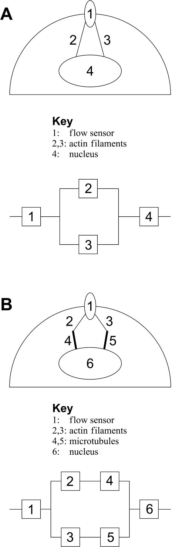
Model networks for endothelial shear stress transmission. (A) Schematic and Kelvin body representation of a four-body network consisting of a flow sensor (body 1) connected to two actin stress fibers (bodies 2 and 3) that are in turn connected to the cell nucleus (body 4). (B) Schematic and Kelvin body representation of a six-body network consisting of a flow sensor (body 1) connected to two actin stress fibers (bodies 2 and 3) that are connected to the nucleus (body 6) via two microtubules (bodies 4 and 5).

The second simulated network (Fig. 3 B) is slightly more complex, and it is inspired by experimental evidence that different components of cytoskeleton are coupled to one another, often via various linker proteins. This network consists of a flow sensor (Kelvin body 1) connected in series to two actin stress fibers (bodies 2 and 3) that are connected in parallel. Each of the stress fibers is subsequently coupled to a microtubule (bodies 4 and 5), and the two microtubules are connected to the cell nucleus (body 6). The corresponding Kelvin body network representation is also shown in Fig. 3 B.

Model parameter values

For each type of viscoelastic body modeled, the values of the two spring constants k₁ and k₂ as well as the dashpot coefficient of viscosity μ must be specified. The baseline values used in the simulations are shown in Table 1. The values for actin filaments are based on micropipette aspiration studies on ECs (Sato et al., 1996). The values for the nucleus are based on recent micropipette aspiration measurements that have demonstrated that the nucleus is three-to-four times stiffer and approximately twice as viscous as the cytoplasm (Guilak et al., 2000). As shown in the Appendix, the parameter values for microtubules were extracted from reports on the relative values of the mechanical properties of microtubules to those of actin filaments. Finally, the parameter values for the Kelvin body representing the flow sensor were based on recent magnetic bead microrheometry data on the mechanical properties of cell-surface integrins (Bausch et al., 1998). As shown in the Appendix, these results had to be recast in a format appropriate for the present analysis. The choice of integrins as the flow sensor in the current analysis is made to simply illustrate the behavior and is not intended to suggest that other cell-surface structures or membrane domains are not involved in flow sensing. Furthermore, it is recognized that the magnetic bead microrheometry measurements do not represent the mechanical properties of integrins alone but will also have a contribution due to cytoskeletal elements to which the integrins are coupled. Within this context, the flow sensor is considered as the transmembrane integrin along with the local cytoskeletal structures that contribute to the measured mechanical behavior.

TABLE 1.

Baseline viscoelastic parameter values used in the simulations

	k1 (Pa)	k2 (Pa)	μ (Pa-s)	Source
Actin filaments	50	100	5000	Sato et al. (1996)
Microtubules	5	10	50,000	Janmey et al. (1991); Davidson et al. (1999)
Integrins	100	200	7.5	Bausch et al. (1999)
Nucleus	200	400	10,000	Guilak et al. (2000)

It should also be noted that an inherent assumption in the present analysis is that the flow sensor is a sufficiently large structure such that the energy imparted to the sensor by the shear stress significantly exceeds the energy associated with the thermal fluctuations of the sensor. This issue was discussed in detail in our previous work (Barakat, 2001) where it was argued that the characteristic dimension of the flow sensor needs to be of order 100 nm for the energy imparted to it by the flow to be an order of magnitude larger than its thermal energy (i.e., ∼10 kT). Structures of this size have indeed been reported to exist within the glycocalyx of ECs (Adamson and Clough, 1992; Feng and Weinbaum, 2000).

In addition to the viscoelastic constants in Table 1, the value of the applied force at t = 0 due to the shear stress is arbitrarily selected as F₀ = 1 (in arbitrary units). The baseline value of the angular frequency in the oscillatory flow simulations is taken as ω = 2π rad/s which corresponds to a physiological cardiac frequency f = 1 Hz (ω = 2πf).

Numerical simulation procedures

The model governing equations were solved numerically using MATLAB. The solution algorithm employed a fourth-order four-stage Runge-Kutta method. The computations were performed on a 600 MHz Pentium-III personal computer with 768 Mbytes of RAM.

RESULTS

Two Kelvin bodies in parallel

Before considering the model EC networks shown in Fig. 3, we will analyze the behavior of a simple configuration consisting of two Kelvin bodies coupled in parallel. This configuration will provide useful insight for the subsequent analyses. Two issues are of specific interest: the force splitting coefficients as the viscoelastic properties of one body change relative to those of the other and differences in overall responses between steady and oscillatory flow stimulation.

We initially consider the two Kelvin bodies to be identical, with each characterized by the baseline parameter values for actin filaments given in Table 1. Fig. 4 A depicts the deformation of each of the two Kelvin bodies as a function of time for both steady and oscillatory flow. Because they are connected in parallel, the deformation is identical in both bodies (Eq. 9). As expected and as described in our previous modeling (Barakat, 2001), the deformation exhibits a step jump upon application of the mechanical force at t = 0 for both steady and oscillatory flow. This deformation is driven by the elastic portion of the viscoelastic behavior (the springs in each Kelvin body), and its magnitude is determined by the initial conditions given in Eq. 19. The immediate deformation response is subsequently followed by gradual creeping toward the long-term asymptotic behavior (which is constant for steady flow and is time periodic for oscillatory flow) as the viscous portion of the response unfolds. As previously shown (Barakat, 2001), the asymptotic response for oscillatory flow is attained virtually instantaneously, while that for steady flow requires considerably longer time (750 s for the deformation to attain 99% of the asymptotic value). Fig. 4 B depicts the evolution of the force in body 1 (F₁(t) = a₁(t)F(t); the force in body 2 will simply be F₂(t) = F(t) − F₁(t)). Not surprisingly, the force divides equally between the two identical bodies under both steady and oscillatory flow conditions. For oscillatory flow, the oscillations in F₁ reflect the periodic oscillation of the imposed force, but the force always divides equally between the two bodies.

FIGURE 4.

(A) Time evolution of the deformation of two identical Kelvin bodies connected in parallel in response to steady and oscillatory flow. Because the evolution to the asymptotic response for the two types of flow occurs over different timescales, oscillatory flow evolution is shown in the inset. For both types of flow, a shear force F₀ is applied at t = 0. Because they are connected in parallel, the two bodies deform equally. The deformation exhibits an instantaneous jump (at t = 0) due to the elastic springs with subsequent creeping as the dashpot deforms. (B) Time evolution of the force in body 1 in response to steady and oscillatory (inset) flow. (C) Peak deformation of the bodies as a function of the applied shear force in response to steady and oscillatory flow.

If the extent of deformation of EC-surface and intracellular structures correlates with the extent of flow-induced cellular signaling, then it is logical that a minimum threshold value of deformation would have to be exceeded to trigger the biological response. Therefore, the magnitude of the peak deformation in response to the two different types of applied flow is of interest. Fig. 4 C illustrates the dependence of this peak deformation on the value of the applied shear force at t = 0 (F₀) for both steady and oscillatory flow for the two-body system. Similar to our previous one-body results (Barakat, 2001), the peak deformation increases linearly with F₀ (i.e., with the applied shear stress). Furthermore, for a given value of F₀, the peak deformation is significantly larger for steady flow than for oscillatory flow.

In a system as complex as a cell, many of the parallel connections are among structures that have drastically different viscoelastic properties. Therefore, we next consider the behavior of the two-body system under both steady and oscillatory flow as the parameter values of Kelvin body 2 are individually varied over a wide range. The parameter values of Kelvin body 1 are held constant at their baseline values (actin values in Table 1). Fig. 5 A depicts the magnitude of the peak deformation of the two-body system as a function of the spring constant k₁₂ for both steady and oscillatory flow. When body 2 is very compliant (k₁₂ small), the peak deformations are largely independent of k₁₂ as the stiffness of the two-body system is entirely dominated by body 1. At intermediate values of k₁₂, the deformations for both steady and oscillatory flow decrease as k₁₂ increases and tend to zero as body 2 becomes very stiff (k₁₂ large). Whereas the peak deformation induced by steady flow is considerably larger than that due to oscillatory flow for relatively compliant structures (small k₁₂), this difference becomes progressively smaller at intermediate k₁₂ values and disappears for very stiff structures (large k₁₂). Fig. 5 B illustrates the peak asymptotic value of F₁ as a function of k₁₂. Peak F₁ exceeds 0.5 for k₁₂ smaller than the baseline value (k₁₂ < 50 Pa), is exactly 0.5 at the baseline value, and falls below 0.5 for k₁₂ > 50. This reflects the fact that a larger fraction of the total applied force gets directed toward the stiffer body, a required condition since the two bodies deform equally.

FIGURE 5.

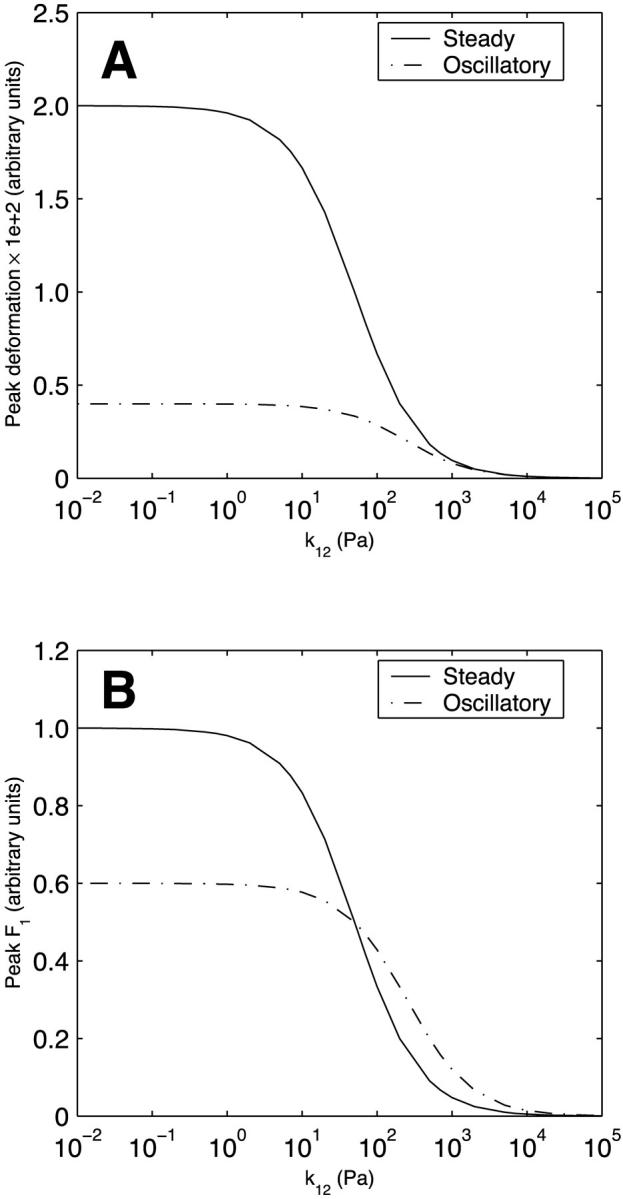
Effect of the spring constant k₁₂ (spring constant of spring 1 in Kelvin body 2) on (A) peak deformation and (B) peak asymptotic force in body 1 in a system of two Kelvin bodies connected in parallel under both steady and oscillatory flow conditions. The remaining constants in the two-body system (k₁₁, k₂₁, μ₁, k₂₂, and μ₂) are assumed constant and are assigned the baseline values of actin (Table 1).

Unlike their dependence on k₁₂, the peak deformation and peak asymptotic F₁ for steady flow are independent of the spring constant k₂₂ (Fig. 6). This is because the impact of the added spring stiffness is compensated for by the dashpot. For oscillatory flow, however, the changes in the forcing function occur over a timescale that is too rapid to allow dashpot compensation; thus, the peak deformation and peak asymptotic F₁, similar to the variations with k₁₂, progressively decrease as k₂₂ increases (Fig. 6). The dependence of peak deformation and peak asymptotic F₁ on the dashpot coefficient of viscosity of body 2 (μ₂) (Fig. 7) largely mirrors that of k₂₂ and can be explained in the same fashion. One difference, however, is that the values do not tend to zero at large μ₂. This is because the spring in series with the dashpot always provides a certain level of compliance. The peak deformation is considerably larger for steady flow than for oscillatory flow over the entire range of k₂₂ and μ₂.

FIGURE 6.

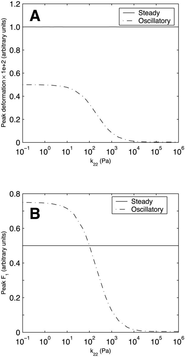
Effect of the spring constant k₂₂ (spring constant of spring 2 in Kelvin body 2) on (A) peak deformation and (B) peak asymptotic force in body 1 in a system of two Kelvin bodies connected in parallel under both steady and oscillatory flow conditions. The remaining constants in the two-body system (k₁₁, k₂₁, μ₁, k₁₂, and μ₂) are assumed constant and are assigned the baseline values of actin (Table 1).

FIGURE 7.

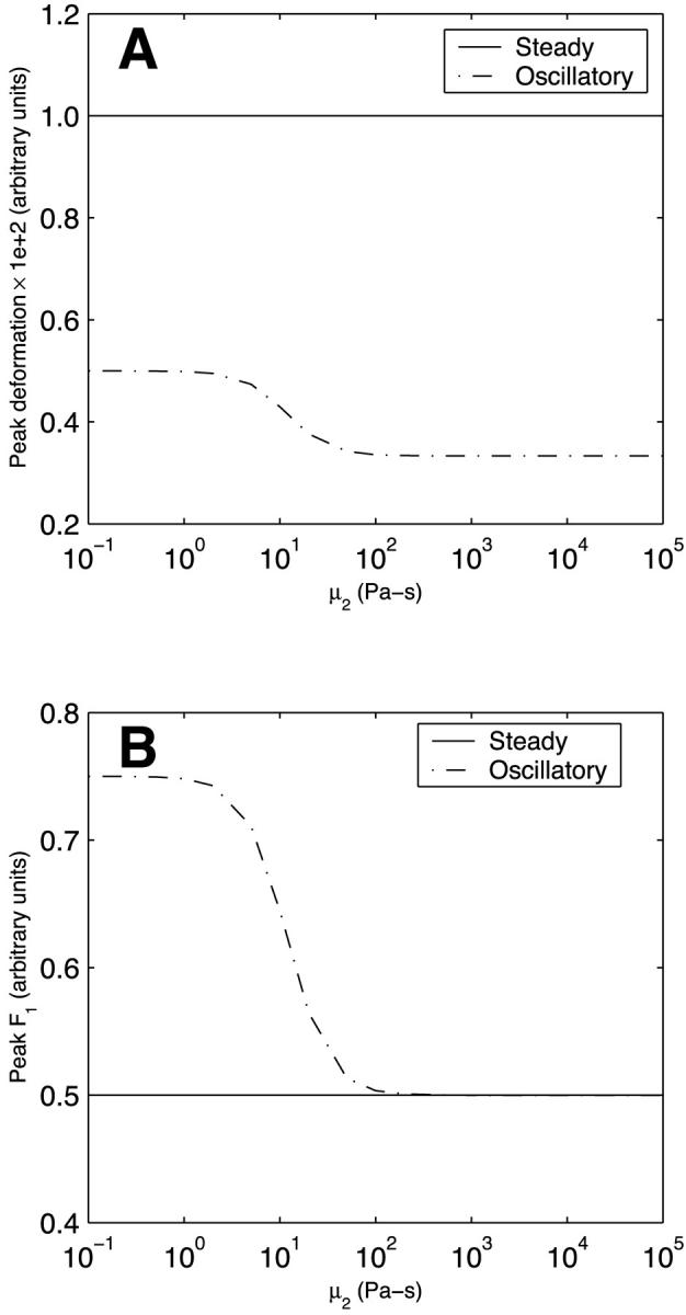
Effect of the dashpot coefficient of viscosity μ₂ of Kelvin body 2 on (A) peak deformation and (B) peak asymptotic force in body 1 in a system of two Kelvin bodies connected in parallel under both steady and oscillatory flow conditions. The remaining constants in the two-body system (k₁₁, k₂₁, μ₁, k₁₂, and k₂₂) are assumed constant and are assigned the baseline values of actin (Table 1).

Figs. 5–7 only considered the dependence of the asymptotic values of the force divisions between the two Kelvin bodies on the viscoelastic properties. It is desirable to probe the evolution of the force division in time to understand how the applied force transiently redistributes between the two bodies. Fig. 8 depicts the evolution of F₁(t) (i.e., a₁(t)F(t)) for steady flow for selected values of k₁₂, k₂₂, and μ₂. At the baseline values of the parameters (those of actin in Table 1), F₁ has the constant value of 0.5 as the two bodies are identical. At other values of k₁₂, F₁ monotonically approaches its asymptotic value given in Fig. 5 B over a period of several hundred seconds (Fig. 8 A). Figs. 6 B and 7 B had demonstrated that the asymptotic value of F₁ for steady flow is independent of k₂₂ and μ₂; however, because the compensation by the dashpot requires time, the transient approach to the asymptotic value does depend on these parameters, and this dependence is not monotonic. For small k₂₂, F₁ is initially large, then decreases below the asymptotic value before increasing until it attains the asymptotic value (Fig. 8 B). For large k₂₂, the opposite occurs—F₁ is initially small, and increases above the asymptotic value before gradually decreasing to the asymptotic value (Fig. 8 B). For small μ₂, F₁ initially increases and then decreases toward the asymptotic value, whereas for large μ₂, F₁ initially decreases to levels considerably below the asymptotic value before increasing to the asymptotic value (Fig. 8 C). These results broadly imply that the force division between the two bodies exhibits prominent transient behavior before attaining its asymptotic value.

FIGURE 8.

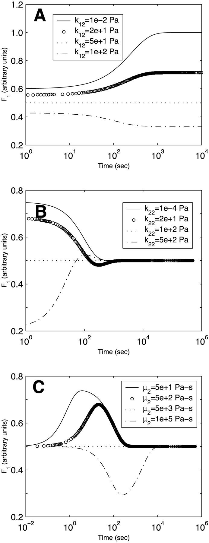
Time evolution of the force in body 1 in a system of two Kelvin bodies connected in parallel and subjected to steady flow. The evolution is shown for selected values of (A) k₁₂, (B) k₂₂, and (C) μ₂. Only the parameter shown is varied. All other parameters are maintained constant at the baseline values of actin (Table 1).

All the oscillatory flow simulations thus far have been performed with a pulsatile frequency f = 1 Hz (ω = 2πf = 2π rad/s), physiological under resting conditions. Under vigorous exercise conditions, this frequency may be considerably higher. Furthermore, certain pathologies have a considerable impact on cardiac frequency. It is expected that as the pulsatile frequency tends to zero, the oscillatory flow behavior would approach that of steady flow. On the other hand, at very high pulsatile frequencies, the inertia of the dashpot of each Kelvin body will prevent it from sensing and responding to the oscillation so that the behavior is dictated entirely by the elastic springs. Because the springs respond instantaneously, the response at very high frequencies would be expected to be independent of frequency. In between these two limits, the deformation would be expected to decrease with frequency as the dashpot has progressively less time to deform. This behavior is confirmed in Fig. 9 A which depicts the peak deformation of the two-body system in oscillatory flow (normalized by the peak deformation under steady flow conditions) as a function of the pulsatile frequency for different values of the coefficient viscosity of body 2 (μ₂). For all values of μ₂, the normalized peak deformation tends to unity at very small frequencies. As the oscillatory frequency increases, the behavior depends on the value of μ₂. For most values of μ₂ considered, the behavior is sigmoidal with a critical frequency of ∼0.01–0.1 Hz (depending on μ₂) above which the peak deformation becomes frequency-independent. Interestingly, for very small μ₂, the behavior becomes bi-sigmoidal. This reflects the fact that a less viscous dashpot can respond to considerably higher oscillation frequencies.

FIGURE 9.

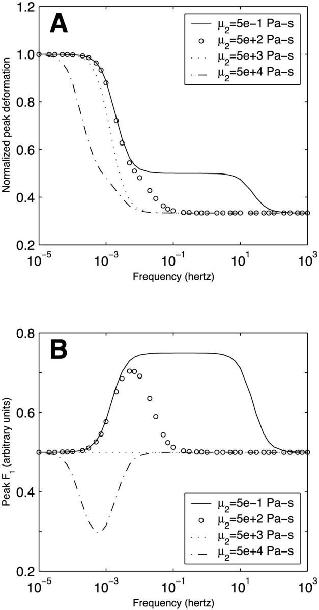
Dependence of (A) peak long-term deformation and (B) peak asymptotic force division on frequency in a system of two Kelvin bodies connected in parallel and subjected to oscillatory flow. The results are shown for different values of body 2 dashpot coefficient of viscosity μ₂. The deformations have been normalized by the steady state value for steady flow.

Fig. 9 B illustrates the magnitude of the peak asymptotic F₁ for oscillatory flow as a function of the applied oscillatory frequency for different values of μ₂. Not surprisingly, the results demonstrate frequency sensitivity only over a particular frequency range. For μ₂ < μ₁ (μ₁ is held constant at 5000 Pa-s), more of the applied force needs to go into body 1 to elicit a deformation equal to that of body 2; therefore, F₁ exceeds 0.5. The opposite occurs for μ₂ > μ₁. At sufficiently large frequencies, the dashpots become nonresponsive, and the force division becomes entirely dictated by the springs. At very small frequencies, oscillatory flow approaches steady flow. In both limits, the applied force divides equally between the two bodies (i.e., F₁ = 0.5).

Model EC networks

We now consider the two simple EC networks depicted in Fig. 3. Fig. 10 A illustrates the evolution of the deformations of each component of the four-body network in Fig. 3 A in response to steady flow. All four bodies qualitatively exhibit the typical pattern of an instantaneous deformation followed by gradual creeping (compare to Fig. 4 A); however, there are differences among the different structures. Because of its very small dashpot coefficient of viscosity, the transmembrane integrin (flow sensor) attains its peak deformation much more rapidly than the other structures. The two actin stress fibers deform slowly but ultimately attain a peak deformation equivalent to that of the transmembrane protein. Because they are connected in parallel, the two stress fibers deform equally. The fact that the asymptotic stress fiber deformation is equal to that of the flow sensor reflects the fact that this deformation for each structure is dictated by the spring constant k₂, and the value of k₂ for the flow sensor is twice that of each of the two stress fibers (Table 1). Finally, the nucleus attains its peak deformation with a characteristic time constant that is considerably slower than that of the transmembrane protein but two–three times faster than that of the stress fibers; however, this peak deformation is only half that of the other structures (since (k₂)_nucleus = 2(k₂)_integrins (Table 1)). As shown in Fig. 10 B, the flow sensor, actin filaments, and nucleus in the six-body network of Fig. 3 B deform identically to the case of the four-body network. The microtubules exhibit considerably slower deformation due to the large coefficient of viscosity; however, the amplitude of their asymptotic deformation is large due to the small value of (k₂)_microtubules (Table 1). Interestingly, the time constants observed in the simulations are broadly consistent with the experimental observations that when ECs are exposed to steady flow, candidate flow sensors such as flow-sensitive ion channels and cell-surface integrins respond very rapidly (milliseconds to seconds), the nuclear responses exhibit intermediate timescales (minutes to a few hours), while the cytoskeletal remodeling is not complete until many hours after the onset of flow (Davies, 1995).

FIGURE 10.

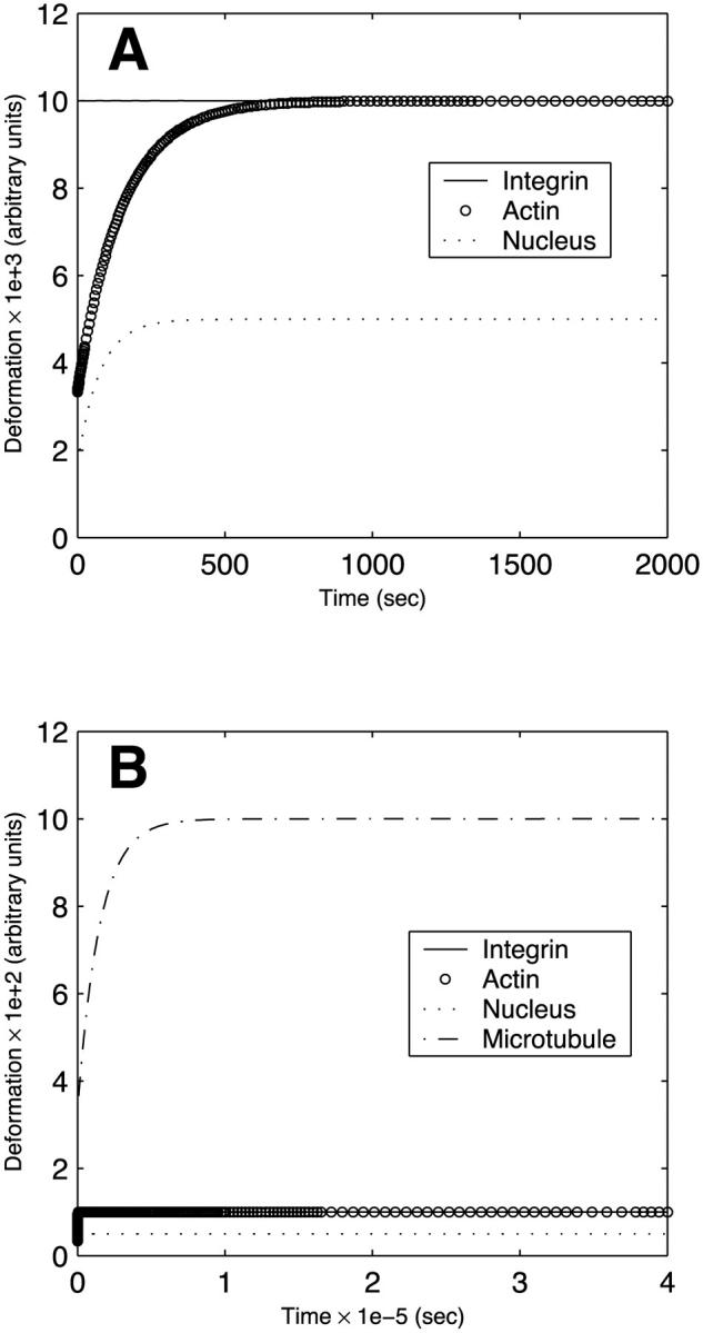
Time evolution of the deformation of each component of model endothelial networks under steady flow conditions. (A) Four-body network depicted in Fig. 3 A. (B) Six-body network depicted in Fig. 3 B.

Fig. 11 depicts the dependence of the peak asymptotic deformation of each structure in the six-body network of Fig. 3 B on the driving frequency under oscillatory flow conditions. Similar to the behavior discussed previously (Fig. 9 A), the deformations of all bodies approach the asymptotic steady flow values of Fig. 10 B for small frequencies and become independent of frequency at high frequencies. Significantly, at a physiological frequency of 1 Hz, the deformation of each of the network components is considerably smaller in oscillatory flow than in steady flow.

FIGURE 11.

Dependence of the peak asymptotic deformation of each component of the six-body model endothelial network depicted in Fig. 3 B on the frequency under oscillatory flow conditions.

DISCUSSION

Endothelial responsiveness to fluid mechanical stimulation may involve the sensing of the stimulus at the cell surface and its subsequent transmission by cytoskeletal elements to various intracellular transduction sites. Although the mechanisms of mechanosensing and transmission remain to be elucidated, direct deformation of cell-surface and intracellular structures may be involved (Davies and Tripathi, 1993; Davies, 1995). In this article, we have formulated a simple model of mechanical signal transmission in ECs by considering the transmission pathways as networks of coupled viscoelastic bodies that deform in response to an applied mechanical force. The viscoelastic response is simulated as a standard linear solid (Kelvin body). Because steady and oscillatory flow induce different biological responses in ECs (Helmlinger et al., 1991, 1995; Chappell et al., 1998; Lum et al., 2000; Suvatne et al., 2001), we have focused on differences in the deformations of the individual components of these networks in response to steady and oscillatory flow. Moreover, we have investigated the sensitivity of the resulting deformations to various model parameters including the spring constants, the dashpot coefficient of viscosity, and the oscillatory flow frequency.

As an example of a very simple network, we initially considered two Kelvin bodies connected in parallel. When this network was subjected to steady flow, both bodies underwent an instantaneous deformation due to the elastic springs; this deformation was subsequently followed by gradual creeping toward the long-term response. When the flow was oscillatory, the deformation also oscillated with the driving force, and the long-term time-periodic behavior was attained very rapidly. When the two bodies had identical viscoelastic properties, the applied force expectedly divided equally between them. Making one of the bodies stiffer reduced the magnitude of the flow-induced deformation of both bodies and shifted the force division in favor of the stiffer body. This shift was needed because a larger force needs to be applied to a stiffer body than to a more compliant one if the two bodies are to deform equally.

Our results have also demonstrated that the transient approach of the force division between the two bodies toward its asymptotic value is not necessarily monotonic. In an EC, this suggests that depending on the time point after initiation of flow, the force division between two intracellular structures connected in parallel may be transiently in favor of one of the structures or the other. If a minimum threshold force needs to be exceeded to initiate signaling associated with a particular intracellular structure, then these results suggest that certain signaling pathways are activated for only a limited time period after flow onset. This may reflect a form of signal desensitization and/or adaptation. Indeed, experiments have demonstrated that a number of endothelial flow responses including Ca²⁺ oscillations and transcriptional changes of certain flow-responsive genes are transient in nature (Shen et al., 1992; Resnick and Gimbrone, 1995).

While steady flow induces mobilization of intracellular Ca²⁺ and reorganization of cytoskeleton in ECs, purely oscillatory flow with a physiological oscillation frequency of 1 Hz does not induce either response (Helmlinger et al., 1991, 1995). Furthermore, some of the transcriptional changes induced by steady flow do not occur in response to 1-Hz oscillatory flow (Suvatne et al., 2001). The mechanisms by which ECs distinguish among and respond differently to different types of flow remain unknown. Our model results have demonstrated that steady flow generally induces larger deformations than 1-Hz oscillatory flow. If the intensity of flow-induced endothelial signaling depends on the extent of deformation of cell-surface and intracellular structures, then our results may provide insight into mechanisms governing experimentally observed differences between steady and oscillatory flow responses.

The differences in deformation of cell-surface and intracellular structures between steady and 1-Hz oscillatory flow disappear when the frequency of oscillation becomes sufficiently small. This behavior is not surprising since in the limit of very low frequency, oscillatory flow tends to steady flow. These results suggest that EC responses induced by steady flow but not by 1-Hz oscillatory flow will develop if the oscillatory flow experiments were performed at sufficiently low frequencies. Our analysis also demonstrates that at very high oscillation frequencies, the magnitude of flow-induced deformation becomes independent of frequency. These model predictions are directly testable experimentally.

Two types of multibody networks were analyzed to model transmission of the flow stimulus from the luminal cell surface to the nucleus in ECs. The first was a four-body network consisting of a cell-surface flow sensor coupled to two actin stress fibers that are in turn coupled to the nucleus. The second network was a six-body network consisting of a cell-surface sensor connected to two stress fibers each of which was directly connected to a microtubule. The two microtubules subsequently coupled directly to the nucleus. Simulations of these simple networks demonstrated that the cell-surface structure attains its peak deformation much faster than the intracellular structures. The nucleus deforms more rapidly than the cytoskeletal elements, but because of its high stiffness, its peak deformation is relatively small. These relative time constants are consistent with the experimentally observed temporal chronology of EC flow responses: candidate flow sensors such as flow-sensitive ion channels and cell-surface integrins respond very rapidly (milliseconds to seconds), gene and protein regulatory responses occur over intermediate timescales (minutes to a few hours), while cytoskeletal and morphological reorganization is not fully attained until many hours after flow initiation (Davies, 1995). Although only very simple networks have been presented in the illustrative examples in this article, arbitrarily complex networks can be analyzed using the same formulation as long as these networks can be reduced into sets of bodies connected in combinations of series and/or parallel configurations.

Recent studies have demonstrated a rapid increase in EC membrane fluidity upon initiation of flow (Haidekker et al., 2000; Butler et al., 2001); this has led to the suggestion that the cell membrane as a whole may act as a flow sensor. Although the current presentation has focused on discrete cell-surface structures as candidate flow sensors, the same analysis can be used had the cell membrane itself been considered as the flow sensor. The only difference in that case would be that appropriate viscoelastic properties of lipid bilayers would need to be used in lieu of those that characterize specific cell-surface structures.

Our results have their most direct implications to EC flow signaling if the intensity of this signaling correlates with the extent of mechanical deformation of various cell-surface and intracellular structures. It is recognized that this may not be the case for all types of EC flow responses. For instance, previous mathematical modeling of the impact of fluid mechanical shear stress on intracellular calcium concentration in which both the effect of flow on the delivery of calcium agonists to the EC surface and the impact of flow-induced cell membrane strain on the open probability of calcium channels have been included has demonstrated that the calcium response to flow depends on the relative dynamics of the biochemical steps involved in calcium mobilization and is not simply proportional to the magnitude of flow-induced membrane strain (Wiesner et al., 1997). It is envisioned that there exists a range of flow conditions where the mechanical strain kinetics constitute the dominant contribution to signaling, and it is in this range that our present results are most applicable. It should also be noted that the mechanical form of signaling modeled here is considered complementary to, rather than a substitute for, more well characterized receptor-mediated signal transduction pathways.

Micropipette aspiration studies on cultured ECs have demonstrated that these cells become considerably stiffer upon flow exposure (Sato et al., 1996). This suggests that the viscoelastic parameters used in the modeling should most generally be considered time-dependent. Furthermore, the various components of the cytoskeleton are connected together and to other cell structures via a variety of linker proteins whose viscoelastic properties likely impact the overall flow-induced deformations. Unfortunately, no data currently exist on the mechanical properties of these linker proteins, so their effect cannot be realistically incorporated. Finally, a number of staining studies have demonstrated that cellular cytoskeleton consists of very dense and complex networks that likely cannot always be reduced to simple configurations of structures connected in series and/or parallel; therefore, it would be important to generalize the present results to arbitrarily structured networks. Data from various fields including network theory and pattern recognition promise to be very useful in this regard.

APPENDIX

Model parameter values for cell-surface flow sensor

As mentioned in the text, the parameter values for the flow sensor on the EC surface were derived from recent magnetic bead microrheometry measurements of the viscoelastic properties of integrins (Bausch et al., 1998). As also noted in the text, these measurements likely contain a contribution from local cytoskeletal elements to which the integrins are coupled. It is impossible at this point to isolate the effects of integrins from those of local cytoskeleton; therefore, the flow sensor is considered to consist of the complex of integrins and the local cytoskeletal structures to which these integrins are directly coupled. In the study by Bausch and co-workers (Bausch et al., 1998), study, the values of the spring constants had the dimensions of Pa-m while the dashpot coefficient of viscosity had the dimensions of Pa-m-s. In contrast, the spring constants and the coefficient of viscosity for actin and the nucleus given by other investigators were respectively in Pa and Pa-s (Sato et al., 1996, and Guilak et al., 2000). Fundamentally, the difference is due to the method by which the viscoelastic parameters were derived. The micropipette aspiration experiments of Sato et al. (1996) and Guilak et al. (2000) applied a given pressure difference and measured the resulting deformation, while the magnetic bead microrheometry measurements involved the application of a known twisting force and measuring the resulting deformation. For the parameter values in our model to be consistent, we have to recast the values obtained by Bausch et al. (1998) in terms of the dimensions given by Sato et al. (1996) and Guilak et al. (2000).

Sato et al. (1996) modeled the viscoelastic behavior describing their micropipette aspiration data using a Kelvin body for which the measurements were fit to the function

(A1)

where L is the measured deformation [m], Δp is the applied pressure difference [Pa], a is the micropipette diameter [m], and τ is the time constant associated with the deformation [s]. The spring constants k₁ and k₂ have the dimensions of Pa.

On the other hand, Bausch et al. (1998) modeled their magnetic bead microrheometry results using a viscoelastic model consisting of a Kelvin body in series with a dashpot, and they demonstrated that this circuit captures the experimentally observed triphasic creep response consisting of an elastic domain, a relaxation regime, and a viscous flow domain. For this system, the equivalent expression to Eq. A1 is

(A2)

where F is the applied twisting force [N], k₁ and k₂ are the spring constants associated with the Kelvin body [Pa-m], μ_d is the coefficient of viscosity of the dashpot [Pa-s-m], and τ is the relaxation time [s] of the Kelvin body given by:

(A3)

where μ is the Kelvin body's coefficient of viscosity [Pa-s-m]. The first term in Eq. A2 corresponds to the deformation of the Kelvin body, whereas the second term corresponds to the deformation of the dashpot.

To recast the spring constants derived by Bausch et al. (1998) in equivalent terms to those of Sato et al. (1996), we determine the applied force in the study of Sato et al. (1996) due to the pressure difference Δp. This force is given by F = Δpπa² ∼ 2500 pN. From Eq. A2, the initial deformation at t = 0 is given by

(A4)

For the Kelvin body portion in Eq. A2, the deformation at steady state (as t → ∞) is given by

(A5)

Eqs. A4 and A5, when applied to the force and deformation data of Sato et al. (1996), can be used to obtain values for the spring constants k₁ and k₂ in dimensions that match those given by Bausch et al. (1998). This calculation yields k₁ = 6.25 × 10⁻⁴ Pa-m and k₂ = 9.38 × 10⁻⁴ Pa-m.

Similar computations need to be performed on the data of Bausch et al. (1998) to derive properties for the flow sensor (integrins plus coupled local cytoskeleton). Because in the steady state (as t → ∞) the deformation given in Eq. A2 leads to a linear variation with time, the parameter values used in the present manuscript are derived from within the linear regime, i.e., after the Kelvin body had attained its steady-state behavior. For an applied force of ∼2000 pN (comparable to the force applied in Sato et al., 1996), Bausch et al. (1998) measured initial and steady state deformations per unit force of ∼350 m/N and ∼800 m/N, so that the initial and steady-state deformations were respectively L₀ ∼ 7 × 10⁻⁷ m and L_s ∼ 1.6 × 10⁻⁶ m. Substituting these values into Eqs. A4 and A5 leads to k₁ ∼ 1.25 × 10⁻³ Pa-m and k₂ ∼ 1.61 × 10⁻³ Pa-m. These are the values of the spring constants for the flow sensor.

Finally, we must obtain the coefficient of viscosity of the dashpot of the Kelvin body (μ) for both Sato et al. (1996) and Bausch et al. (1998). μ is related to the spring constants as shown in Eq. A3. In Sato et al. (1996), τ for cytoskeleton has a value of ∼110 s so that μ = 4.125 × 10⁻² Pa-m-s, whereas in Bausch et al. (1998), τ for integrins has a value of ∼0.09 s so that μ = 6.33 × 10⁻⁵ Pa-m-s.

Now that the parameter values in the two studies have been expressed in similar dimensions, they can be directly compared. k₁ and k₂ for the cell-surface integrins are approximately twice their values for actin filaments, and the coefficient of viscosity of integrins is approximately 1.5 × 10⁻³ that of actin filaments. Therefore, recasting the integrin parameters in terms of the dimensions given by Sato et al. (1996) yields k₁ ≅ 2(50 Pa) = 100 Pa, k₂ ≅ 2(100 Pa) = 200 Pa, and μ ≅ (1.5 × 10⁻³)(5000 Pa-s) = 7.5 Pa-s. These are the flow sensor parameter values given in Table 1.

Model parameter values for microtubules

For a Kelvin body, the magnitude of the instantaneous deformation at t = 0 upon application of a force F is given by F/(k₁ + k₂), whereas the long-term deformation is given by F/k₁ (Eqs. A4 and A5). Using the long-term deformation data of Janmey et al. (1991) for both actin filaments and microtubules and combining this information with the data of Davidson et al. (1999), we obtain a ratio of k₂ for actin to that of microtubules of ∼36. Given that (k₂)_actin = 100 Pa, we obtain (k₂)_microtubules ≅ 2.8 Pa. As shown in Table 1, we use a value of (k₂)_microtubules = 5 Pa in the simulations. The same experimental data can be used to determine that the ratio of (k₁ + k₂) for actin to that for microtubules is ∼15. Given that (k₁)_actin = 50 Pa, (k₂)_actin = 100 Pa, and (k₂)_microtubules ≅ 2.8 Pa, we obtain a value of (k₁)_microtubules ≅ 7.2 Pa. We use a value of (k₁)_microtubules = 10 Pa in the simulations (Table 1). Finally, as given in Eq. A3, μ_microtubules can be determined if the ratio of the time constants associated with the deformation of microtubules and actin filaments (τ_microtubules/τ_actin) is known. From the data of Davidson et al. (1999), we estimate this ratio to be ∼180. Given the values of k₁ and k₂ for both actin and microtubules and the value of μ_actin = 5000 Pa-s, we determine that μ_microtubules ∼ 57,000 Pa-s. We use a value of μ_microtubules = 50,000 Pa-s in the simulations (Table 1). The parameter values derived for microtubules are consistent with the qualitative observation that microtubules are considerably less rigid than actin filaments (Janmey et al., 1991).

References

- Ando, J., T. Komatsude, and A. Kamiya. 1988. Cytoplasmic calcium responses to fluid shear stress in cultured vascular endothelial cells. In Vitro Cell. Dev. Biol. 24:871–877. [DOI] [PubMed] [Google Scholar]
- Adamson, R. H., and G. Clough. 1992. Plasma proteins modify the endothelial cell glycocalyx of frog mesenteric microvessels. J. Physiol. 445:473–486. [DOI] [PMC free article] [PubMed] [Google Scholar]
- Asakura, T., and T. Karino. 1990. Flow patterns and spatial distribution of atherosclerotic lesions in human coronary arteries. Circ. Res. 66:1045–1066. [DOI] [PubMed] [Google Scholar]
- Barakat, A. I. 2001. A model for shear stress-induced deformation of a flow sensor on the surface of vascular endothelial cells. J. Theor. Biol. 210:221–236. [DOI] [PubMed] [Google Scholar]
- Barakat, A. I., E. V. Leaver, P. A. Pappone, and P. F. Davies. 1999. A flow-activated chloride-selective membrane current in vascular endothelial cells. Circ. Res. 85:820–828. [DOI] [PubMed] [Google Scholar]
- Bausch, A. R., F. Ziemann, A. A. Boulbitch, K. Jacobson, and E. Sackmann. 1998. Local measurements of viscoelastic parameters of adherent cell surfaces by magnetic bead microrheometry. Biophys. J. 75:2038–2049. [DOI] [PMC free article] [PubMed] [Google Scholar]
- Butler, P. J., G. Norwich, S. Weinbaum, and S. Chien. 2001. Shear stress induces a time- and position-dependent increase in endothelial cell membrane fluidity. Am. J. Physiol. 280:C962–C969. [DOI] [PubMed] [Google Scholar]
- Chappell, D. C., S. E. Varner, R. M. Nerem, R. M. Medford, and R. W. Alexander. 1998. Oscillatory shear stress stimulates adhesion molecule expression in cultured human endothelium. Circ. Res. 82:532–539. [DOI] [PubMed] [Google Scholar]
- Critchley, D. R. 2000. Focal adhesions—the cytoskeletal connection. Curr. Opin. Cell Biol. 12:133–139. [DOI] [PubMed] [Google Scholar]
- Davidson, L. A., G. F. Oster, R. E. Keller, and M. A. Koehl. 1999. Measurements of mechanical properties of the blastula wall reveal which hypothesized mechanisms of primary invagination are physically plausible in the sea urchin Strongylocentrotus purpuratus. Dev. Biol. 209:221–238. [DOI] [PubMed] [Google Scholar]
- Davies, P. F. 1995. Flow-mediated endothelial mechanotransduction. Physiol. Rev. 75:519–560. [DOI] [PMC free article] [PubMed] [Google Scholar]
- Davies, P. F., and S. C. Tripathi. 1993. Mechanical stress mechanisms and the cell: an endothelial paradigm. Circ. Res. 72:239–245. [DOI] [PubMed] [Google Scholar]
- Dewey, C. F., Jr., S. R. Bussolari, M. A. Gimbrone, Jr., and P. F. Davies. 1981. The dynamic response of vascular endothelial cells to fluid shear stress. J. Biomech. Eng. 103:177–188. [DOI] [PubMed] [Google Scholar]
- Dull, R. O., and P. F. Davies. 1991. Flow modulation of agonist (ATP)-response (Ca2+) coupling in vascular endothelial cells. Am. J. Physiol. 261:H149–H156. [DOI] [PubMed] [Google Scholar]
- Eskin, S. G., C. L. Ives, L. V. McIntire, and L. T. Navarro. 1984. Response of cultured endothelial cells to steady flow. Microvasc. Res. 28:87–93. [DOI] [PubMed] [Google Scholar]
- Feng, J., and S. Weinbaum. 2000. Lubrication theory in highly compressible porous media: the mechanics of skiing, from red cells to humans. J. Fluid Mech. 422:281–317. [Google Scholar]
- Fung, Y. C. 1981. Biomechanics: Mechanical Properties of Living Tissues. Springer-Verlag, New York.
- Garcia-Cardena, G., J. Comander, K. R. Anderson, B. R. Blackman, and M. A. Gimbrone, Jr. 2001. Biomechanical activation of vascular endothelium as a determinant of its functional phenotype. Proc. Natl. Acad. Sci. USA. 98:4478–4485. [DOI] [PMC free article] [PubMed] [Google Scholar]
- Geiger, R. V., B. C. Berk, R. W. Alexander, and R. M. Nerem. 1992. Flow-induced calcium transients in single endothelial cells: spatial and temporal analysis. Am. J. Physiol. 262:C1411–C1417. [DOI] [PubMed] [Google Scholar]
- Gudi, S. R. P., C. B. Clark, and J. A. Frangos. 1996. Fluid flow rapidly activates G-proteins in human endothelial cells: involvement of G-proteins in mechanochemical signal transduction. Circ. Res. 79:834–839. [DOI] [PubMed] [Google Scholar]
- Gudi, S., J. P. Nolan, and J. A. Frangos. 1998. Modulation of GTPase activity of G-proteins by fluid shear stress and phospholipid composition. Proc. Natl. Acad. Sci. USA. 95:2515–2519. [DOI] [PMC free article] [PubMed] [Google Scholar]
- Guilak, F., J. R. Tedrow, and R. Burgkart. 2000. Viscoelastic properties of the cell nucleus. Biochem. Biophys. Res. Comm. 269:781–786. [DOI] [PubMed] [Google Scholar]
- Haidekker, M. A., N. L'Heureux, and J. A. Frangos. 2000. Fluid shear stress increases membrane fluidity in endothelial cells: a study with DCVJ fluorescence. Am. J. Physiol. 278:H1401–H1406. [DOI] [PubMed] [Google Scholar]
- Helmlinger, G., R. V. Geiger, S. Schreck, and R. M. Nerem. 1991. Effects of pulsatile flow on cultured vascular endothelial cell morphology. J. Biomech. Eng. 113:123–134. [DOI] [PubMed] [Google Scholar]
- Helmlinger, G., B. C. Berk, and R. M. Nerem. 1995. Calcium responses of endothelial cell monolayers subjected to pulsatile and steady laminar flow differ. Am. J. Physiol. 269:C367–C375. [DOI] [PubMed] [Google Scholar]
- Ingber, D. E. 1993. Cellular tensegrity: defining new rules of biological design that govern the cytoskeleton. J. Cell Sci. 104:613–627. [DOI] [PubMed] [Google Scholar]
- Ingber, D. E., L. Dike, L. Hansen, S. Karp, H. Liley, A. Maniotis, H. McNamee, D. Mooney, G. Plopper, J. Sims, and N. Wang. 1994. Cellular tensegrity: exploring how mechanical changes in the cytoskeleton regulate cell growth, migration, and tissue pattern during morphogenesis. Int. Rev. Cytol. 150:173–224. [DOI] [PubMed] [Google Scholar]
- Jacobs, E. R., C. Cheliakin, D. Gebremedhin, P. F. Davies, and D. R. Harder. 1995. Shear activated channels in cell-attached patches of cultured bovine aortic endothelial cells. Pflug. Arch. 431:129–131. [DOI] [PubMed] [Google Scholar]
- Janmey, P. A., U. Euteneuer, P. Traub, and M. Schliwa. 1991. Viscoelastic properties of vimentin compared with other filamentous biopolymer networks. J. Cell Biol. 113:155–160. [DOI] [PMC free article] [PubMed] [Google Scholar]
- Ku, D. N., D. P. Giddens, C. K. Zarins, and S. Glagov. 1985. Pulsatile flow and atherosclerosis in the human carotid bifurcation. Positive correlation between plaque location and low and oscillating shear stress. Arteriosclerosis. 5:293–302. [DOI] [PubMed] [Google Scholar]
- Langille, B. L., and F. O'Donnell. 1986. Reductions in arterial diameter produced by chronic decreases in blood flow are endothelium-dependent. Science. 231:405–407. [DOI] [PubMed] [Google Scholar]
- Lum, R. M., L. M. Wiley, and A. I. Barakat. 2000. Influence of different forms of shear stress on vascular endothelial TGF-β1 mRNA expression. Int. J. Mol. Med. 5:635–641. [DOI] [PubMed] [Google Scholar]
- Malek, A. M., and S. Izumo. 1994. Molecular Aspects of Signal Transduction of Shear Stress in the Endothelial Cell. J. Hypertens. 12:989–999. [PubMed] [Google Scholar]
- Nakao, M., K. Ono, F. Fujisawa, and T. Iijima. 1999. Mechanical stress-induced Ca2+ entry and Cl− current in cultured human aortic endothelial cells. Am. J. Physiol. 276:C238–C249. [DOI] [PubMed] [Google Scholar]
- Nerem, R. M., M. J. Levesque, and J. F. Cornhill. 1981. Vascular endothelial morphology as an indicator of the pattern of blood flow. J. Biomech. Eng. 103:172–177. [DOI] [PubMed] [Google Scholar]
- Nerem, R. M. 1992. Vascular fluid mechanics, the arterial wall, and atherosclerosis. J. Biomech. Eng. 114:274–282. [DOI] [PubMed] [Google Scholar]
- Olesen, S. P., D. E. Clapham, and P. F. Davies. 1988. Hemodynamic shear stress activates a K+ current in vascular endothelial cells. Nature. 331:168–170. [DOI] [PubMed] [Google Scholar]
- Pohl, U., J. Holtz, R. Busse, and E. Bassenge. 1986. Crucial role of endothelium in the vasodilator response to increased flow in vivo. Hypertension. 8:37–47. [DOI] [PubMed] [Google Scholar]
- Resnick, N., and M. A. Gimbrone, Jr. 1995. Hemodynamic forces are complex regulators of endothelial gene expression. FASEB J. 9:874–882. [DOI] [PubMed] [Google Scholar]
- Sato, M., N. Ohshima, and R. M. Nerem. 1996. Viscoelastic properties of cultured porcine aortic endothelial cells exposed to shear stress. J. Biomech. 29:461–467. [DOI] [PubMed] [Google Scholar]
- Shen, J., F. W. Luscinskas, A. Connolly, C. F. Dewey, Jr., and M. A. Gimbrone, Jr. 1992. Fluid shear stress modulates cytosolic free calcium in vascular endothelial cells. Am. J. Physiol. 262:C384–C390. [DOI] [PubMed] [Google Scholar]
- Suvatne, J., A. I. Barakat, and M. E. O'Donnell. 2001. Flow-induced expression of endothelial Na-K-Cl cotransport: dependence on K+ and Cl− channels. Am. J. Physiol. 280:C216–C227. [DOI] [PubMed] [Google Scholar]
- Traub, O., and B. C. Berk. 1998. Laminar shear stress—mechanisms by which endothelial cells transduce an atheroprotective force. Arterioscler. Thromb. Vasc. Biol. 18:677–685. [DOI] [PubMed] [Google Scholar]
- Wiesner, T. F., B. C. Berk, and R. M. Nerem. 1997. A mathematical model of the cytosolic-free calcium response in endothelial cells to fluid shear stress. Proc. Natl. Acad. Sci. USA. 94:3726–3731. [DOI] [PMC free article] [PubMed] [Google Scholar]
- Zamir, E., and B. Geiger. 2001. Molecular complexity and dynamics of cell-matrix adhesions. J. Cell Sci. 114:3583–3590. [DOI] [PubMed] [Google Scholar]
- Ziegelstein, R. C., L. Cheng, and M. C. Capogrossi. 1992. Flow dependent cytosolic acidification of vascular endothelial cells. Science. 258:656–659. [DOI] [PubMed] [Google Scholar]