

Abstract
Changes in excluded volume and contact interaction with the surface of a protein have been suggested as mechanisms for the changes in stability induced by cosolvents. The aim of the present paper is to present an analysis that combines both effects in a quantitative manner. The result is that both processes are present in both stabilizing and destabilizing interactions and neither can be ignored. Excluded volume was estimated using accessible surface area calculations of the kind introduced by Lee and Richards. The change in excluded volume on unfolding, ΔX, is quite large. For example, ΔX for ribonuclease is 6.7 L in urea and ∼16 L in sucrose. The latter number is greater than the molar volume of the protein. Direct interaction with the protein is represented as the solvent exchange mechanism, which differs from ordinary association theory because of the weakness of the interaction and the high concentrations of cosolvents. The balance between the two effects and their contribution to overall stability are most simply presented as bar diagrams as in Fig. 3. Our finding for five proteins is that excluded volume contributes to the stabilization of the native structure and that contact interaction contributes to destabilization. This is true for five proteins and four cosolvents including both denaturants and osmolytes. Whether a substance stabilizes a protein or destabilizes it depends on the relative size of these two contributions. The constant for the cosolvent contact with the protein is remarkably uniform for four of the proteins, indicating a similarity of groups exposed during unfolding. One protein, staphylococcus nuclease, is anomalous in almost all respects. In general, the strength of the interaction with guanidinium is about twice that of urea, which is about twice that of trimethylamine-N-oxide and sucrose. Arguments are presented for the use of volume fractions in equilibrium equations and the ignoring of activity coefficients of the cosolvent. It is shown in the Appendix that both the excluded volume and the direct interaction can be extracted in a unified way from the McMillan-Mayer formula for the second virial coefficient.
INTRODUCTION
The unfolding of proteins by reagents such as urea or guanidinium chloride has long been considered to arise because of the favorable interaction of these reagents with the normally buried interior segments of a protein, thereby stabilizing the unfolded form relative to the folded one (Wu, 1931). In like manner the stabilization of folded protein structures by osmolytes such as sucrose is thought to result from unfavorable interactions with interior residues of the proteins thereby producing a relative destabilization of the unfolded form (Lee and Timasheff, 1981). It is possible to treat both of the above processes as two aspects of the same phenomenon, differing from one another only in the sign of the free energy of interaction (Schellman, 1990). The analogy with Flory's discussion of “good” and “bad” solvents is strong (Flory, 1953). The main difference is that proteins collapse into predesigned three-dimensional structures rather than random aggregates. Water itself is a slightly bad solvent. This is nature's way of causing proteins to fold spontaneously.
A number of different models have been proposed to put this problem into quantitative form. These include: the summation of free energies of transfer of protein groups from solvent to the interior of proteins (Nozaki and Tanford, 1963; Tanford, 1970), changes in solvent surface tension and its effect on exposed protein surface (Arakawa and Timasheff, 1982; Kita et al., 1994), and the correlation of exposed surface area with free energies of exposure (Myers et al., 1995; Baskakov and Bolen, 1999; Courtenay et al., 2000), i.e., “m values” and models in which the solvation region is treated as a domain amenable to thermodynamic analysis (Eisenberg, 1976; Lee and Timasheff, 1974; Courtenay et al., 2001). In recent years, exposed areas have been partitioned into polar and nonpolar parts making use of structural data for the proteins (Pace, 2001).
This paper will deal with a quite old model that attempts to describe the effect of denaturants in terms of basic molecular events: a water molecule in contact with a protein is replaced by a denaturant or osmolyte. Simple equilibrium theory is used, though it takes an unusual form because of the smallness of the binding constants and the high concentrations of denaturant or osmolyte (Schellman, 1987). Section 2, “Physical Aspects of the Model”, provides a description of the physical processes and concepts that are involved in protein-solvent interactions. Section 3, “Formula for Data Analysis”, will combine these processes into a formulation that differs from previous work by the author. Section 4, “Calculation Strategy”, outlines the steps and parameters that are used in the calculations. Section 5, “Excluded Volume and Accessible Area”, discusses the special problem of the excluded volume of unfolded states. Section 6, “Results”, presents the results of calculation on several protein-denaturant and osmolyte systems.
PHYSICAL ASPECTS OF THE MODEL
There has been some misinterpretation of my earlier papers that might be cleared up by a description of the binding event in the context of the site-binding model. As depicted in Fig. 1, the protein molecule is surrounded by water molecules represented by small circles. Most water molecules are not localized on the surface of a protein so that the entire array of contact molecules should be considered as sliding and exchanging in every possible way, the only rule being that the surface must at all times be completely covered. (Kuhn et al. (1992) have made an extensive study of water molecules localized at protein surfaces. They find that such molecules have a strong tendency to be located in grooves rather than open areas of the surface. Although very important for understanding the inhomogeneity of surface hydration, the results do not affect our model too much since homogeneity of sites is not assumed.) A binding event is described as the replacement of a water molecule in the contact layer by a cosolvent molecule or a moiety of a cosolvent molecule as shown by the dark “groups” in Fig. 1. We will ignore the fact that a large cosolvent molecule could replace more than one water molecule. At present we can only calculate average binding constants, and multiple contacts will be a minor part of this average. With the present state of knowledge, there is little point in worrying about further refinements.
FIGURE 1.
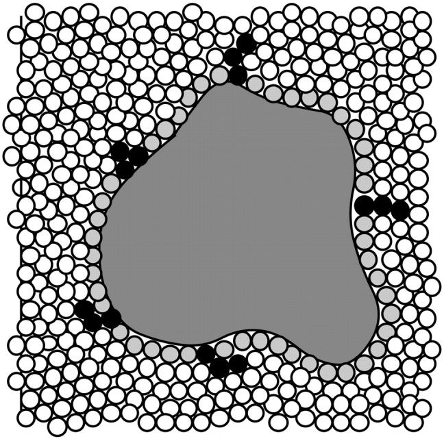
Representation of a solvated protein. The small circles represent water molecules. Cross-hatched circles depict the solvation layer in contact with the protein. The black triple circles represent modes of contact of cosolvent molecules interacting with the protein by replacing a contact water molecule. Cosolvents making double contacts with the protein, like the one at 10 o'clock in the diagram, are not specifically considered in the model.
The “accessible surface area” (ASA) can be computed for any known structure using the methods of Lee and Richards (1971) or Connolly (1983). For water, a probe radius of 1.5 Å is assumed. This is intermediate between recently proposed values for polar and nonpolar contacts (Li and Nussinov, 1998). A mean area of 10 Å2 is assumed for each water molecule. This value has been used by previous workers (Chothia, 1975; Schellman, 1978; Colonna-Cesan and Sander, 1990). The number of sites and therefore the number of first layer water molecules can then be calculated from the total area.
The present study differs from previous ones in a number of ways, which will now be outlined:
Inclusion of excluded volume in the calculations. In previous reports from this laboratory, excluded volume effects were neglected. It was thought that utilizing molalities, which are detached from the measurement of volume, would largely compensate the excluded volume effect. In addition, for protein unfolding we are considering a difference in excluded volume between two states of the same molecule so that there should be considerable cancellation. As will be seen by direct calculation in a later section, there is compensation and cancellation, but the excluded volume effect is nevertheless quite large as has been noted by other authors (Wills et al., 1993; Colonna-Cesan and Sander, 1990; Saunders et al., 2000; Ebel et al., 2000). We emphasize that we are discussing the excluded volume of a large molecule for a small molecule and not the large molecule-large molecule exclusion that has been emphasized in many recent papers (Minton, 1998; Wills et al., 2000).
-
Volume fraction, ϕ, will be used for equilibrium calculations rather than mole fraction or molality. The probability of a molecule being at a point near the surface of a protein is proportional to its concentration. If the molecule contains more than one group, e.g., NH2, OH, C=O, there are a number of ways that it can penetrate the solvation shell. For urea it would be three, not counting bifurcated or flat contact. The concentration should then be multiplied by a factor that provides a weighted mean over possible contact modes. Use of volume fraction at least approximates the use of such a factor. For example, the ratio of the volume of a urea molecule to a water molecule is 2.5. This gives a more realistic description of the probability of contact.
Another substantial advantage is that volume fractions and molar concentrations are easily interconvertible, making comparison with experimental papers easier. Volume fractions are calculated from molarities via the formulas Subscripts 1, 2, and 3 refer to water, protein, and cosolvent, respectively. C indicates molarity. Protein concentration will be considered to be sufficiently small that
  is negligible in comparison to the other components.
  values of solvent species will be assigned their low concentration values and considered as constants. Equilibrium at a site follows the solvent exchange relation
where
(1)  and
and  represent the occupation of the site by solvent or cosolvent, respectively. The subscripts will be used to indicate a single contact site for interaction with a solvent or cosolvent molecule. These relations are formally the same as in a previous discussion where mole fractions rather than volume fractions were used (Schellman, 1987).
 Activity coefficients are ignored. Even though accurate values of activity coefficients are available for most denaturants and some osmolytes, there are reasons for neglecting them. One reason is pragmatic. Osmolytes and especially denaturants are far from ideal in aqueous solution. On the other hand, it is known that the effects of these and other reagents on other solutes tend to be linear in concentration (Pace plot for unfolding of proteins (Greene and Pace, 1974)), Sechinov's equation (Harned and Owen, 1950, Eq. 12-10-3). Concentration-dependent activity coefficients lead to deviations from Eq. 2 (below) unless they cancel. This nonlinearity was extensively observed in a previous publication that made use of activity coefficients (Schellman, 1990).
In addition, inspection of the way in which activity coefficients are normally introduced into equilibria like Eq. 1 reveals an inconsistency. The argument is clearer in terms of molarity, and since molarity and volume fraction are essentially in direct proportion to one another, the results will apply to volume fractions as well. On a molarity scale for a nonideal solution, Eq. 1 would be written as
 |
where C1 and C3 are the molarities of the principal solvent and cosolvent, y1 and y3 are the activity coefficients of the two solvent components, and  and
and  are the same as in Eq. 1. Activity coefficients are inserted for the bulk solution components because we know how to do it, but not for the bound components. It does not seem possible to design experiments that would measure a thermodynamic activity coefficient for loosely bound ligands on a protein surface.
The activity coefficient of, say, a urea molecule in solution results from its interaction with other urea molecules. By ignoring activity coefficients for bound molecules, we assume that the interactions of a urea molecule in contact with a protein molecule do not differ very much from those of a free urea molecule. This is illustrated in Fig. 1, which shows that a molecule bound by a single contact to a protein is still largely surrounded by solvent. The assumption of solution interactions for the free molecule, but not for one in contact with the protein, is likely to increase errors rather than eliminate them.
With these matters out of the way, we may proceed to an overall description of the method. The standard formula for unfolding in the presence of a cosolvent is (Greene and Pace, 1974)
 |
(2a) |
which can also be expressed in terms of equilibrium constants
 |
(2b) |
where m or  are measures of the change in
  or
or  caused by the addition of the cosolvent. In most work this interaction term has been equated to the free energy of contact of component 3 with sites on the protein molecule. In the present context it consists of two parts, the contact free energy and the excluded volume free energy. Later it will be seen that these parts are additive:
 |
(3) |
We drop the unf subscript at this point.  is the free energy associated with excluded volume. Its evaluation will be discussed in Section 4, “Calculation Strategy”. The contact free energy,
  is known to be related to the binding polynomial emphasized by Wyman (Schellman, 1975). Because of the analogy between mole fractions and volume fractions, we replace the mole fractions in Eq. 19 of Schellman (1987) by volume fractions to obtain the interaction at a specific site, s,
 |
(4) |
with Ks defined in Eq. 1. In the limit of very small protein concentration,  and
and
 |
(5) |
The −1 factor subtracts the probability that 3 occupies a site in a random fashion determined by the composition of the solution. Note that if Ks = 1, the ratio of (3) molecules to (1) molecules on the site becomes equal to the ratio of the volume fractions in the bulk solvent. In this case there is no preferential solvation and  Converting to concentration,
 |
(5a) |
We introduce the constant  because it turns out to be directly related to the quantity determined by experiment.
We also know that empirically the free energy is a linear function of concentration (Myers et al., 1995). Expanding the log in Eq. 5 to the linear term
 |
(6) |
the total interaction is given by a summation over all sites:
 |
(7) |
In the last expression, we replace the sum over all exposed sites by the number of sites multiplied by the average K′ per site. In Section 6, “Results”, it will be seen that the assumed linearity is in agreement with numerical results but leads to a small error.
Note that the sites are expected to be very heterogeneous. A guanidinium ion, for example, will be attracted to negative charges and H-bond acceptors, repelled by positive charges and proton donors, and will have a variety of interactions with other polar and nonpolar interactions. Also Ks remains an equilibrium constant based on volume fractions even though we have transformed the results to molarity to match experimental results.  and
and  are not true equilibrium constants. This is demonstrated by the fact that they can have a negative sign.
FORMULA FOR DATA ANALYSIS
As we shall see, there are two factors that determine the interaction of solvents with sites on a protein. The first is solvation preferences at the site, and the second is excluded volume. These concepts will be developed in terms of a simple model of interaction in gases. This is an allowable approach since the McMillan-Mayer theory shows that the interaction of a pair of molecules in a gas can be treated in exact analogy with the interaction of a pair of molecules in a principal solvent (e.g., water), which does not make a direct appearance in the formulation (Hill, 1960). For the pressure, which is the osmotic pressure for a solution, we make use of the virial equation
 |
(8) |
where the Bij are virial coefficients associated with the interaction of a molecule of type i with a molecule of type j. See Appendix for more details. B23 is the term we are interested in since it evaluates the principal interaction between component 2 and component 3. Suppose molecules of type 2 and 3 are hard spheres of radii ra and rb, so that they cannot approach one another any closer than the distance ra + rb. For this case, the molecular excluded volume is  and the virial coefficient, B23, equals the molar excluded volume, X = Nav, where Na is Avogadro's number.
This is shown in all elementary texts of statistical mechanics and in Tanford's book (Tanford, 1961, page 192). The symbol X will be used for the excluded volume to distinguish it from real molar volumes. Excluded volume decreases the free volume for the molecules and increases the pressure.
The second example is a weak interaction between components A = 2 and B = 3 governed by the equilibrium
 |
where α is CAB. For small concentrations it is readily shown that α = KCACB. Summing the contribution of all three species to the pressure
 |
(9) |
Putting  and comparing Eqs. 8 and 9, we see that for this case
  . Association lowers the number of molecules in the system and decreases the pressure.
We concentrate on the B23 term, which deals with the interaction of protein with cosolvent. The two models reflect the current practice in the discussion of protein solvent interactions. Some authors assume that excluded volume is the major contributing factor, especially for osmolytes; others assume the dominance of selective interaction, especially for denaturation. For the general case, we make the heuristic assumption that B23 is simply the sum of the association and excluded volume terms, i.e.,
 |
See the Appendix for a discussion that demonstrates this additivity. For the thermodynamics of unfolding, the interaction term must be summed over all sites. In addition, we want the difference in B23 between the folded and unfolded states, i.e.,  Introducing these changes,
 |
(10) |
ΔX is the difference in excluded volume, unfolded minus folded, and the sum is over all sites exposed by the unfolding.  is the apparent equilibrium constant for site s introduced in Section 2, “Physical Aspects of the Model”. This expression is especially clear in the molecular discussion of the appendix.
Measurements of osmotic pressure are not a practical way to study the interactions of solvent with proteins, but  has simple relationships with quantities that are measured. These are the excess free energy change caused by the denaturant or osmolyte (
 or m values) and the preferential interaction coefficient. This paper will concentrate on the former. Using thermodynamic arguments it is possible to show that
 |
(11) |
This is the relation that connects denaturation studies with the change in virial coefficient. This will be proved in a later, more technical, article. Combining Eqs. 10 and 11,
 |
(12) |
This is the operative formula for the calculation that evaluates the solvation term. Rather than trying to predict the values of m or  the experimental values of m and calculations of the excluded volume are used to obtain values for the selective interaction with solvent.
CALCULATION STRATEGY
The present approach is analytical.  is known from experimental m or
  values. As discussed below, good estimates of
  the change in excluded volume, can be made from the structure of the native protein and a reasonable model for the unfolded protein. What we don't know about these systems is the interaction term,
  , and the aim of the procedure is to evaluate this quantity from the experimental data and volume calculations via Eq. 12. This result is then converted into an average interaction per site exposed during denaturation. This strategy was also adopted by Saunders et al. (2000) but with a different model and type of calculation. Because of the excluded volume contribution, this term has been consistently underestimated in most publications, including the author's.
Excluded volumes and accessible surface areas were computed using the Connolly MSRoll program (Connolly, 1993). Atomic structures are used for the native and denatured protein. The small molecule cosolvents are represented as spheres. The effective radii of these spheres are obtained from their molecular coordinates determined by x-ray diffraction. Each atomic position (or group like-CH3) of a cosolvent molecule is surrounded by a sphere with a radius equal to its van der Waals radius (McCammon et al., 1979). Three principal diameters of the cosolvent molecule are calculated, averaged, and divided by two to obtain a mean radius (see Table 1). The accessible surface area (ASA) is the surface that goes through the centers of all the solvent spheres in contact with the protein (see Fig. 1). This area, calculated for both the folded and unfolded molecule in contact with water, is taken as the solvent contact area. Water is assumed to occupy an area of 10 square Å (Chothia, 1975; Schellman, 1978; Colonna-Cesan and Sander, 1990) so that the number of contact sites is obtained from the accessible surface area by dividing by 10.
TABLE 1.
Ratios of probe volumes to default area, X(rp)/ASA(1.5 Å)
| No. | Protein | rp = 1.5 | rp = 1.8 | rp = 2.2 | rp = 2.4 | rp = 2.96 | rp = 4.0 |
|---|---|---|---|---|---|---|---|
| 1 | RNT | 1.903 | 2.215 | 2.651 | 2.887 | 3.586 | 5.043 |
| 2 | RN | 1.900 | 2.212 | 2.648 | 2.883 | 3.582 | 5.036 |
| 3 | LZ | 1.894 | 2.206 | 2.643 | 2.878 | 3.576 | 5.024 |
| 4 | SN | 1.890 | 2.201 | 2.639 | 2.874 | 3.572 | 5.027 |
| 5 | T4L | 1.896 | 2.208 | 2.644 | 2.879 | 3.576 | 5.025 |
| Av. | 1.896 | 2.208 | 2.645 | 2.880 | 3.579 | 5.031 | |
| SD | 0.005 | 0.005 | 0.005 | 0.005 | 0.005 | 0.008 |
The excluded volume is different for each cosolvent. To calculate the volume within the ASA, rather than the molecular surface area, the probe radius is set to zero and the van der Waals radii of the protein atoms are increased by the radius of the probe molecule. I thank J. W. Ponder and M. L. Connolly for suggesting this strategy.
The determination of the surface areas and excluded volumes of the native proteins is straightforward. The Connolly program MSRoll accomplishes both calculations using the crystal structure coordinates (Connolly, 1993). Five well-studied proteins were selected for analysis: ribonuclease-T (RNT), ribonuclease-A (RN), hen egg white (HEW) lysozyme (LZ), staphylococcus nuclease (SN), and T4 lysozyme (T4L). The protein database indices for the structures are shown in Table 2.
TABLE 2.
Experimental data
| Protein | PDB No. | m | Δb23 | Cm | pH, T | Ref. |
|---|---|---|---|---|---|---|
| A Experimental parameters for urea unfolding | ||||||
| RNT | 9RNT | 1.21 | −2.03 | 5.3 | 7.0, 298 | * |
| RN | 1RND | 1.14 | −1.91 | 6.5 | 7.0, 298 | † |
| LZ | 1LKS | 1.29 | −2.16 | 6.8 | 7.0, 298 | † |
| SN | 1SNO | 2.38 | −3.99 | 2.56 | 7.0, 296 | ‡ |
| T4L | 2LZM | 2.00 | −3.36 | 6.3 | 7.0, 295 | § |
| B Parameters for unfolding in guanidinium chloride | ||||||
| RNT | 9RNT | 2.56 | −4.30 | 2.99 | 7.0, 298 | ¶ |
| RN | 1RND | 3.09 | −4.97 | 2.99 | 7.0, 298 | ¶ |
| LZ | 1LKS | 2.33 | −3.91 | 4.24 | 7.6, 298 | ‖ |
| SN | 1SNO | 6.83 | −11.5 | 0.81 | 7.0, 293 | ‡ |
| T4L | 2LZM | 5.50 | −9.38 | 2.20 | 7.4, 295 | § |
| C Parameters for folding in TMAO (unfolding data from Baskakov and Bolen (1998)) | ||||||
| RNT | 9RNT | −1.77 | 2.97 | 1.26 | 7.0, 298 | – |
| SN | 1SNO | −2.55 | 4.28 | 1.57 | 8.8, 303 | – |
The surface area and excluded volumes of the unfolded form pose a problem for which there is at present no definitive answer. It is easy to obtain a surface area for the polypeptide chain in an extended conformation, and results have been available for many years (Chothia, 1975). The problem is that there are intramolecular contacts in the unfolded state and the fraction of surface area (and excluded volume) that is obscured in this way probably varies from protein to protein and definitely depends on the solvent medium. Many years ago, Tanford's group studied the extent of unfolding of proteins in urea and guanidinium chloride, concluding that complete unfolding occurs only at high concentrations of the latter and is not reached in the former even at high concentration (Aune et al., 1967; Tanford et al., 1966). Bolen's group has shown that the osmolyte Trimethylamine-N-oxide (TMAO) has the opposite effect to guanidinium chloride in that it leads to a smaller size distribution of the unfolded protein as its concentration is increased (Qu et al., 1998). Standard polymer theory interprets this as resulting from increased intramolecular contact and therefore diminished surface area and excluded volume. Shortle has found that the unfolded states of staphylococcus nuclease and its mutants are not completely unfolded and have a variable residual structure depending on mutations (Shortle and Meeker, 1986; Shortle et al., 1992).
Creamer et al. (1997) have taken up this problem. They selected 43 peptide chains that occur in unordered regions of globular proteins. The ASA of these chains was calculated retaining the conformations found in the crystal structures. This was considered to be a lower limit for the surface area, because these chains would be expected to have more frequent intramolecular contacts and therefore lower surface area than freely varying peptide chains in solution. They obtain an upper limit for the ASA of an unfolded chain by converting these chains to a relaxed extended conformation with essentially no intramolecular contacts and determining the accessible surface area for the chains in the sample. Their reasonable assumption is that a real unfolded chain will have fewer intramolecular contacts than a chain that is part of a globular protein and more than an extended chain. As a consequence, the ASA of a real unfolded chain should be intermediate between these two limits. They provide tables so that an ASA can be calculated for both limits from the amino acid composition. Their results will be used in the calculations below. Because of the uncertainty and variability of the mean structure of the unfolded form, there is no firm ground for selecting a best value for a real protein under given solvent conditions. What can be done is to examine the two limits for each system and to take the average of the two extremes as a representative value. The excluded volume effect is large and any reasonable estimate is better than ignoring it.
The excluded volumes of the unfolded chains create a special problem, which is discussed in Section 5, “Excluded Volume and Accessible Area”.
The procedure
Evaluate the ASA of the native protein (ASAnative) using the Protein Data Bank coordinates with a probe radius representative of a water molecule (here, 1.5 Å).
Evaluate the ASA for water molecules (ASAunf) of the unfolded protein at both limits, and take the mean value as an approximation to the correct ASA for the unfolded protein.
Subtract ASAnative obtained in (1) from ASAunf obtained in (2) to get ΔASA for the unfolding. Divide by 10 for the change in number of contact sites for water molecules that occurs with unfolding.
Evaluate the excluded volume (Xnative) of the native protein using a probe radius for the osmolyte or denaturant under consideration. This is done by setting the probe radius equal to zero and adding the cosolvent radius to the van der Waals radii of the atoms of the protein.
Evaluate the excluded volume of the unfolded chain for the osmolyte under consideration. Our indirect method of doing this is explained in Section 5, “Excluded Volume and Accessible Area”.
Subtract Xnative obtained in (4) from Xunf obtained in Section 5 to get ΔX for the cosolvent arising from the unfolding.
Obtain values of Δb23 or m from the literature and evaluate
 via Eq. 12.
The partial molar volume of cosolvent,
 is usually available from the literature or from density data. In this paper, it is assumed to be a constant for simplicity. We can then calculate the site average
  from the definition in Eq. 6.
The mean site occupancy by cosolvent can then be obtained via the relation
 and compared with the random occupancy,
  In this paper,
  is evaluated at the transition concentration, so
  and
and 
EXCLUDED VOLUME AND ACCESSIBLE AREA
The excluded volume for a probe molecule is the sum of the real volume of the target molecule estimated from van der Waals radii plus a gap space or envelope, around the molecular surface, where the center of the probe molecule cannot penetrate. Excluded volume = target volume + gap volume (see Fig. 2). The thickness of this gap layer is the van der Waals radius of the probe molecule. The gap volume increases with surface area. For a planar surface, it is given by the area times the probe radius, A × rp, where r is the radius of the probe sphere. In a recent paper, the gap volume was estimated by multiplying the surface area by the probe radius (Ebel et al., 2000). For a sphere, it is approximately A × rp (1 + rp/Rt); for the curved surface of a cylinder, it is A × rp (1 + rp/2Rt). Rt is the radius of the target sphere, and it is significant that 1/Rt is its curvature. These systems exemplify the general relation of Isihara, which gives the gap volume as the surface area times an averaged curvature over the surface (Isihara and Hayashida, 1951a,b).
FIGURE 2.

The nature of excluded volume. The center of the small probe sphere is restricted from a volume that is the sum of the volume of the large sphere plus the gap volume indicated in the drawing. The larger outer sphere is the accessible surface area for the smaller probe. The volume within the ASA is the excluded volume.
In proteins, the types of atoms and the curvature of their surfaces are usually strongly limited (C, O, N, S, (H)) and their elemental compositions are very similar. Space-filling models of molecules consist of overlapping spheres of the van der Waals radii of these atoms. With the mean curvature very similar for most protein surfaces, we would expect a proportionality between the gap volume and the accessible surface area that increases with probe radius as in the above formula for spheres. We tested this by examining the ratio rp /ASA(1.5) for our set of five proteins. GapVol is defined as X − protein molecular volume, the latter quantity being also a standard output of the MSRoll program. GapVol was calculated for the five extended proteins using the probe radius, rp, for the six solvent species: H2O, Cl−, urea, guanidinium, TMAO, and sucrose. Proportionality was observed. For a 1.5 Å probe, the standard deviation for (gapVol/ASA was ∼1 part in 1500. The standard deviation increased very slowly as rp was increased. Of more interest to this investigation is the fact that the ratio of the excluded volume for a probe of radius rp, i.e., X(rp)/ASA(1.5) is also essentially constant for extended chains (see Table 1). This table permits us in principle to go directly from surface areas to excluded volumes for the various probes. Our use of this idea was to apply it to the estimated areas of unfolded chains of Creamer et al. (1997) to convert these areas into estimated excluded volumes:
 |
The constant depends upon rp but not on protein. There should be no problem with the extended chain. The ASA and excluded volumes of extended chains are simply the sums of independent contributions of the amino acids, a procedure initiated by Chothia (1975). There is no structural component, only the peptide chain with almost independent side chains. Even for the amino acids themselves, the standard error in excluded volume divided by surface area is in the neighborhood of 1%. The small differences among various amino acids are diminished further by averaging over the rather similar compositions of globular proteins.
Applying the results to unfolded chains that are not extended is more questionable. These chains have partial elements of structure that lead to intramolecular contacts or near contacts that diminish the surface area. This is obvious from the results of Creamer et al. From the above analysis, it is clear that the excluded volume will also be reduced because of these contacts. This should cancel errors appreciably. Adopting the method of Creamer et al. by analyzing 43 peptide chains with six probes would be a major project that would delay the present publication considerably. This would be a useful study of the effect of intramolecular contacts on the unfolded chain. On the other hand, it would only help the present problem in an approximate way. As discussed above, it is not yet possible to quantify the surface area of an unfolded peptide chain under varying solvent conditions. All we can do is make a reasonable estimate. Our provisional approach is to take the average of the excluded volumes, calculated via the proportionality constants of Table 1, for the extended chain and for the lower bound estimate of Creamer et al. We have also examined the limits by making use of the low and high limits of the surface area.
RESULTS
The procedure for calculation has been outlined in previous sections, so the results may be presented in tabular form. Table 2, A–C, contains data on the unfolding of the selected five proteins. The choice of references therein was partially guided by an extensive review of such studies (Myers et al., 1995). The m and Cm values were taken from the original papers. Contact interactions with a protein are dependent on pH and temperature, but apparently only the pH dependence has been studied (Pace et al., 1990). We have tried to select data for which the pH varies as little as possible. Measurement of the temperature variation would be of great importance since it would lead to values for the enthalpy of solvation by the cosolvent. m values are converted to  (Eq. 11), since all the theoretical quantities have the units of L/mole = (molarity)−1.
Partial molar volumes for the cosolvents and mean radii of the cosolvent molecules are listed in Table 3. The mean radii were obtained from crystal coordinates of the cosolvent molecules adding a van der Waals radius for each atom or group like CH3-. A standard set of van der Waals radii (McCammon et al., 1979) was used, the same as in Connolly's MSRoll program. The  entries were obtained from density data on water-cosolvent mixtures using the methods outlined in a previous publication (Schellman and Gassner, 1996). For the purposes of this paper,
  was assumed to be a constant and the small variations with concentration were ignored. The value for the guanidinium ion was found by subtracting the partial molar volume of the chloride ion, estimated by Mukerjee (1966), from that of guanidinium chloride.
TABLE 3.
Cosolvent properties
| Cosolvent |
 (L/mole)* (L/mole)*
|
Ref. | rp(Å) | Ref. |
|---|---|---|---|---|
| Urea | 0.046 | † | 2.2 | ‡ |
| TMAO | 0.073 | § | 2.95 | ¶ |
| Gdn.HCI | 0.072 | † | ||
| Cl− | 0.022 | ‖ | 1.81 | ‖ |
| Gdm+ | 0.050 | 2.4 | ** | |
| Sucrose | 0.211 | †† | 4.3 | ‡‡ |
 assumed constant.
Volumetric data from Kawahara and Tanford (1966).
Mean of three principal radii. Coordinates from National Institute of Standards and Technology Chemweb: www.nist.gov/srd/online.htm.
Volumetric data from Lin and Timasheff (1994).
Calculated from crystal data of Mak (1988).
Estimated by Mukerjee (1961).
Calculated from data of Averbuch-Pouchot and Durif (1993).
Calculated from data in CRC (1965), page D163.
Calculated from dimensions of Garrod and Herrington (1970).
Note that the Δb values for TMAO are positive, an indication that the unfolded form is destabilized relative to the folded form and the transition is inverted.
All the empirical quantities required for the calculation are listed in Tables 2 and 3. The procedure has been completely outlined in previous sections so we may go immediately to the results that are shown in Table 4, A–C, for urea, guanidinium chloride, and TMAO.
TABLE 4.
Results
| Protein | Xunf | Xnat | ΔX | ΔB | ΣK′ |  |
Kav | Occupation | Random |
|---|---|---|---|---|---|---|---|---|---|
| A Results for urea unfolding | |||||||||
| RNT | 19.0 | 14.3 | 4.67 | −2.03 | 6.70 | 0.0102 | 1.224 | 0.283 | 0.244 |
| RN | 24.2 | 17.5 | 6.66 | −1.91 | 8.57 | 0.0101 | 1.221 | 0.342 | 0.299 |
| LZ | 25.3 | 18.1 | 7.24 | −2.16 | 9.40 | 0.0100 | 1.227 | 0.358 | 0.313 |
| SN | 30.8 | 20.5 | 10.3 | −3.99 | 14.3 | 0.0123 | 1.269 | 0.145 | 0.118 |
| T4L | 33.7 | 23.9 | 9.84 | −3.36 | 13.2 | 0.0104 | 1.229 | 0.334 | 0.290 |
| Protein | Xunf | Xnat | ΔX | ΔB | ΣK′ |  |
Occupation by Gdn+ | Random, ϕ+ | |
|---|---|---|---|---|---|---|---|---|---|
| B Results for guanidinium chloride unfolding | |||||||||
| RNT | 36.6 | 28.0 | 8.6 | −4.30 | 12.8 | 1.40 | 0.194 | 0.147 | |
| RN | 46.4 | 34.3 | 12.1 | −4.97 | 7.1 | 1.41 | 0.195 | 0.147 | |
| LZ | 48.6 | 35.3 | 13.3 | −3.91 | 17.2 | 1.34 | 0.260 | 0.208 | |
| SN | 59.2 | 42.2 | 17.0 | −11.5 | 28.5 | 1.50 | 0.058 | 0.040 | |
| T4L | 64.8 | 46.7 | 18.1 | −9.38 | 27.5 | 1.41 | 0.146 | 0.108 | |
| Protein | Xunf | Xnat | ΔX | ΔB | ΣK′ |  |
Kav | Occupation | Random occupation |
|---|---|---|---|---|---|---|---|---|---|
| C Results for folding in TMAO* | |||||||||
| RNT | 25.7 | 16.9 | 8.8 | 2.97 | 5.84 | 0.0089 | 1.12 | 0.102 | 0.0920 |
| SN | 41.6 | 24.1 | 17.5 | 4.28 | 13.2 | 0.0114 | 1.16 | 0.131 | 0.1146 |
The units of Xunf, Xnat, ΔX, ΔB, and ΣK′ are L/M.
Distributions in the last two columns are evaluated at Cm, which varies for different proteins. See Table 2 B.
Urea
Looking at the gross properties of the interaction revealed in Table 4 A (columns 4–6), we see that in each case there is a large change in excluded volume, ΔX, which can be larger than the molar volume. The latter can be estimated (in liters per mole) by multiplying the molecular weight by 0.7/1000 (Quillan and Matthews, 2000). ΔX stabilizes the folded form. But the interaction term,  which contributes negatively to ΔB, is even larger, leading to a net negative ΔB. This result is depicted in Fig. 3 for all five proteins. Urea is a denaturant because its contact interactions with the exposed interior of an unfolded protein are attractive and large enough to overcome the ΔX term. Excluded volume stabilization is a common element in all cosolvent-protein interactions and it is invariably positive for unfolding (increased surface area). Note that ΔX, ΔB, and
  are all global properties, roughly proportional to exposed surface area, and therefore generally increase with molecular weight. SN provides an exception.
FIGURE 3.


The balance of forces involved in stabilization or destabilization (see Eq. 10). The stability of the folded form is proportional to ΔB, which is directly related to m values. Negative ΔB is a measure of instability. ΔB is the balance of two thermodynamic forces: the change in excluded volume and the change in interaction with the cosolvent are represented by ΔX and  , respectively. For unfolding, ΔX is always positive. For denaturants, the interaction is sufficiently strong that the stabilizing effect of the excluded volume is overbalanced, leading to a negative ΔB. A–C are bar diagrams for urea, guanidinium, and TMAO, respectively.
Column 7 of Table 4 A contains the values for  obtained via Eq. 12. We can now justify the representation of
  by
by  which leads to the linear Pace plot. Ribonuclease and urea will be used as an example, since Cm has a high value, and should provide a relatively stringent test. Plots of
  and
and  are presented in Fig. 4 using the value of
  from Table 4 A. The plots range over four units of molarity centered on the ribonuclease Cm of 6.5 M. In an experiment, the
  plot would certainly be taken as linear even with very small experimental errors. A linear least-square analysis of this curve yields an intercept of 0.002 and a slope of 0.0095, which are to be compared to the correct values of zero and 0.0101. The agreement with the intercept indicates that the extrapolation to zero concentration should give the correct value of
  This is support for the most widespread use of these plots. On the other hand, the apparent slope is ∼6% lower than that of an exact straight line. In a linear analysis of data,
  and
and  would be underestimated by the same percentage. At the present time, this type of error must be accepted since experimentally the only information available is the approximate straight line.
FIGURE 4.

Demonstration that  is essentially linear in x.
  Values of
  and Cm were taken from data for the denaturation of ribonuclease A in urea. See text.
The last three columns of Table 4 A are concerned with the average interactions at the sites. The equilibrium constants are the average site equilibrium constants, Kav, defined by Eq. 1 on a volume fraction basis and obtained via Eq. 12. The value for staphylococcus nuclease, SN, is significantly higher than the other four proteins, which differ by less than 0.005 from a mean of 1.225. The unfolding anomalies of SN are well known (Shortle and Meeker, 1986) and will be seen in most of our results. The close agreement for the four other proteins is consistent with a free energy that is proportional to the number of sites, presumably arising from a similarity in the composition of the areas exposed by unfolding. This is different from the usual free energy versus area comparison because of the inclusion of excluded volume. However, excluded volume is also proportional to area as was shown in Section 5, “Excluded Volume and Accessible Area”. Both  and
and  are measures of the strength of the contact interaction, the former for the entire protein, the latter for the average site. Later these quantities will permit a comparison of the interactions of urea, guanidinium and TMAO.
An overall understanding of the results in Fig. 3 and Table 4 requires a distinction between preferential interaction, a thermodynamic quantity accessible to direct measurement, and preferential solvation, which is defined as the excess or deficit of a component in the solvation shell around the protein molecule relative to its bulk concentration. (The dual use of the term preferential interaction as a thermodynamic measurement and as preferential solvation is so engrained in the author's mind that misuse has been hard to eliminate. To protect the reader from the same error, the words solvation and interaction are italicized throughout the rest of this paper to emphasize the difference between these quantities.) If an excess of component 3 tends to accumulate in the neighborhood of a protein relative to its macroscopic concentration, the preferential solvation is positive for component 3 and negative for component 1, and vice versa. Table 4 A and Fig. 3 A illustrate the positive preferential solvation for urea. The random occupation of a site by components 3 or 1 is simply given by their volume fractions in the solution (last column of Table 4 A). The actual site occupation may be calculated by the usual binding polynomial formula,  given in the next to last column. Urea preferentially solvates the exposed areas of all the proteins. This interpretation of the mechanism of solvent denaturation goes all the way back to Wu (1931).
From the last two columns of the table, it is seen that there is an excess of only ∼15% in the occupation (23% for SN) as a result of the interaction; 85% of the occupation is a random event. Although all interactions contribute to the unfolding, the selectivity (preferential solvation) is only 15%. This aspect of the problem will be discussed in a later paper. It is also recognized in the models of Timasheff and Record, who discuss binding as an excess over bulk concentrations in the neighborhood of the surface (Lee and Timasheff, 1974; Record and Anderson, 1995; Courtenay et al., 2000).
Preferential interaction, on the other hand, includes all factors that increase or reduce the quantity of component 3 in the solution when the concentration of the protein is increased. It was shown by Hill (1957) and especially pertinently by Wills and Winzor (1993) that preferential interaction is proportional to the virial coefficient between components 2 and 3 and therefore contains an excluded volume term. Solvent denaturation has long been considered as primarily due to preferential solvation. Several investigators have suggested that stabilization by osmolytes results from the excluded volume effect alone. It is only very recently that both terms in Eq. 10 have been recognized as factors in stabilization studies (Saunders et al., 2000; Davis-Searles et al., 2001). The present paper presents a model that applies to denaturation and stabilization and gives realistic results for the preferential solvation term.
Ignoring nonideality corrections, the change in preferential interaction (associated with unfolding is given by  (Casassa and Eisenberg, 1964); i.e., it is proportional to the length of the third bar associated with each protein of Fig. 3 A. On the other hand, preferential solvation is given by
  i.e., it is represented by the length of the central bar in the figures. As will be seen below, it is possible for the preferential solvation and the preferential interaction to be opposite in sign. The excluded volume term can partially cancel or even override the preferential solvation term.
TMAO
The results for TMAO are shown in Table 4 C and Fig. 3 C. There are only two entries in the table because the folding effect of TMAO has only been observed reversibly for ribonuclease-T (RNT) and staphylococcus nuclease (SN) (Baskakov and Bolen, 1998). Both proteins were altered to destabilize the native form. RNT was carboxamidated and SN was subjected to a strongly destabilizing mutation. The calculations of ΔX were performed for the native proteins, ignoring small changes in the surface area and volume that result from the alteration of the proteins. To make a consistent comparison with denaturants, we continue to consider the free energy of unfolding. Since the proteins fold with increasing TMAO, the result is a negative m and a positive Δb and ΔB. This was pointed out in the original experimental paper. The relation  still holds. Since both ΔB and ΔX are positive, there are two possibilities: 1), Kav is <1 so that
  is positive; both terms contribute to the stabilization. 2), Kav is >1; on average the interaction is favorable but not enough to overcome the positive ΔX. The results in Table 4 C show that the second possibility is the correct one. The excluded volume contributions are larger than for urea because TMAO is a larger molecule. Compare the probe radii in Table 3.
Comparing  in Table 4, A and C, we note that the intrinsic interaction of exposed surface groups with TMAO is favorable on the average but is diminished by a factor of one-half. We thus have the same general picture for TMAO as for urea. There is a generic excluded volume effect that will tend to stabilize the folded form. Opposing this are the contact interactions at the exposed surface that on the average are favorable and tend to destabilize the folded form. Only the relative size of the two effects differentiates between the two types of reagent. TMAO stabilizes proteins because its excluded volume is larger and its interaction with solvent smaller than that of urea.
Fig. 3 C and Table 4 C show that the contact free energy of exposed surfaces is mildly negative for TMAO. This leads to local preferential solvation with the osmolyte rather than local preferential hydration. These statements are not in disagreement with the findings of Timasheff's group that osmolytes are preferentially hydrated. Preferential interaction measurements are thermodynamic and are proportional to Δb, i.e., the algebraic sum of the excluded volume and the contact interaction term. (Preferential interaction studies are usually measured in mass or molality units and are therefore proportional to Scatchard's Δβ rather than Δb. It may be shown that the use of molality corrects for molecular volumes, but not for excluded volumes.) In the present analysis, preferential hydration occurs in osmolyte solutions because of the dominance of the excluded volume term.
Wang and Bolen (1997) studied the transfer free energies of amino acids from water to TMAO solutions and analyzed their results in terms of backbone and side chain transfers. Significantly, the free energy of transfer of peptide groups changes from the negative value it has for denaturants such as urea to positive values for TMAO. They conclude that this preferential solvation by water of peptide groups is the dominant cause of the stabilization of proteins by TMAO.
There are some difficulties in making comparisons between the free energy of transfer method and the present model in which the free energy is decomposed into excluded volume and preferential solvation, because this decomposition is not made in experimental transfer studies. A partial harmonization of the two sets of results is as follows: Courtenay et al. (2001) have observed that peptide backbone makes up ∼13% of the area exposed by the unfolding of a typical globular protein. They also make the point that the interaction of peptide groups with urea is ∼4 times as strong as the typical exposed area of a protein as measured by m values of equivalent areas. We have found that the average preferential solvation by TMAO, measured by  is only half that of urea and this is most certainly attributable to the cosolvent rejection by peptide groups observed by Wang and Bolen. With the present analysis, there are two effects of TMAO that lead to the stabilization of the folded form. One is the excluded volume and the other is the reduced affinity of proteins for a TMAO solution as depicted in Fig. 3 C. This combination prevents the preferential solvation from overriding the excluded volume term as it does with denaturants. Viewed in this way, there is no qualitative disagreement between the two interpretations. A more meaningful comparison will require a detailed study of the free energy of transfer method that includes excluded volume effects.
If  were negative for TMAO, we would have the conditions for a Flory-Fox collapse and aggregation of the protein. It has in fact been shown that proteins contract in size and tend to precipitate at higher TMAO concentrations (Qu et al., 1998). This was interpreted as enhanced intrachain interactions resulting from the positive contact free energy of peptide groups with TMAO, which is quite reasonable and in accord with polymer theory. On the other hand, it could be expected that at least a small affinity for a solute, i.e.,
  is required to form a stable solution. This presumably results from the nonpeptide groups of the protein.
Guanidinium chloride
For an ionic substance, a small change in formulation is necessary. The relation that replaces (ϕ1 + Ksϕ3) in Eq. 4 is
 |
(13) |
where  and
and  are the site binding constant (volume fraction basis) and volume fraction of the cation, and
  and
and  apply to the anion. This relation is obtained in the same way as Eq. 5. See Schellman (1987) for a similar discussion involving mole fractions rather than volume fractions. It is not possible to evaluate
  or
or  individually by purely thermodynamic means, though comparison with other anions or cations often will establish relative magnitudes. Empirically it is clear that the dominant denaturant effect in this case comes from the guanidinium ion, Gdm+, though it would be a mistake to consider the chloride as negligible. See Wong and von Hippel for a demonstration of anion effects and Baldwin for a further discussion (von Hippel and Wong, 1964; von Hippel and Wong, 1965; Baldwin, 1996). With no clear-cut directive, we will arbitrarily assign all the interaction to the guanidinium ion by putting
  for the anion. If relative values for Gdm+ and Cl− become available, the calculations can be redone. With this substitution we have
 |
(14) |
The populations at a given site will then be  and
and  for water, guanidinium ion, and chloride ion, respectively.
The results are shown in Table 4 B and Fig. 3 B. Looking first at the global properties ΔX,  and ΔB, we see that the excluded volume change is considerably larger for guanidinium chloride than for urea. This is because the addition of a protein molecule to a solution excludes both the Gdm+ ion and the Cl− ion. The Gdm+ ion itself is less than 10% larger than the urea molecule. On the other hand, ΔB, the thermodynamic quantity is more than twice as large for the guanidinium ion as it is for urea, except for HEW lysozyme, which will be discussed shortly. This yields a large increase in
  via Eq. 10, showing that the guanidinium ion has a larger preferential solvation than urea. The values for
  show the same effect; they are roughly twice as large as for urea.
As usual, SN is anomalous relative to our small set of “normal” proteins. Its contact interaction with guanidinium is stronger; its stability is lower; and finally its change in excluded volume is larger. One sees the latter by plotting ΔX as a function of the number of amino acids. In general, the plot rises monotonically, but SN does not fit this pattern. This protein poses interesting questions for those who deal with the detailed analysis of protein structures. What is different about the surface area of the folded and perhaps unfolded protein that results in an anomalous ΔX? What is different about the nature of the exposed surface that it interacts so strongly relative to normal proteins? What are the physical and teleological explanations for its low stability?
The interaction constant, Kav, for HEW lysozyme and guanidinium is low relative to RN, RNT, and T4L, whereas for urea it was in quantitative agreement. It might be that in this case the chloride ion is perturbing the result by binding to the native form of the protein. Beychok and Warner (1959) have observed electrophoretically a strong interaction of lysozyme with chloride. Any favorable interaction of the cosolvent with the native form will stabilize it and give rise to an apparent decrease in  and Kav. The model assumes that one need only consider the exposed area in evaluating the binding. Ion binding by proteins most often takes place near charge clusters on the surface of the native protein. Unfolding will break up such clusters and thereby add a negative term to
  Von Hippel and Wong (1964) observed strong anion effects for the unfolding of a number of proteins.
Sucrose
There are no transition data for sucrose, so an estimate of the unfolding parameters will be made in a different way. This is a good place to point out that there is a great deal of excellent data from preferential interaction studies by Timasheff's group (Lee and Timasheff, 1981; Timasheff, 1998) and more recently by Record's (Courtenay et al., 2001). These studies are usually done on a molality basis giving the quantity β23 instead of b23, but there are conversion formulas that permit the evaluation of the virial coefficients (Hill, 1959; Garrod and Herrington, 1969; Wills et al., 1993). This will be discussed in a later publication. With this technique, one measures directly the excess of stabilizing osmolytes or denaturants associated with the addition of protein to the solution. It includes excluded volume and selective interaction with the latter always contributing a negative component. Extending the measurements to both forms of the protein is difficult but has been accomplished (Lee and Timasheff, 1974).
Two estimates of the size of sucrose molecules have been made. From a crystal structure and space-filling models, Garrod and Herrington (1970) modeled the sucrose molecule as a prolate ellipsoid with semiaxes of 5.9 and 3.5 Å (mean radius = 4.3 Å). Using space-filling models, Davis-Searles et al. (2001) estimated a mean radius of 4.0 Å. Since using a mean radius for a distinctly nonspherical molecule like sucrose raises some questions to be considered shortly, both values have been used in our estimates, but details will be presented only for the case of average radius 4.3 Å.
The discussion will be restricted to the case of carboxamidated ribonuclease T1, where extra information is available for a qualitative estimate of the interaction. As in Section 6, “Results”, the excluded volume calculations are for native RNT whereas the experiments were performed on the carboxamidated derivative. Excluded volumes were calculated as described in Section 5, “Excluded Volume and Accessible Area”, and are presented in Table 5, which also includes the results for rp = 4.0. Because of the large average radius of sucrose, these are the largest changes in excluded volume for RNT. Estimates of this effect caused Wills and Winzor (1993) to suggest that the excluded volume was sufficient by itself to account for the stabilizing effect of sucrose on proteins. This is in accord with our own evaluation, but we will be concerned with selective interactions as well. The aim of the calculations below is to estimate these interactions.
TABLE 5.
Excluded volumes, ∑K′ and Kav, for ribonuclease-T and sucrose
| rp(Å) | Xunf(L) | Xf(L) | ΔX(L) |
 (L) (L) |
Kav − 1 |
|---|---|---|---|---|---|
| 4.0 | 36.2 | 20.6 | 15.6 | 12.6–15.6 | 0.091–0.113 |
| 4.3 | 39.2 | 21.7 | 17.5 | 14.5–17.5 | 0.105–0.127 |
Two facts are of assistance. It is known that sucrose is a stabilizer so ΔB(sucrose)>0 and thus  Bolen compared the effect of sucrose and TMAO on carboxamidated RNT (Bolen and Baskakov, 2001) and concluded that TMAO is a more effective stabilizer on a molarity basis. Consulting Table 4 C, this means that 0<ΔB<3.0. From Eq. 12
  and the ΔX value of Table 5, we conclude that
  For purposes of discussion, we will consider the mean of 16 L/M. For rp = 4.0 Å, the average is ∼14 L.
The interactions of the various cosolvents with RNT are presented in Table 6 for comparison. Note that  for sucrose is greater than that for urea! This is, however, not a measure of the strength of the interaction. A 1 M solution of sucrose is 21% by volume; a 1 M solution of urea is 4.5% by volume. Quite apart from any preferential selection, sucrose molecules are ∼4.5 times as likely to make contact with a protein surface. This weighting by volume is seen directly in the definition of K′, Eq. 5a. In
  this random factor has been approximately cancelled out and urea turns out to have twice the preferential affinity for the protein surface as sucrose. In turn, the guanidinium ion has twice the affinity of urea. Note that all the cosolvents are preferentially solvated, though the stabilizing osmolytes are “preferentially hydrated”. The difference results from the fact that preferential interaction measurements include the excluded volume term.
TABLE 6.
Interaction parameters for cosolvents with RNT 655 sites
| Cosolvent | rp |
 (L) (L) |
Kav − 1 |
|---|---|---|---|
| Urea | 2.2 | 6.7 | 0.224 |
| Gdm+ | 2.4 | 12.8 | 0.403 |
| TMAO | 3.0 | 5.8 | 0.122 |
| Sucrose* | 4.3 | 16.0 | 0.116 |
| Sucrose* | 4.0 | 14.1 | 0.102 |
Mean of lower and upper estimates.
It should be noted that though the size of a molecule like sucrose may increase the probability of contact with a protein, it also increases the excluded volume term. The latter is the dominant effect. Urea unfolds proteins  whereas sucrose stabilizes them
There is a minor caveat associated with the use of volume fractions for sucrose. The ratios of the molar volumes of urea, guanidinium, and TMAO to the molar volume of water, discussed in Section 2, “Physical Aspects of the Model”, are rather close to the number of ways in which the cosolvent can replace a water molecule on the surface. The volume of a sucrose molecule is ∼12 times that of a water molecule, but its complexity and convoluted shape makes it difficult to apprise whether this is a reasonable numerical factor. Furthermore, with an assumed diameter of 8.6 Å, a pair of groups roughly 14 Å apart could block access to a concave region of the surface of a protein. A real molecule of sucrose could find an orientation in which it could penetrate a much smaller gateway than this. A possible way of dealing approximately with this problem would be to evaluate the lengths of the three representative axes in an asymmetric molecule, treat the semiaxes as radii of spherical probes, find the excluded volume for each of them separately, and take the average. This could be an improvement but there would still be problems since realistic models for a molecule like sucrose have no circular cross sections.
SUMMARY AND CONCLUSIONS
We first review the notation and concepts that have been introduced. The experimental parameters, which are measures of the change in free energy of unfolding caused by cosolvents, are related by
 |
where m is the empirical slope of ΔG versus C; Δb is the change in solvation free energy on unfolding, and ΔB is the change in virial coefficient. (In a later, more technical, paper, it will be shown that the relation Δb = ΔB is true only for special cases like the present one and that the virial coefficient should be replaced by the Kirkwood-Buff integral (Kirkwood and Buff, 1951). These considerations do not affect the interpretation.) All are defined on a molarity scale. Preferential interaction measurements, Γ, are proportional to Δb. All are measurable thermodynamic quantities. Direct interaction of cosolvents with the protein are presented via two quantities  and Kav.
  measures the global interaction of the protein with the cosolvent. It is not an equilibrium constant: it does not properly account for water in the equilibrium of Eq. 1, and it is negative for preferential hydration. It is, however, the measure of preferential solvation that enters into m values and virial coefficients, both of which are reported on a molarity scale. Kav, on the other hand, is a unitless equilibrium constant based on volume fractions, Eq. 1. It measures the probability of exchange of cosolvent molecule for a solvent model at the contact surface.
Volume fraction rather than molarity is the concentration unit used to describe the interactions of the cosolvent at a surface site of the protein. This compensates for the inequality of molecular size. This should be a reasonably good approximation for urea, the guanidinium ion and TMAO. It is better to compensate in this way than to ignore the problem.
m values, Δb and ΔB are composed of two terms, the first of which is the change in excluded volume, ΔX. Excluded volumes and surface areas were evaluated using the MSP surface program for all cosolvent molecules and water (Connolly, 1993). Since the unfolded protein has a variable structure, a procedure was used for estimating the excluded volume for these cases. Consult Section 5, “Excluded Volume and Accessible Area”, for details. Changes in excluded volume are often as large or larger than the molar volumes of the proteins. This is a major factor that has been ignored in many investigations.
-
Contact interactions with the protein are the second factor that contributes to the change in the virial coefficient. In the analysis of this paper, this is calculated via the standard method of site-binding using volume fractions for water and the cosolvent. The free energy of interaction at a site is given by
 which can be converted to molarity for comparison with experiment, i.e.,
  The results of this study demonstrate that
  is small enough (on average) to expand the log to the linear term (Fig. 4).
  is the term that counteracts the excluded volume (Eq. 10). The appendix shows that
  is a measure of the excess of cosolvent in the solvation shell over the amount that would be there in a random distribution. This demonstrates that
  is the change in preferential solvation resulting from the unfolding. This quantity must be distinguished from the preferential interaction, which is an experimental quantity that is related to ΔB and arises from excluded volume as well as preferential solvation.
The appendix presents an alternative description of the contact interaction in terms of the distribution of cosolvent near the protein surface. Both the excluded volume and the selective interaction appear in a simple and intuitive fashion.
The total interaction is given by the sum of the excluded volume and interactions terms,
 This is the central formula of the analysis. It depicts the influence of the cosolvent as a balance of two forces, the excluded volume and the solvent interaction (Fig. 3.). For the unfolding of proteins, ΔX is always positive, because of the increase in surface area (section 5, “Excluded Volume and Accessible Area”).
  can be positive or negative. Positive means preferential solvation by cosolvent, negative means preferential solvation by water. All the solvents from guanidinium to sucrose have a positive
  This is probably necessary for the proteins to be stable in solution.
  is an extensive property of the protein; it depends not only of the strength of interaction but also on the area exposed on unfolding. With equal average interactions,
  is larger for a large protein than a small one.
-
By contrast, Kav is an average equilibrium constant at a site and
 is a measure of the strength of the selective interaction with a negative value meaning selective hydration. There is no assumption of identical sites. Experiment permits us to measure the sum of the effective interaction over all sites,
  and Kav results from dividing this by the number of sites. There are doubtless both attractive and repulsive interactions for any ligand. A hydrophobic area of the protein will repel proton donating H-bonding groups; a positive ion will interact unfavorably with a guanidinium ion, etc. Possibly some of the interactions may be sufficiently large that the expansion of the logarithm (Eq. 5) is not valid. Such site deviations are evidently not large enough to affect the overall linearity of global denaturation curves.
Values of
 for ribonuclease-T, ribonuclease A, and T4 lysozyme are remarkably close to one another, indicating a physicochemical similarity of the surfaces exposed during denaturation. This is similar to but differs from the proportionality of m values to exposed surface area, since there is a very large and sometimes dominant correction for excluded volume in obtaining these numbers. Staphylococcus nuclease, as usual, is atypical in essentially all respects. The m values of this protein vary considerably as a result of single point mutations in sequence, indicating large differences in exposed surface area (Shortle et al., 1990; Green et al., 1992; Meeker et al., 1996). This suggests a structure in the unfolded form that is more detailed and specific than the generic polymer effects normally associated with unfolded proteins. HEW lysozyme also deviates from the others in guanidinium chloride solution but this may arise from chloride binding (Beychok and Warner, 1959). More proteins will have to be studied to establish the generality of these patterns.
 Theories of the stabilization or destabilization of proteins by small molecules will have to remain semiquantitative for a long time. The main problem is the unfolded state with its enormous number of configurations. The evaluation of an accurate average of the interactions, surface area, and excluded volume over these conformations is essentially hopeless. Earlier practice simply assumed an extended conformation. A step in the right direction was taken by Creamer et al. who made use of a (hopefully) representative sample of conformations taken from disordered regions of proteins. Further progress may come along these lines.
However, difficulties are compounded by the fact that the distribution of conformations is a function of the concentration of cosolvent. Almost 50 years ago, the author noted that the rotatory dispersion of unfolded polypeptide chains depends on the concentration of denaturants (Schellman, 1958). Tanford concluded that unfolded chains were truly randomized only at the highest concentrations of guanidinium chloride, but not in urea or in the thermally denatured state (Tanford et al., 1966). Structure in the unfolded state is a theme that was developed by Shortle (Shortle and Meeker, 1986). Bolen has observed the opposite effect, the compaction of unfolded proteins in TMAO (Qu et al., 1998). At present, it seems hopeless to try to develop a truly quantitative description of all these phenomena. There is, however, no need for pessimism. Experimental measurements provide us with quantitative information. The modest purpose of theoretical discussions like the present one is to provide a qualitative picture of the molecular events that lead to the observed phenomena.
Acknowledgments
The author thanks the following: Fred Richards for pointing out that surface area calculations could also be used for excluded volume, Jay Ponder and Michael Connolly for suggestions in implementing this idea, Wayne Bolen and Nick Pace for unpublished data and comments, Dorothy Erie for results before publication, George Rose for advice on his method of treating the unfolded state, Jeffrey Meyers for comments, R. L. Baldwin for extensive interchange of ideas during the early part of this investigation, and Charlotte Schellman for a careful reading of the manuscript.
APPENDIX: HEURISTIC DISCUSSION OF THE VIRIAL COEFFICIENT
The McMillan-Mayer theory gives the expression
 |
(A1) |
for the second term in the virial series, where B23 is the second virial coefficient for molecule 2 immersed in a solution of water and cosolvent, 3 (see (Hill, 1960)). Units are normally molecules and milliliters, but to avoid new notation we use liters as a volume unit and molarity for concentration. The integral is over the solution surroundings of a single molecule of component 2, the protein. Division of B23 by Avogadro's number converts its units from L/mole to L/molecule. These unit complications disappear at the end. w is the interaction potential for a cosolvent molecule at position r (potential of average force).  is the concentration of cosolvent out in the bulk solution, and for a dilute protein solution it is essentially the macroscopic concentration. Bringing
  into the integral, we obtain
 |
(A2) |
 is the Boltzmann factor for finding a molecule of 3 at position r measured from the center of a molecule of 2. The local concentration at r may be identified with
  where K(r) is a local equilibrium constant defined as
  Making these substitutions,
 |
(A3) |
 is the excess cosolvent at position r so that its integral is a measure of the excess (positive or negative) of cosolvent in the neighborhood of the protein. The second line introduces the local equilibrium constant. The integrand is the excess concentration at r and the integral is the excess moles of cosolvent in the neighborhood of the protein. These manipulations are identical to those used in the derivation of the Debye-Hückel theory.
The integral must extend over the entire volume of the solution where C(r) differs from  We assume that the protein may be represented as an impenetrable shell outside of which there are normal molecular interactions of attraction or repulsion. In accord with the model in the main text, we define the hard shell as the envelope of the ASA of the protein for the particular cosolvent molecule. The shape of the potential outside this shell need not be specified. We need only know that it is a negative well (K(r)>1) indicating attraction or a positive repulsion (K(r)<1), or perhaps both depending on r. From Eq. A3 it is clear that
  is the total excess of cosolvent molecules in the neighborhood of the protein. Its identity with the preferential interaction coefficient (in the absence of nonideality) is thus completely explained at the molecular level.
We divide the integral into two regions inside and outside the ASA:
 |
(A4) |
C(r) and therefore K(r) vanish inside the hard shell so the first integral is just the negative of the volume contained in the ASA envelope. By definition, this is the excluded volume per molecule, x. The second integral evaluates the excess of component 3 in the neighborhood of the protein outside the ASA envelope. Multiplying both sides of Eq. A4 by Na,
 |
(A5) |
This converts from a molecular basis to a molar basis of the protein. Molecular exclusion becomes the molar excluded volume X. Comparison of Eq. A5 with Eq. 10 leads to a correspondence with the thermodynamic formulation
 |
(A6) |
The summations are over all sites and the integral is over the space outside the ASA and is effectively an integral over all sites. The integral could be divided into domains radiating out from each of the 10 Å binding sites, thereby completing the analogy. This provides us with a very clear definition of  as a measure of the average excess of a component in the neighborhood of a site and shows that the K − 1 factor derived thermodynamically has a direct counterpart in the Mayer virial coefficient.
The word heuristic in the title of this Appendix indicates an oversimplified treatment. In a condensed phase, the w(r) in the exponent of the Boltzmann factor is the potential of average force and not a simple intermolecular potential. w(r) is difficult to calculate, has a complicated shape especially near contact, and the virial coefficient requires a theory like that of Kirkwood and Buff (1951). This will not change its interpretation as a measure of local excess in the neighborhood of the protein.
References
- Ahmad, F., and C. Bigelow. 1982. Estimation of the free energy of stabilization of ribonuclease A, lysozyme, α-lactalbumin, and myoglobin. J. Biol. Chem. 257:12935–12938. [PubMed] [Google Scholar]
- Arakawa, T., and S. N. Timasheff. 1982. Stabilization of protein structure by sugars. Biochemistry. 21:6536–6544. [DOI] [PubMed] [Google Scholar]
- Aune, K. C., A. Salahuddin, M. H. Zarlengo, and C. Tanford. 1967. Evidence for residual structure in acid- and heat-denatured proteins. J. Biol. Chem. 242:4486–4489. [PubMed] [Google Scholar]
- Averbuch-Pouchot, M.-T., and A. Durif. 1993. Synthèse et structure cristalline d'un composé d'addition entre le monophosphate et le chlorure de guanidinium. C. R. Acad. Sci. Paris 317 Ser. II:1179–1184. [Google Scholar]
- Baldwin, R. L. 1996. How Hofmeister ion interactions affect protein stability. Biophys. J. 71:2056–2063. [DOI] [PMC free article] [PubMed] [Google Scholar]
- Baskakov, I., and D. W. Bolen. 1998. Forcing thermodynamically unfolded proteins to fold. J. Biol. Chem. 273:4831–4834. [DOI] [PubMed] [Google Scholar]
- Baskakov, I. V., and D. W. Bolen. 1999. The paradox between m values and deltaCp's for denaturation of ribonuclease T1 with disulfide bonds intact and broken. Protein Sci. 8:1314–1319. [DOI] [PMC free article] [PubMed] [Google Scholar]
- Beychok, B., and R. C. Warner. 1959. Denaturation and electrophoretic behavior of lysozyme. J. Am. Chem. Soc. 81:1892–1897. [Google Scholar]
- Bolen, D. W., and I. V. Baskakov. 2001. The osmophobic effect: natural selection of a thermodynamic force in protein folding. J. Mol. Biol. 310:955–963. [DOI] [PubMed] [Google Scholar]
- Casassa, E. F., and H. Eisenberg. 1964. Thermodynamic analysis of multicomponent systems. Adv. Protein Chem. 19:287–395. [DOI] [PubMed] [Google Scholar]
- Chothia, C. 1975. Structural invariants in protein folding. Nature. 254:304–308. [DOI] [PubMed] [Google Scholar]
- Colonna-Cesan, F., and C. Sander. 1990. Excluded volume approximation to protein solvent interaction. Biophys. J. 57:1103–1107. [DOI] [PMC free article] [PubMed] [Google Scholar]
- Connolly, M. L. 1983. Analytical molecular surface calculation. J. App. Cryst. 16:548–558. [Google Scholar]
- Connolly, M. L. 1993. The molecular surface package. J. Mol. Graph. 11:139–141. [DOI] [PubMed] [Google Scholar]
- Courtenay, E. S., M. W. Capp, and M. T. Record, Jr. 2001. Thermodynamics of interactions of urea and guanidinium salts with protein surface: Relationship between solute effects on protein processes and changes in water-accessible surface area. Protein Sci. 10:2485–2497. [DOI] [PMC free article] [PubMed] [Google Scholar]
- Courtenay, E. S., M. W. Capp, R. M. Saecker, and M. T. Record, Jr. 2000. Thermodynamic analysis of interactions between denaturants and protein surface exposed on unfolding: interpretation of urea and guanidinium chloride m-values and their correlation with changes in accessible surface area (ASA) using preferential interaction coefficients and the local-bulk domain model. Proteins. Suppl. 4:72–85. [DOI] [PubMed] [Google Scholar]
- CRC Handbook of Chemistry and Physics. 1965. R. C. Weast, S. M. Selby, and C. D. Hodgman, editors. Chemical Rubber Co, Cleveland.
- Creamer, T. P., R. Srinivasan, and G. D. Rose. 1997. Modeling unfolded states of proteins and peptides. II. Backbone solvent accessibility. Biochemistry. 36:2832–2835. [DOI] [PubMed] [Google Scholar]
- Davis-Searles, P. R., A. J. Saunders, D. A. Erie, D. J. Winzor, and G. J. Pielak. 2001. Interpreting the effects of small uncharged solutes on protein-folding equilibria. Annu. Rev. Biophys. Biomol. Struct. 30:271–306. [DOI] [PubMed] [Google Scholar]
- Ebel, C., H. Eisenberg, and R. Ghirlando. 2000. Probing protein sugar interactions. Biophys. J. 78:385–393. [DOI] [PMC free article] [PubMed] [Google Scholar]
- Eisenberg, H. 1976. Biological Macromolecules and Polyelectrolytes in Solution. Clarendon Press, Oxford.
- Flory, P. J. 1953. Principles of Polymer Chemistry. Cornell University Press, Ithaca.
- Garrod, J. E., and T. M. Herrington. 1969. Dilute solution of two nonelectrolytes in a solvent. J. Phys. Chem. 73:1877–1884. [Google Scholar]
- Garrod, J. E., and T. M. Herrington. 1970. Apparent molar volumes and temperatures of maximum density of dilute aqueous sucrose solutions. J. Phys. Chem. 74:363–370. [Google Scholar]
- Green, S. M., A. K. Meeker, and D. Shortle. 1992. Contributions of the polar, uncharged amino acids to the stability of staphylococcal nuclease: evidence for mutational effects on the free energy of the denatured state. Biochemistry. 31:5717–5728. [DOI] [PubMed] [Google Scholar]
- Greene, R. F. J., and C. N. Pace. 1974. Urea and guanidine hydrochloride denaturation of ribonuclease, lysozyme, α-chymotrypsin, and β-lactoglobulin. J. Biol. Chem. 249:5388–5393. [PubMed] [Google Scholar]
- Harned, H. S., and B. B. Owen. 1950. The Physical Chemistry of Electrolyte Solutions. Reinhold, New York.
- Hill, T. L. 1957. Theory of solutions I. J. Am. Chem. Soc. 79:4885–4890. [Google Scholar]
- Hill, T. L. 1959. Theory of solutions II. Osmotic pressure virial expansion and light scattering in two component systems. J. Chem. Phys. 30:93–97. [Google Scholar]
- Hill, T. L. 1960. Introduction to Statistical Thermodynamics. Addison-Wesley, Reading, MA.
- Isihara, A., and T. Hayashida. 1951a. Theory of high polymer solutions. 1. Second virial coefficient for ovaloids model. Bull. Phys. Soc. Japan. 6:40–45. [Google Scholar]
- Isihara, A., and T. Hayashida. 1951b. Theory of high polymer solutions. 2. Special form of second osmotic coefficient. Bull. Phys. Soc. Japan. 6:46–50. [Google Scholar]
- Kawahara, K., and C. Tanford. 1966. Viscosity and density of aqueous solutions of urea and guanidine hydrochloride. J. Biol. Chem. 241:3228–3232. [PubMed] [Google Scholar]
- Kirkwood, J. G., and F. P. Buff. 1951. The statistical mechanical theory of solutions. J. Chem. Phys. 19:774–777. [Google Scholar]
- Kita, Y., T. Arakawa, T.-Y. Lin, and S. N. Timasheff. 1994. Contribution of the surface free energy perturbation to protein-solvent interactions. Biochemistry. 33:15178–15189. [DOI] [PubMed] [Google Scholar]
- Kuhn, L. A., M. A. Siani, M. E. Pique, C. L. Fisher, E. D. Getzoff, and J. A. Tainer. 1992. The interdependence of protein surface topography and bound water molecules revealed by surface accessibility and fractal density measures. J. Mol. Biol. 228:13–22. [DOI] [PubMed] [Google Scholar]
- Lee, B., and F. M. Richards. 1971. Interpretation of protein structures: estimation of static accessibility. J. Mol. Biol. 55:379–400. [DOI] [PubMed] [Google Scholar]
- Lee, J. C., and S. N. Timasheff. 1974. Partial specific volumes and interactions with solvent components of proteins in guanidine hydrochloride. Biochemistry. 13:257–265. [DOI] [PubMed] [Google Scholar]
- Lee, J. C., and S. N. Timasheff. 1981. The stabilization of proteins by sucrose. J. Biol. Chem. 256:7193–7201. [PubMed] [Google Scholar]
- Li, A.-J., and R. Nussinov. 1998. A set of van der Waals and Coulombic radii of protein atoms for molecular and solvent accessibility surface calculation, packing evaluation, and docking. Proteins. 32:111–127. [PubMed] [Google Scholar]
- Lin, T.-Y., and S. N. Timasheff. 1994. Why do some organisms use a urea-methylamine mixture as osmolyte? Thermodynamic compensation of urea and trimethylamine N-oxide interactions with protein. Biochemistry. 33:12695–12701. [DOI] [PubMed] [Google Scholar]
- Mak, T. C. W. 1988. Crystal structure of TMAO dihydrate. J. Mol. Struct. 178:169–175. [Google Scholar]
- McCammon, J. A., P. G. Wolynes, and M. Karplus. 1979. Picosecond dynamics of tyrosine side chains in proteins. Biochemistry. 18:927–942. [DOI] [PubMed] [Google Scholar]
- Meeker, A. K., B. Garcia-Moreno, and D. Shortle. 1996. Contributions of the ionizable amino acids to the stability of staphylococcal nuclease. Biochemistry. 35:6443–6449. [DOI] [PubMed] [Google Scholar]
- Minton, A. P. 1998. Molecular crowding. In Methods in Enzymology. G. K. Ackers and M. J. Johnson, editors. Academic Press, New York. 127–149.
- Mukerjee, P. 1961. Ion-solvent interactions. I. Partial molal volumes of ions in aqueous solutions. II. Internal pressure and electrostriction of aqueous solutions of electrolytes. J. Phys. Chem. 65:740–744, 744–746. [Google Scholar]
- Mukerjee, P. 1966. Ionic partial molal volumes and electrostrictions in aqueous solution. J. Phys. Chem. 70:2708. [DOI] [PubMed] [Google Scholar]
- Myers, J. K., C. N. Pace, and J. M. Scholtz. 1995. Denaturant m values and heat capacity changes: relation to changes in accessible surface area of protein unfolding. Protein Sci. 4:2138–2148. [DOI] [PMC free article] [PubMed] [Google Scholar]
- Nozaki, Y., and C. Tanford. 1963. The solubility of amino acids and related compounds in aqueous urea solutions. J. Biol. Chem. 238:4074–4080. [PubMed] [Google Scholar]
- Pace, C. N. 2001. Polar group burial contributes more to protein stability than nonpolar group burial. Biochemistry. 40:310–313. [DOI] [PubMed] [Google Scholar]
- Pace, C. N., D. V. Laurents, and J. A. Thomson. 1990. pH dependence of the urea and guanidine hydrochloride denaturation of ribonuclease A and ribonuclease T1. Biochemistry. 29:2564–2572. [DOI] [PubMed] [Google Scholar]
- Qu, Y., C. L. Bolen, and D. W. Bolen. 1998. Osmolyte-driven contraction of a random coil protein. Proc. Natl. Acad. Sci. USA. 95:9268–9273. [DOI] [PMC free article] [PubMed] [Google Scholar]
- Quillan, M. L., and B. W. Matthews. 2000. Accurate calculation of the density of proteins. Acta Crystallogr. 56:791–794. [DOI] [PubMed] [Google Scholar]
- Record, M. T., Jr., and C. F. Anderson. 1995. Interpretation of preferential interaction coefficients of nonelectrolytes and of electrolyte ions in terms of a two-domain model. Biophys. J. 68:786–794. [DOI] [PMC free article] [PubMed] [Google Scholar]
- Saito, Y., and A. Wada. 1983. Comparative study of GuHCI denaturation of globular proteins II A phenomenological classification of denaturation profiles of 17 proteins. Biopolymers. 22:2123–2132. [DOI] [PubMed] [Google Scholar]
- Saunders, A. J., P. R. Davis-Searles, D. L. Allen, G. J. Pielak, and D. A. Erie. 2000. Osmolyte-induced changes in protein conformational equilibria. Biopolymers. 53:293–307. [DOI] [PubMed] [Google Scholar]
- Schellman, J. A. 1958. Optical rotatory properties of proteins and polypeptides. V. Rotatory properties of clupein, the oxidized A-chain of insulin, and oxidized ribonuclease. Compt. rend. lab. Carlsberg, Ser. chim. 30:439–449. [Google Scholar]
- Schellman, J. A. 1975. Macromolecular binding. Biopolymers. 14:999–1018. [Google Scholar]
- Schellman, J. A. 1978. Solvent denaturation. Biopolymers. 17:1305–1322. [DOI] [PubMed] [Google Scholar]
- Schellman, J. A. 1987. Selective binding and solvent denaturation. Biopolymers. 26:549–559. [DOI] [PubMed] [Google Scholar]
- Schellman, J. A. 1990. A simple model for solvation in mixed solvents. Applications to the stabilization and destabilization of macromolecular structures. Biophys. Chem. 37:121–140. [DOI] [PubMed] [Google Scholar]
- Schellman, J. A., and N. C. Gassner. 1996. The enthalpy of transfer of unfolded proteins into solutions of urea and guanidinium chloride. Biophys. Chem. 59:259–275. [DOI] [PubMed] [Google Scholar]
- Shirley, B. A., P. Stanssens, U. Hahn, and C. N. Pace. 1992. Contribution of hydrogen bonding to the conformational stability of ribonuclease T1. Biochemistry. 31:725–732. [DOI] [PubMed] [Google Scholar]
- Shortle, D., H. S. Chan, and K. A. Dill. 1992. Modeling the effects of mutations on the denatured states of proteins. Protein Sci. 1:201–215. [DOI] [PMC free article] [PubMed] [Google Scholar]
- Shortle, D., and A. K. Meeker. 1986. Mutant forms of staphylococcal nuclease with altered patterns of guanidinium chloride and urea denaturatin. Proteins. 1:81–89. [DOI] [PubMed] [Google Scholar]
- Shortle, D., W. E. Stites, and A. K. Meeker. 1990. Contributions of the large hydrophobic amino acids to the stability of staphylococcal nuclease. Biochemistry. 29:8033–8041. [DOI] [PubMed] [Google Scholar]
- Tanford, C. 1961. Physical Chemistry of Macromolecules. Wiley, New York.
- Tanford, C. 1970. Protein denaturation. C. Theoretical models for the mechanism of denaturation. Advan. Protein Chem. 24:1–95. [PubMed] [Google Scholar]
- Tanford, C., K. Kawahara, and S. Lapanje. 1966. Proteins in 6M guanidine hydrochloride. Demonstration of random coil behavior. J. Biol. Chem. 241:1921–1923. [PubMed] [Google Scholar]
- Timasheff, S. N. 1998. Control of protein stability and reactions by weakly interacting cosolvents: the simplicity of the complicated. Adv. Protein Chem. 51:355–432. [DOI] [PubMed] [Google Scholar]
- von Hippel, P. H., and K.-Y. Wong. 1964. Neutral salts. The generality of their effects on the stability of macromolecular conformations. Science. 145:577–580. [DOI] [PubMed] [Google Scholar]
- von Hippel, P. H., and K. Y. Wong. 1965. The conformational stability of globular proteins. The effects of various electrolytes and nonelectrolytes on the thermal ribonuclease transition. J. Biol. Chem. 240:3909–3923. [PubMed] [Google Scholar]
- Wang, A., and D. W. Bolen. 1997. A naturally occurring protective system in urea-rich cells: mechanism of osmolyte protection of proteins against urea denaturation. Biochemistry. 36:9101–9108. [DOI] [PubMed] [Google Scholar]
- Wills, P. R., W. D. Comper, and D. J. Winzor. 1993. Thermodynamic nonideality in macromolecular solutions: interpretation of virial coefficients. Arch. Biochem. Biophys. 300:206–212. [DOI] [PubMed] [Google Scholar]
- Wills, P. R., D. R. Hall, and D. J. Winzor. 2000. Interpretation of thermodynamic non-ideality in sedimentation equilibrium experiments on proteins. Biophys. Chem. 84:217–225. [DOI] [PubMed] [Google Scholar]
- Wills, P. R., and D. J. Winzor. 1993. Thermodynamic analysis of preferential solvation in protein solutions. Biopolymers. 33:1627–1629. [Google Scholar]
- Wu, H. 1931. Studies on denaturation of proteins XIII. A theory of denaturation. Chin. J. Physiol. 5:321–344. [PubMed] [Google Scholar]
- Zhang, T., E. Bertelsen, D. Benvegnu, and T. Alber. 1993. Circular permutation of T4 lysozyme. Biochemistry. 32:12311–12318. [DOI] [PubMed] [Google Scholar]