Bayesian Estimation for Species Identification in Single-Molecule Fluorescence Microscopy

Abstract

In this article we describe a recursive Bayesian estimator for the identification of diffusing fluorophores using photon arrival-time data from a single spectral channel. We present derivations for all relevant diffusion and fluorescence models, and we use simulated diffusion trajectories and photon streams to evaluate the estimator's performance. We consider simplified estimation schemes that bin the photon counts within time intervals of fixed duration, and show that they can perform well in realistic parameter regimes. The latter results indicate the feasibility of performing identification experiments in real time. It will be straightforward to generalize our approach for use in more complicated scenarios, e.g., with multiple spectral channels or fast photophysical dynamics.

INTRODUCTION

Single-molecule confocal fluorescence microscopy has become an important tool for studying the dynamics of diffusing molecules in solution. In this technique, a stream of photons is observed as fluorescent molecules diffuse through a region of a sample that is illuminated by a laser. Current apparatus can measure photon arrival times to subnanosecond precision, and observe fluorescence from single molecules in low-concentration samples (Weiss, 1999). This technique has been used to investigate a wide range of chemical and biological problems, both in vitro and in vivo; however, current methods for the analysis of the fluorescent photon stream work indirectly and are limited in scope (Böhmer and Enderlein, 2003; Dörre et al., 1997; Eigen and Rigler, 1994; Elson, 2001; Goodwin et al., 1996; Lipman et al., 2003; Magde et al., 1972; Schwille and Kettling, 2001; Weiss, 1999, 2000). Here we present a rigorous quantitative approach to single-molecule identification, in which we derive a Bayesian estimator and relevant analytical models for the diffusion and fluorescence. The benefit to using analytical models is that they can provide a great deal of insight in complicated experiments. This is not essential for an identification scheme; however, it is our goal here to demonstrate not only an identification scheme but also a general approach applicable to a wide range of problems in single-molecule microscopy. In a more complicated experiment, such as tracking the movement of a molecule or studying dynamics of interactions at the single-molecule scale, only a physical model will suffice to provide rigorous quantitative insight.

Several methods exist for the analysis of the observed photon stream; most generate a particular histogram or autocorrelation function from the stream, and extract information by fitting these to theoretical or simulated functions for the species under examination or from data obtained in reference experiments. These methods were initially developed for estimation of bulk statistical parameters of the sample, such as diffusion coefficient or concentration, although applications in single-molecule experiments have been developed as the technical barriers to detecting single molecules have been overcome (Böhmer and Enderlein, 2003; Eigen and Rigler, 1994; Maiti et al., 1997). Fluorescence correlation spectroscopy (FCS) analyzes fluctuations in an autocorrelation of the fluorescence intensity signal to extract information about the diffusion coefficient and concentration of the sample molecules, but cannot distinguish between molecules differing in brightness, which we define here as the number of bound dyes of a single color per molecule (Eigen and Rigler, 1994; Elson and Magde, 1974; Enderlein and Köllner, 1998; Hess et al., 2002; Magde et al., 1972; Maiti et al., 1997). Alternative formulations of FCS have employed multiple spectral channels and dye colors to enable experiments with multiply-labeled fluorophores (Rarbach et al., 2001; Schwille and Kettling, 2001). Photon-counting histogram and fluorescence-intensity distribution analysis measure photon counts in time intervals of fixed duration and fit these measurements to theoretical distributions to differentiate between species with different brightness, but cannot differentiate between molecules based on diffusion coefficient (Chen et al., 1999; Kask et al., 1999, 2000). Fluorescence intensity multiple distributions analysis (FIMDA) uses a similar photon-counting histogram but with time intervals of varying duration, and can simultaneously extract information about both diffusion and brightness (Palo et al., 2000). The most recent autocorrelation method, photon arrival-time interval distribution (PAID), combines the autocorrelation approach of FCS with a photon-counting histogram to extract information about diffusion and brightness simultaneously, and can be applied to multiple spectral channels (Laurence et al., 2004). Bayesian estimation has been used previously in identification of multiply-colored fluorophores; however, the estimator was simplified considerably in favor of probability distributions obtained by running reference experiments (Prummer et al., 2000). Additional work in time-correlated single photon counting has used pulsed excitation lasers and measured the timing of photon detections relative to these pulses to identify molecules based on their diffusion coefficient and has been shown to be more accurate than FCS in single-molecule identification (Enderlein and Köllner, 1998; Enderlein and Sauer, 2001). Here, though, we only consider experiments with a stationary excitation profile.

While the estimation accuracy of the data-fitting methods for bulk sample parameters can be quite good, these methods suffer from several disadvantages when applied to single molecules. Techniques requiring simpler calculations, such as fluorescence correlation spectroscopy and fluorescence-intensity distribution analysis, can be applied in real time but are limited in the number of parameters that they can use to distinguish between species (Elson and Magde, 1974; Kask et al., 1999). More complex techniques such as PAID are very specific, but the nonlinear fitting algorithms required for data analysis become very computationally intensive and make real-time analysis intractable (Laurence et al., 2004). In addition, it is difficult to accurately evaluate measurements made from single molecules using a statistical fit because of the infinite number of very different paths that can be taken by a molecule through the laser focus, and the consequently infinite number of possible fluorescence observations. A fitting algorithm will work better for some paths than for others, depending on the similarity between the path taken and the mean value of all possible paths.

Our approach, on the other hand, can be used to distinguish between species differing in virtually any parameter in our model, and is computationally simple in that no fits are required—a probability distribution is directly output at each iteration of the estimator, making real-time signal analysis feasible. It is derived for use specifically in single-molecule experiments, as it includes a spatial component to incorporate variations in the path taken by the molecule through the laser focus. It is not limited to measuring parameters of single molecules, however. As with current methods, accumulated measurements from multiple single-molecule observations can be used to estimate parameters on a larger scale, such as reaction rates or relative concentrations.

The problem that we focus on is the identification of a fluorescent molecule based on the data obtained from a single pass of the molecule through the laser focus, when the set of possible species identities is known. Note that this can be considered a simplification of the parameter estimation problem; to estimate a parameter such as the diffusion coefficient, we simply perform such an identification where the set of possible identities is a set with widely varying values for that parameter. We deal with fluorescence detected from a single spectral channel, although similar approaches are possible with multiple-channel experiments for multiply-labeled species. We derive a Bayesian estimator on the photon stream using distributions for the spatial dependence of the fluorescence rate and the time dependence of the diffusion. We derive analytical expressions for the relevant models for diffusion and fluorescence, rather than relying on Monte Carlo simulations to generate the models. Our estimator is recursively updated after each detected photon, although it may be updated at any desired time interval in the absence of detection, thus maintaining a distribution over the potential set of species inside the laser focus (including the possibility that the focus is empty) at all times.

We present the results of the application of the estimator to simulated two-dimensional diffusion experiments in which molecules are distinguished based on both diffusion coefficient and brightness. Two-dimensional experiments are chosen only for computational simplicity; the filter is derived for diffusion in an arbitrary number of dimensions. Diffusion coefficient and brightness are chosen as the standard parameters used to differentiate between molecules; however, our derivations apply to experiments that distinguish between any parameter in our model.

DERIVATION OF PROBABILITY DISTRIBUTIONS

In this section, we will derive the basic filtering equations for identifying the type of a diffusing molecule based on recorded fluorescence photon arrival times. The essential component of this filter is a probability distribution over space and over possible identities of the molecule under observation conditioned on a sequence of fluorescence photon arrival time measurements. We wish to update this distribution in real time as photons are detected, and we assume that at any time at most a single molecule is in the laser focus (this can be ensured by a low sample concentration). By maintaining this distribution, we may specify the most probable identity of the diffusing molecule at any time, given the observations made up to that time.

Recursive Bayesian estimator

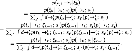
Let S = {s₁, …, s_n} denote the set of species present in the sample. Let t_k be the time at which the k^th photon is detected, and ξ_n = {t₁, …, t_n} denote the set of arrival times in a particular experiment up to time t_n. We wish to find an expression for the probability P(s_j|ξ_k) the probability that at time t_k the signal we are observing is due to a molecule of type s_j (note that we will always use standard probability notation in which—for example—p(A; B|C; D) represents the probability of A and B given C and D; we use P(·) to designate probabilities on strictly discrete spaces and p(·) for probability densities on continuous spaces or joint densities over both discrete and continuous spaces). Since the fluorescence rate is dependent on the (time-correlated) molecular position , we must start with a distribution over species and spatial coordinates . Using Bayes' rule and the definition of conditional probability, we find the following expression for the probability that a molecule is of type s_j and is at position given the observed photon stream ξ_k:

(1)

In our notation the event t_k together with the measurement record ξ_k−1 is symbolically identical to the measurement record ξ_k. For diffusion in d dimensions, the integrals in Eq. 1 are over all of R^d.

We now expand over possible values for to find

(2)

which contains the recursive term . We substitute into Eq. 1 to find a formula for the time evolution of the probability distribution over molecular species s_j and position conditioned on a set of measured fluorescence photon arrival times ξ_k:

(3)

We were required to carry along a distribution over spatial coordinates to develop a recursion formula. In the end, however, we are interested in species identification through the probability P(s_j|ξ_k) which we may now write in terms of Eq. 3 as

(4)

We define our species identification estimator ŝ as the value of s_j ∈ S which maximizes Eq. 4. The estimator ŝ defined by Eqs. 3 and 4 is exact, in the sense that we have not made any assumptions about the correlation between molecular diffusion statistics and photon detection statistics. To update an estimation based on the k^th photon detection at time t_k, we only require knowledge of two distributions, and . The former distribution represents the fluorescence emission statistics of a molecule of type s_j at a particular position in the laser focus, while the latter distribution represents the diffusion statistics of a molecule of type s_j. Next, we will describe explicit functional forms for these distributions which are relevant to confocal microscopy experiments.

Effective diffusion statistics

In a typical experimental situation, the motion of a molecule between points and is not correlated with any photon detection events. This point is somewhat subtle, and relies on our explicit inclusion of both fluorescence and diffusion statistics. If we detect many photons in a small time interval, it is very likely that a fluorescent molecule is at a position of high laser intensity, so that the position of a molecule is correlated with the measurement record ξ_k. However, the future probability that the molecule will move from position to position (without emitting a photon) in time Δt_k ≡ t_k − t_k−1 is independent of the prior photon detections ξ_k−1. Symbolically, we have

(5)

where the right-hand side of Eq. 5 is the usual Green's function solution to a Fokker-Planck equation for the diffusion statistics of molecules of type s_j.

In most cases of experimental interest, we may average over three-dimensional distributions to obtain a set of estimator equations which is effectively two-dimensional. Furthermore, if we consider a cylindrically symmetric laser excitation profile, we may reduce all of the (vector) coordinates to (scalar) cylindrical radial coordinates r_k, where as before r_k ≡ r(t_k). For isotropic, force-free Brownian motion projected into d = 2 dimensions, we can solve Eq. 5 analytically to find

(6)

where D_j is the diffusion coefficient for molecules of type s_j and I₀ is the 0^th-order modified Bessel function of the first kind.

Fluorescence photon detection statistics

Equation 6 contains all of the information we need to know about diffusion to implement the filter, Eq. 3. Next we will develop an explicit expression for the fluorescence photon detection statistics p(t_k|r_k; ξ_k−1; s_j) (we have dropped the vector notation on r_k as before). For simplicity, we use a simple two-level, saturating emitter model of fluorescence, but the implementation of the filter is essentially the same for any rate-equation model or model incorporating the internal dynamics of the fluorophore (Berglund et al., 2002). In this model, the instantaneous rate γ_j(r_k) of photon emission by a molecule of type s_j at position r_k and labeled with m_j (identical) dye molecules is determined by the spatially dependent laser excitation rate Γ_L(r_k), the relaxation rate of the dye molecule Γ_j, and the background noise count rate Γ_B as

(7)

Γ_L(r) is proportional to the laser beam intensity which we take to be Gaussian with beam waist w in the transverse dimensions, and we neglect the variation of the excitation intensity in the axial direction as

(8)

It should be noted here that finite efficiency photon detection does not affect the forms of the filter or the fluorescence model. We can always scale the rates in Eq. 7 by the detection efficiency η which has no effect on the spatial dependence of fluorescence statistics (except to decrease the overall rate of photon detection). Furthermore, for small η, we may assume that a fluorophore emits many photons (∼1/η) between any two photon detections. This ensures that the fluorophore is in its radiative steady state and we may safely neglect any quantum statistics associated with single-molecule photon detection. Since the form of Eq. 3 is largely independent of η, we often neglect the distinction between photon emission and detection rates, whose ratio is η by definition.

The probability 2εp(t_k|r_k; ξ_k−1; s_j) is the likelihood of a photon detection in the infinitesimal interval t_k ± ε with no other photons detected at times t ∈ (t_k−1, t_k). This probability can be expressed as

(9)

where n_k is the number of photons emitted in time interval Δt_k. Note that the precise value of the factor ε is unimportant because exp(−2εγ(r_k)) ≈ 1 since ε is very small by definition. The integral represents an average over all possible starting radial positions r_k−1 from which the molecule moves to radial position r_k in the time interval Δt_k. In general, n_k depends on the path taken by the molecule over the time interval, which makes calculating an exact analytical expression for Eq. 9 difficult, although a path integral representation is possible (see Appendix). The difficulty in calculating this function arises from the variation of the photon emission rate over the possible paths that a molecule can take from r_k−1 to r_k. We expect the fluorescence count to obey Poisson statistics, so

(10)

as long as a molecule does not move between photon detections to a position of very different excitation intensity. We expect the approximation in Eq. 10 to hold for w²γ_j(0) ≫ D_j, so that a molecules does not move too far between photon detections. This is precisely the experimental regime of interest, since this condition is violated when few photons are detected in a single-molecule transit through the laser focus, and we would not expect to gain much information in this case anyway. In the Appendix we calculate the first-order correction to Eq. 10. For typical parameters in our simulations, the numerical value of this correction factor is <2% for regions within the beam waist of the laser.

Practical considerations

Several details must be considered before the filter can actually be implemented. First, while the integrals in Eq. 3 are over all of R^d, we must truncate them numerically. We set the integration limit R_max > w, the laser beam waist, so that Γ_L ≈ 0 in the regions excluded from the integrals; in practice, we find that R_max = 4w is sufficient.

Next, to account for the loss of probability at the boundary R_max due to the diffusion term, we add a distribution representing the probability of molecules from the outer regions diffusing into the region bounded by R_max to the spatial distribution in Eq. 3 at each iteration of the estimator. This takes into account the concentrations of the different species in the sample, and is given by

(11)

which is a convolution of Eq. 6 with the distribution of molecules in the outer region, which we assume to be uniform with concentration C_j. This leak term allows us to run the estimator in the absence of a molecule in the laser focus. To account for the possibility of an empty laser focus, we include a dark species s₀ with brightness m₀ = 0 in all iterations of the estimator. Note that we have not yet defined the initial distribution ; to obtain this distribution we simply run the estimator on background noise, in the absence of fluorescent species, until a steady-state distribution is reached.

Finally, we must decide how to determine when a molecule has either entered or exited the laser focus. For this we use the spatial distributions generated by the estimator. We decide on a particular threshold radius R_th that bounds what we consider to be the laser focus, and calculate the probability that the focus is empty,

(12)

We decide on a minimum value P_low for this probability and consider a molecule to have entered the laser focus when Eq. 12 drops below this value. Additionally we choose a maximum value P_high and consider the molecule to have exited the focus when Eq. 12 increases above P_high. At this point, we integrate the spatial distributions to obtain an estimate of the identity of the observed molecule. We leave detailed discussion of the motivation for this scheme to a future publication.

With these details specified, our formulation of the estimator is complete. Next, we discuss the expected strengths and limitations of the estimator under particular experimental conditions.

Experimental regimes

While the derivation of Eq. 3 is applicable to all cases of molecular diffusion and fluorescence, we expect its performance to be affected by the parameters of the experiment. For instance, we stated that Eq. 10 is a poor approximation when the diffusion rate is very fast relative to the fluorescence rate . We may attempt to evaluate Eq. 9 more accurately, but the performance of our estimator will still be quite limited due to its dependence on a spatial distribution that changes more rapidly than it is updated. We expect the filter to be most effective when is high and diffusion rate is low, so that the value we calculate for remains a good estimate for as the molecule moves from to .

It may be the case that the diffusion rate is very small relative to γ_j—such is the case for diffusion of molecules on a membrane, for example. In this case we expect to detect large numbers of photons at a fairly constant rate, so that little spatial information is gained from the time spacing between photons. Hence we expect that we can ignore this spacing and the exact arrival-time data, and instead count the numbers of photons detected in individually spaced time bins of arbitrary size τ_bin. Then we replace ξ_k = {t₁, …, t_k} with ξ_k = {n₁, …, n_k} in deriving Eq. 3, where we define n_k as the number of photons counted in the time bin (t_k−1, t_k). We define as before. Here the diffusion probabilities are calculated as in Eq. 5, and the fluorescence probabilities are calculated using

(13)

where the approximation, as in Eq. 10, comes from the molecule's path-dependent fluorescence rate.

This formulation of the estimator requires significantly fewer computations, because the diffusion and fluorescence probabilities can all be calculated before the experiment, making real-time estimation easier to achieve. We expect the performance to be determined in part by the bin time τ_bin that we choose—a τ_bin that is too large ignores significant diffusion dynamics, but more computations are required as the bin time is made smaller—so the choice of bin time requires balancing these tradeoffs.

Generalizing the approach

We have stated that the most important point that we are presenting here is a general approach to computational single-molecule studies. It is important, then, to consider how our approach generalizes to other experiments. The recursive estimator given by Eq. 3 is a valid form for any experiment in which no more than a single molecule is likely to be in the focus of the laser; modifications or extensions of the models for diffusion and fluorescence do not affect the form of the estimator. Obvious extensions to the fluorescence model may incorporate multiple spectral channels to facilitate further identification or experiments using fluorescence transfer (Berglund et al., 2002). Additionally, more fluorescence details may be incorporated if necessary, such as dye photobleaching, blinking dyes, forbidden transitions, and spatially dependent photon collection efficiency. Extensions to the diffusion model can be made to incorporate diffusion restricted to a particular spatial domain, diffusion with net flow, and as we have stated, free diffusion in higher or lower dimensions. Clearly this makes feasible the use of this recursive estimator in many common chemical and biological experiments.

As stated earlier, parameter estimation can be treated as an extension of identification as we have defined it here. Any parameter that can be incorporated into our model for identification can also be approximated by our technique if we simply perform identification over a set in which that parameter is varied—this is precisely a maximum likelihood estimator (see Degroot, 1986, for example). It is also possible to use a similar approach to derive estimators for parameters that are relevant on the bulk sample scale, not the single-molecule scale. For example, the details of single-molecule observations are not affected by sample concentration, although the frequency of such observations is. It is not very difficult to write a concentration estimator using a model for this frequency. Coupled with the identification estimator, this could be used to estimate the concentrations of the different components of a sample. Thus all of the functionality of FCS and other current techniques can be achieved by rigorous estimation and extended to include any exotic photophysical or diffusion dynamics for which a suitable model exists.

Our ultimate goal is the development of techniques that facilitate experiments in which exotic dynamics will limit the efficacy of current methods. Current techniques are limited to experiments for which sufficient autocorrelation functions or histograms can be generated for fitting to the experimental data. We envision experiments in which fluctuations in the quantities being measured affect the fluorescence stream in such a way that realizing accurate results by fitting observations to a small number of sample functions will be impossible. For example, to study time-dependent mechanical oscillations or rotations in single molecules—such oscillations are common to proteins yet current techniques for their study are quite limited (Bao and Suresh, 2003)—an FCS experiment would require an enormous number of model autocorrelations to explore a significant portion of the infinite dimensional space that such oscillations lie in. In contrast, with an appropriate model our recursive update approach would be capable of making a statistically best estimate of the oscillatory state of such a system continuously in time for as long as the system can be observed. We can also imagine the study of random events that have a dramatic effect on diffusion dynamics, such as active intercompartmental transport of free molecules in a living cell, in which there is not only a random short-duration change in the diffusion coefficient during transport, but also a change in the topology of the space over which the molecule is confined. Again, for such a process it will be very difficult to calculate or simulate a sufficient set of functions to fit the observations to, while a recursive update formula with a sufficient model can be readily written down. We believe our approach is the best path to take for the study of such complex stochastic single-molecule dynamics.

Now we will present the results of simulations to demonstrate and characterize the estimator in the single-molecule identification experiment.

SIMULATIONS

In this section, we will simulate diffusion experiments in two dimensions in MATLAB to illustrate the use of the recursive filtering technique for the analysis of photon streams (for computer code to implement the estimator, please contact the authors). The simulations specify a set S of species with varied diffusion coefficients D_j and brightness m_j, and all other model parameters held constant. Discrete, fine-grained (Δt = 0.5 μs) Brownian motion trajectories are generated for a particular species, and photon streams are generated from a Poisson distribution with rate given by Eq. 7. We set the beam waist w = 0.5 μm and rates Γ_L(0) = 637 ms⁻¹ and Γ_j = 500 ms⁻¹ for all j. We first set Γ_B = 1 kHz to evaluate the estimator in the presence of minimal background noise. The arrival times of photons are extracted from the stream and sent to the estimator for evaluation, and identifications are made from the resulting distributions using R_max = 2 μm, R_th = w = 0.5 μm, P_low = 0.25, and P_high = 0.75.

Identification based on diffusion coefficient

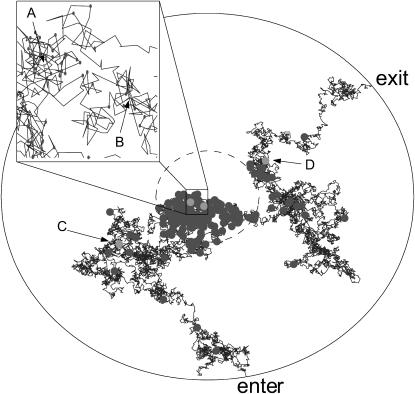
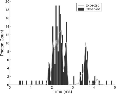
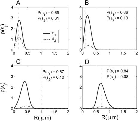
An experiment that we may perform using our identification algorithm is one in which the dye-labeled sample molecules may polymerize with unlabeled molecules, and we try to distinguish between monomers and dimers. For example, such an experiment could be used to distinguish between single-stranded and double-stranded DNA. Figs. 1 and 2 show a sample trajectory and photon stream generated for an experiment with S = {(1, 0.25), (1, 0.5)} where we denote s_j = (m_j, D_j) with D_j in units of μm²/ms; these values are consistent with small nucleic acid polymers (Doi and Edwards, 1986; Laurence et al., 2004). The trajectory shown is for a molecule of type s₁. This photon stream was run through the estimator and some of the resulting spatial distributions are shown in Fig. 3. We see in these distributions the effect that random fluctuations can play in the estimate—whereas the peaks of the spatial distributions for the molecule at positions A, B, and D are nearly exactly at the molecule's actual radial position, the estimator is off by nearly one beam waist when the molecule is at position C. Statistically, such momentary inaccuracies are expected; by its recursive nature, however, the estimator corrects such errors quickly as additional photons are detected.

FIGURE 1.

Data generated by two-dimensional simulation. The plot shows a trajectory of a molecule with D_j = 0.25 μm²/ms and m_j = 1 through the circular region centered at the laser focus with radius R_max = 2 μm. The inner, dashed circle represents the laser beam waist. Entry and exit points are indicated. Displayed molecule positions are updated in 0.5-μs increments. Circles indicate the molecule's position at each photon arrival time. Labeled points correspond to the times at which the distributions in Fig. 3 are shown.

FIGURE 2.

Simulated photon counts detected in time intervals of 50 μs as the molecule traversed the path in Fig. 1. Also shown is the expected photon count over these intervals based on the actual laser intensity at the molecule's position, given by Eq. 7. Note the difference between expected and detected fluorescence rates—this contributes to the difficulty of extracting accurate spatial information from the photon stream.

FIGURE 3.

Sample spatial distributions resulting from the stream of 253 photons presented in Fig. 2, using S = {(1, 0.25), (1, 0.5)}. The distribution after the 62nd photon detected (point A in the trajectory) is in the top left. The top right, bottom left, and bottom right distributions are after the 125th, 188th, and 252nd photons, with the molecule at positions B, C, and D, respectively. Integrated probabilities given by Eq. 4 are reported for each species. Dotted vertical lines indicate the actual radial position of the molecule.

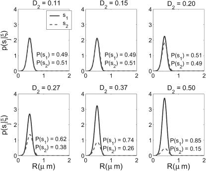
To evaluate the performance of the recursive estimator in this type of experiment over a range of possible S, we vary the ratio of diffusion coefficients between species: we set S = {(1, 0.1), (1, D₂)} with 0.1 ≤ D₂ ≤ 0.5. Fig. 4 shows the final probability distributions over space and species type for a single simulated trajectory and set of photon arrival times for a molecule of type s₁, run through the estimator with varied values for D₂. This highlights an important aspect of the estimator: in addition to providing an identification scheme, it provides a quantitative evaluation of the accuracy of the identification in the form of the probability that the estimated species is indeed present. The estimator was not able to correctly identify the molecule for D₂ ≤ 0.15, however; as D₂ increased to 0.5, P(s₁|ξ) increased to 85%.

FIGURE 4.

Performance of recursive estimator in identifying species with varied diffusion coefficient ratios. One trajectory and resulting set of 91 photon arrivals was generated for molecule type s₁ with the set S = {(1, 0.1), (1, D₂)}, for six logarithmically spaced values of D₂. Shown are the radial distributions for each species after the final photon arrival time was processed. Integrated probabilities are indicated.

We now consider the accuracy of the estimator in identifying molecules relative to theoretical upper and lower performance bounds. A primary difficulty in extracting information about the diffusion dynamics lies in the uncertainty in estimating molecule position from fluorescence rate, since the detected fluorescence rate is not a deterministic function of position (see Fig. 2). In theory, the best possible identification estimate could be made if the exact position of the molecule could be extracted from the data at each iteration of the estimator. To simulate this we generate trajectories and photon streams in a manner identical to that used for the recursive estimator, but we record the exact radial position of the molecule at every photon arrival time. We use a maximum likelihood estimator (see Degroot, 1986, for an example) for species identity from the position and arrival-time data; we take the probability of successful identification by this method to be the theoretical upper bound for performance in any simulated experiment. In addition, we decide on a lower bound for the success probability by considering only the duration of the identification trajectory—this should contain the least possible information about the diffusion dynamics. We numerically approximate p(τ|D_j), the probability distribution of the time τ spent within the laser focus given the diffusion coefficient D_j, and let our identification estimate for each trajectory be the species for which this probability is greatest. We take the performance of such an estimator to be the minimal performance that we should be able to achieve with data from a single trajectory.

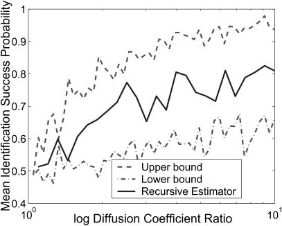
Fig. 5 compares the accuracy of the recursive estimator to that of the theoretical upper and lower bounds. For clarity, success probabilities are not shown for each species, but rather the geometric mean of the two probabilities is shown. The geometric mean was chosen as a simple measure of both the accuracy and the bias of the estimator; it is highest only when the estimator is nearly unbiased and accurate for both species. For diffusion coefficient ratios less than 1.5, the probability of successful identification lies near 50% for all three estimators. For ratios greater than 1.5, the recursive estimator lies well within the bounds. Note that here we only consider the probability that the estimator correctly reports the species present, not the reported probability of the estimate. We expect to be able to improve the performance by specifying a minimum threshold for this probability and thereby only accepting estimates that are made with a high degree of certainty; these data represent a minimal level of performance for our estimator.

FIGURE 5.

The performance of the recursive estimator as a function of diffusion coefficient ratio, compared to that of the estimators representing theoretical upper and lower performance bounds. We set S = {(1, 0.1), (1, D₂)} and generate trajectories resulting in at least 200 identifications for each species type, for each estimator, for varied D₂. Plotted are the geometric mean success probabilities for each estimator.

Identification of diffusing fluorophores by diffusion coefficient alone is a problem addressed by FCS. Using this method, a nonlinear fit to simulated data or a maximum likelihood estimator is used to identify a species given its autocorrelation function (Enderlein and Köllner, 1998). Our technique has several advantages over this method, in that the estimator provides a rigorous probability distribution over species present in the sample. Thus in addition to a most probable identity, it provides a measure of how certain the estimate can be considered to be. In addition, such an estimate can be made at any time during the fluorophore's path through the beam focus, allowing an experiment to interact with sample molecules before they leave the focus, as is necessary for a tracking or sorting experiment. FCS methods, in contrast, rely on an autocorrelation that may not provide a good identification estimate with incomplete data. Of course, a major advantage over FCS is that we can consider additional molecular parameters in our identifications. Next we consider an experiment in which the species present may differ in brightness m_j.

Multiple species identification

Here we propose a hypothetical experiment in which four dye-labeled species exist in solution: one small molecule, one large molecule, one small-large molecule complex, and one small-large complex where one of the dyes has photobleached. Such experiment could be useful if, for instance, we wanted to measure the kinetics of complex formation. We can also imagine an experiment using real-time feedback to isolate only the complex with two intact dyes from solution. To simulate such experiments, we let S = {(1, 0.4), (1, 0.2), (1, 0.15), (2, 0.15)} to test low diffusion coefficient ratios and S = {(1, 2), (1, 0.4), (1, 0.08), (2, 0.08)} to test high ratios. The ratios between molecular diffusion coefficients of complexes and their constituents are largely dependent on the relationships between the geometry of the individual components and that of the complex. Hence both cases have some physical relevance, with the low-ratio case an example where geometry is largely not altered by binding, and the high-ratio case an example in which the individual constituents may be tightly folded, for instance, while the complex takes a large, extended form.

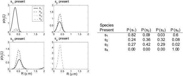
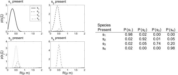
Figs. 6 and 7 show distributions resulting from trajectories generated by each species type in the multiple species experiments. In the low diffusion coefficient ratio experiments, the estimator identifies s₁ and s₄ with high probability, but cannot distinguish well between s₂ and s₃ due to their very similar diffusion coefficients. For higher diffusion coefficient ratios, all species are identified with high probability. Note that in both cases, s₄ is identified with probability nearly 1, indicating that brightness is a much stronger criterion for distinguishing between species than diffusion coefficient.

FIGURE 6.

(Left) The performance of the recursive estimator in the multiple component experiment with S = {(1, 0.4), (1, 0.2), (1, 0.15), (2, 0.15)}. Trajectories were generated for each species, and the resulting photon arrival-time data was run through the estimator. The distributions shown are the distributions before the final exit time of the molecule for each trajectory. (Right) The table shows the integrals of the probability distributions shown in the figure, giving the probability of each species being present according to the data generating each plot.

FIGURE 7.

(Left) The performance of the recursive estimator in a high diffusion coefficient ratio multiple component experiment with S = {(1, 2), (1, 0.4), (1, 0.08), (2, 0.08)}. Trajectories were generated for each species, and the resulting photon arrival-time data was run through the estimator. The distributions shown are the distributions before the final exit time of the molecule for each trajectory. (Right) The table shows the integrals of the probability distributions shown in the figure, giving the probability of each species being present according to the data generating each plot.

Experiments to distinguish between species based on both diffusion coefficient and brightness are the focus of the FIMDA and PAID methods (Laurence et al., 2004; Palo et al., 2000). Our method has several advantages over these. Again, our estimator reports identification probability, a rigorous measure of the confidence in the estimate. This is useful in any experiment—for kinetics experiments, we can calculate the appropriate uncertainties in whatever values we measure; for sorting, we can be highly certain that we extract the correct molecules. Second, FIMDA and PAID require multidimensional nonlinear fits of their data to simulated or theoretical results, making real-time experiments nearly impossible with modern computer hardware. Third, as in the comparison with FCS, our technique always provides the statistically best estimate of the species present at all times, providing information for real-time experiments while the fluorophores are within the focal volume. While we are not aware of any studies that examine the performance of FIMDA and PAID in the identification of single diffusing molecules, we expect that our estimator should be at least as accurate as these methods.

Slow-diffusion identification

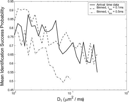
In experiments where species diffusion coefficients are small relative to the fluorescence rates, we expect that a reduction of the photon stream from a series of arrival times to a series of photon counts in time windows of length τ_bin will be both effective and computationally simpler than the arrival-time estimator that we have been using. We test this by running a series of two-species diffusion-based identification simulations, setting S = {(1, D₁) (1, 3D₁)} and varying D₁. Fig. 8 shows the results of these simulations, run using bin times of 0.1 ms and 0.5 ms. We see that for small diffusion coefficients, with sufficiently small bin time, the binned-data estimator's performance reaches as high as 90%—roughly 10 percentage points higher than the performance of the arrival-time estimator. For D₁ ≥ 0.02 μm²/ms, both estimators achieve roughly the same performance. When a larger bin time is used, the performance of the binned-data estimator is degraded, falling as low as 50% before the data become too coarse-grained to make identifications, which happens for D₂ > 0.3 μm²/ms.

FIGURE 8.

Comparison of estimator performance using binned photon-count data and arrival-time data. Geometric mean success probabilities are shown for simulations in which we set S = {(1, D₁), (1, 3D₁)} and vary D₁. A minimum of 100 identifications was made for each species, for each value of D₁, for both estimators. Binned data were generated with bin times τ_bin = 0.1 ms and τ_bin = 0.5 ms, as indicated in the legend. For τ_bin = 0.5 ms, the estimator cannot successfully observe species s₂ for D₃ > 0.3 μm²/ms, so the plot does not continue beyond this point.

It is somewhat surprising to see the binned-data estimator outperform the exact arrival-time estimator. We attribute this result to accumulated numerical error as many photon arrival times are processed; finite precision mathematics (MATLAB uses 64-bit data types) limits the accuracy of each iteration of the estimator. The binned-data estimator may update as little as 10% as frequently as the arrival-time estimator, and as a result the difference in accumulated error is great enough that the binned estimator performs better despite the arrival-time estimator's theoretical advantage. The effect is particularly pronounced for molecules with small diffusion coefficients because a very large number of photons is typically detected as such molecules diffuse through the laser focus. This results in a large number of recursive updates, each introducing some numerical error to the distribution.

As shown in Fig. 8, the performance of the binned-data estimator will be limited by selection of the bin time; to achieve best results, the bin time must be made sufficiently small to capture essential features of the fluorescence stream, yet not too small to cause numerical error to hurt accuracy. Initial speculation about the implementation of the recursive estimator on a field programmable gate array (Stockton et al., 2002) leads us to believe that the binned-data estimator with reasonable bin time reduces the frequency of computations sufficiently to enable its use in experiments requiring real-time feedback.

Clearly the binned-data estimator, not the arrival-time estimator, is the best tool for the current problem both for computational efficiency and accuracy, at least when numerical precision is limited to 64-bit. However, the arrival-time formulation will be essential for experiments in which fast photophysical dynamics, such as blinking or energy transfer, are incorporated into the fluorescence model. The binned-data estimator will never be able to accurately handle dynamics on a timescale smaller than τ_bin, whereas the arrival-time estimator's time resolution is limited only by photodetector resolution.

Background noise and estimator performance

So far we have only presented results showing the performance of the estimator with 1 kHz background noise. Here we consider the effect of higher-rate background fluorescence on the estimator. The model that we derived for the fluorescence incorporated a constant rate background count Γ_B. We expect that Eq. 7 will provide fluorescence rates that are exact assuming that the noise has a constant rate that can be measured or approximated before the experiment.

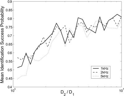
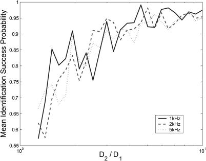
Figs. 9 and 10 show the identification accuracy of the estimator on data containing constant-rate Poisson background noise. The plots are generated by setting S = {(1, D₁), (1, D₂)} with D₁ constant at 0.1 for the arrival-time data and 0.01 for binned data, and varying the ratio D₂/D₁. Note that a direct comparison between the probabilities in these figures is irrelevant because the plots are over different diffusion coefficient regimes. We see that there is little noticeable difference in the performance of the estimator on either data type with noise at 1 kHz and 2 kHz, but for noise strengths of 5 kHz there is a performance loss of a few percentage points for the arrival-time data. The difference in noise-rejection performance between the data types is again attributed to numerical issues: higher noise count rates increase the number of iterations of the arrival-time estimator and therefore increase propagated error. A typical experimental apparatus is capable of a background count rate of 1–2 kHz, and both estimators successfully handle noise at these levels (Berglund et al., 2002; Enderlein and Sauer, 2001).

FIGURE 9.

Performance of the arrival-time estimator on data with varied background noise strengths indicated. The plots were generated using S = {(1, 0.1), (1, D₂)}, and 0.1 < D₂ ≤ 1.0, with a minimum of 200 identifications made for each species. Data shown are the geometric means of the success probabilities for each species.

FIGURE 10.

Performance of the identification estimator on binned data with bin time 0.1 ms and varied background noise strengths as indicated. The plots were generated with S = {(1, 0.01), (1, D₂)}, and 0.01 < D₂ ≤ 0.1, with at least 100 identifications made for each species. Shown are the geometric means of the success probabilities for each species.

CONCLUSION

We derived a recursive Bayesian estimator to calculate a probability distribution for the identity of a single diffusing fluorophore given its photon arrival-time stream as it makes a single pass through the focus of a confocal fluorescence microscope. We derived analytical models for the diffusion and fluorescence dynamics in such an experiment, and tested our estimator by running experimental simulations in two dimensions.

We showed that our estimator is capable of identifying single molecules based on differences in their diffusion coefficients and brightness, but we stress that our method provides a means of identification that is based on any species-specific parameter. Our simulations indicated that the accuracy of the estimator in identification by diffusion coefficient is reasonable, as it lies within the performance bounds set by a minimal-data estimator and an ideal, theoretical one. We showed that our estimator is significantly more sensitive to brightness than it is to diffusion coefficient by demonstrating that species with twofold differences in brightness can be identified with probability 1, whereas estimator accuracy on species with twofold differences in diffusion coefficient is not much better than random guessing.

A key feature of our identification scheme is that it provides a probability distribution over the set of possible species identities. This provides a measure of the certainty of an identification, as we demonstrated that relatively similar species are identified with fairly low probability, and relatively dissimilar ones are identified with high probability.

We showed that by counting photon arrivals in time windows of fixed duration we can significantly reduce the number of calculations necessary while maintaining accuracy in diffusion coefficient-based identification for slowly diffusing molecules. In fact, accuracy improved by doing this because of issues with the accumulation of numerical errors over many estimator iterations. We believe that this approach is experimentally tractable, in that it is both accurate and computationally simple enough to facilitate experiments requiring real-time feedback.

It is important to note that our work was done in two dimensions purely for computational simplicity and to illustrate the technique. The estimator is valid in an arbitrary number of dimensions, and the models we derived are easily extended to three dimensions. Assuming a correct model, we believe that the performance of the estimator applied in three dimensions will not be much different than that which we have presented.

The most important point we wish to address is the prospect of using approaches similar to what we have presented to tackle more complicated problems in single-molecule spectroscopy. Rigorous mathematical tools exist for the treatment of stochastic processes such as diffusion and fluorescence, and when applied properly they yield direct quantitative approaches to the same problems that have previously been addressed using more limited and circuitous methods. These quantitative tools are only limited in the extent to which the physical processes underlying the experiments are understood; for any system that we can write an accurate model for, we can develop an estimator to measure something about that system. We hope we have made clear the motivation for our belief that coupling a rigorous quantitative approach to data analysis with clever experiments will allow for novel studies of complex stochastic dynamics on the single-molecule scale.

APPENDIX

Perturbative calculation of p(n_k = 0|r_k; r_k−1; ξ_k; s_j)

Let be a position-dependent Poisson rate with as some fixed path satisfying and . Let be the probability that no photon is emitted along the path . From an elementary probability calculation, we have

(14)

where the notation is to indicate that p₋ is a functional of the path .

p(n_k = 0|r_k; r_k−1; ξ_k; s_j) is the average of the functional over all (scalar) paths r(t) with r(0) = r_k−1 and r(t) = r_k. Since the sample paths are generated by Brownian motion, we take the Wiener measure dμ_W[r(t)] with diffusion coefficient D_j as our probability measure on this function space (Chaichian and Demichev, 2001). We may now write p(n_k = 0|r_k; r_k−1; ξ_k; s_j) as a path integral over the class F of all continuous functions from (r_k−1, t_k−1) to (r_k, t_k) as

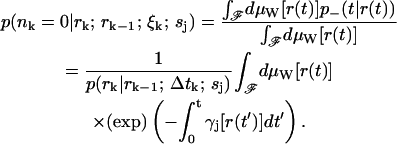(15)

If we now write the instantaneous rate function as

(16)

where

(17)

we may make a perturbation expansion of Eq. 15 around the constant potential .

For the constant rate , we have

(18)

Including the first-order contribution from the perturbing term gives the next lowest-order correction of

(19)

References

- Bao, G., and S. Suresh. 2003. Cell and molecular mechanics of biological materials. Nature Mat. 2:715–725. [DOI] [PubMed] [Google Scholar]
- Berglund, A. J., A. C. Doherty, and H. Mabuchi. 2002. Photon statistics and dynamics of fluorescence resonance energy transfer. Phys. Rev. Lett. 89:068101. [DOI] [PubMed] [Google Scholar]
- Böhmer, M., and J. Enderlein. 2003. Fluorescence spectroscopy of single molecules under ambient conditions: methodology and technology. Chem. Phys. Chem. 4:792–808. [DOI] [PubMed] [Google Scholar]
- Chaichian, M., and A. Demichev. 2001. Path Integrals in Physics, Volume I: Stochastic Processes and Quantum Mechanics. Series in Mathematical and Computational Physics. IOP Publishing, London, UK.
- Chen, Y., J. D. Müller, P. T. So, and E. Gratton. 1999. The photon counting histogram in fluorescence fluctuation spectroscopy. Biophys. J. 77:553–567. [DOI] [PMC free article] [PubMed] [Google Scholar]
- Degroot, M. H. 1986. Probability and Statistics. Addison-Wesley, Reading, MA.
- Doi, M., and S. F. Edwards. 1986. The Theory of Polymer Dynamics. International Series of Monographs on Physics. Clarendon Press, Oxford, UK.
- Dörre, K., S. Brakmann, M. Brinkmeier, K.-T. Han, K. Riebeseel, P. Schwille, J. Stephan, T. Wetzel, M. Lapczyna, M. Stuke, R. Bader, M. Hinz, H. Seliger, J. Holm, M. Eigen, and R. Rigler. 1997. Techniques for single molecule sequencing. Bioimaging. 5:139–152. [Google Scholar]
- Eigen, M., and R. Rigler. 1994. Sorting single molecules: application to diagnostics and evolutionary biotechnology. Proc. Natl. Acad. Sci. USA. 91:5740–5747. [DOI] [PMC free article] [PubMed] [Google Scholar]
- Elson, E. L. 2001. Fluorescence correlation spectroscopy measures molecular transport in cells. Traffic. 2:789–796. [DOI] [PubMed] [Google Scholar]
- Elson, E. L., and D. Magde. 1974. Fluorescence correlation spectroscopy. I. Conceptual basis and theory. Biopolymers. 13:1–27. [DOI] [PubMed] [Google Scholar]
- Enderlein, J., and M. Köllner. 1998. Comparison between time-correlated single photon counting and fluorescence correlation spectroscopy in single molecule identification. Bioimaging. 6:3–13. [Google Scholar]
- Enderlein, J., and M. Sauer. 2001. Optimal algorithm for single-molecule identification with time-correlated single-photon counting. J. Phys. Chem. A. 105:48–53. [Google Scholar]
- Goodwin, P. M., W. P. Ambrose, and R. A. Keller. 1996. Single-molecule detection in liquids by laser-induced fluorescence. Acc. Chem. Res. 29:607–613. [Google Scholar]
- Hess, S. T., S. Huang, A. Heikal, and W. W. Webb. 2002. Biological and chemical applications of fluorescence correlation spectroscopy: a review. Biochemistry. 41:697–705. [DOI] [PubMed] [Google Scholar]
- Kask, P., K. Palo, N. Fay, L. Brand, U. Mets, D. Ullmann, J. Jungmann, J. Pschorr, and K. Gall. 2000. Two-dimensional fluorescence intensity distribution analysis: theory and applications. Biophys. J. 78:1703–1713. [DOI] [PMC free article] [PubMed] [Google Scholar]
- Kask, P., K. Palo, D. Ullmann, and K. Gall. 1999. Fluorescence-intensity distribution analysis and its application in biomolecular detection technology. Proc. Natl. Acad. Sci. USA. 96:13756–13761. [DOI] [PMC free article] [PubMed] [Google Scholar]
- Laurence, T. A., A. N. Kapanidis, X. Kong, D. S. Chemla, and S. Weiss. 2004. Photon-arrival-time interval distribution (PAID): a novel tool for analyzing molecular interactions. J. Phys. Chem. B. 108:3051–3067. [Google Scholar]
- Lipman, E. A., B. Schuler, O. Bakajin, and W. A. Eaton. 2003. Single-molecule measurement of protein folding kinetics. Science. 301:1233–1235. [DOI] [PubMed] [Google Scholar]
- Magde, D., E. Elson, and W. W. Webb. 1972. Thermodynamic fluctuations in a reacting system—measurement by fluorescence correlation spectroscopy. Phys. Rev. Lett. 29:705–708. [Google Scholar]
- Maiti, S., U. Haupts, and W. W. Webb. 1997. Fluorescence correlation spectroscopy: diagnostics for sparse molecules. Proc. Natl. Acad. Sci. USA. 94:11753–11757. [DOI] [PMC free article] [PubMed] [Google Scholar]
- Palo, K., U. Mets, S. Jäger, P. Kask, and K. Gall. 2000. Fluorescence intensity multiple distributions analysis: concurrent determination of diffusion times and molecular brightness. Biophys. J. 79:2858–2866. [DOI] [PMC free article] [PubMed] [Google Scholar]
- Prummer, M., C. Hübner, B. Sick, B. Hecht, A. Renn, and U. P. Wild. 2000. Single-molecule identification by spectrally and time-resolved fluorescence detection. Anal. Chem. 72:443–447. [DOI] [PubMed] [Google Scholar]
- Rarbach, M., U. Kettling, A. Koltermann, and M. Eigen. 2001. Dual-color fluorescence cross-correlation spectroscopy for monitoring the kinetics of enzyme-catalyzed reactions. Methods. 24:104–116. [DOI] [PubMed] [Google Scholar]
- Schwille, P., and U. Kettling. 2001. Analyzing single protein molecules using optical methods. Curr. Opin. Biotechnol. 12:382–386. [DOI] [PubMed] [Google Scholar]
- Stockton, J., M. Armen, and H. Mabuchi. 2002. Programmable logic devices in experimental quantum optics. J. Opt. Soc. Am. B. 19:3019–3027. [Google Scholar]
- Weiss, S. 1999. Fluorescence spectroscopy of single biomolecules. Science. 283:1676–1683. [DOI] [PubMed] [Google Scholar]
- Weiss, S. 2000. Measuring conformational dynamics of biomolecules by single molecule fluorescence spectroscopy. Nat. Struct. Biol. 7:724–729. [DOI] [PubMed] [Google Scholar]