Effects of Receptor Interaction in Bacterial Chemotaxis

Abstract

Signaling in bacterial chemotaxis is mediated by several types of transmembrane chemoreceptors. The chemoreceptors form tight polar clusters whose functions are of great biological interest. Here, we study the general properties of a chemotaxis model that includes interaction between neighboring chemoreceptors within a receptor cluster and the appropriate receptor methylation and demethylation dynamics to maintain (near) perfect adaptation. We find that, depending on the receptor coupling strength, there are two steady-state phases in the model: a stationary phase and an oscillatory phase. The mechanism for the existence of the two phases is understood analytically. Two important phenomena in transient response, the overshoot in response to a pulse stimulus and the high gain in response to sustained changes in external ligand concentrations, can be explained in our model, and the mechanisms for these two seemingly different phenomena are found to be closely related. The model also naturally accounts for several key in vitro response experiments and the recent in vivo fluorescence resonance energy transfer experiments for various mutant strains. Quantitatively, our study reveals possible choices of parameters for fitting the existing experiments and suggests future experiments to test the model predictions.

INTRODUCTION

Bacterial chemotaxis is one of the best-studied biological systems (Berg, 2000). It is the sensory system used by coliform bacteria, such as Escherichia coli, to detect and react to external chemical signals, such as nutrients or toxins. Each E. coli cell is propelled by the rotation of several flagella. The rod-shaped cell moves by two types of motion: “running”, when all the flagella rotate counterclockwise to form a coherent bundle and drive the cell in a straight motion, and “tumbling”, when one or a few of the flagella rotate clockwise and the cell wiggles locally with the net result of changing its orientation. Through years of persistent, innovative studies using physics, chemistry, molecular biology, and genetics methods (Adler, 1976; Berg, 2000; Bren and Eisenbach, 2000; Falke and Hazelbauer, 2001), we now have a fairly complete picture of which molecules are involved and how they interact with each other to receive and react to the external signal. The combination of rich, interesting behaviors of the system, together with the rather complete qualitative knowledge about the underlying pathway, provides us with a unique opportunity to understand a biological system from a more quantitative, systems-level point of view. Indeed, the bacterial chemotaxis system has served as a very useful model system in investigating general principles in biology, such as robustness in biological networks (Barkai and Leibler, 1997; Alon et al., 1999; Yi et al., 2000; Mello and Tu, 2003a). In this article, we focus on another interesting aspect of the system, the interaction between receptors and its effects on the response of the system, such as signal amplification.

There are five types of transmembrane chemoreceptors, capable of binding to different types of external small molecules (ligands). The cytoplasmic part of the receptor forms a complex with a histidine kinase (CheA) through a linker molecule (CheW). The ligand concentration is sensed by the binding of the ligand to the corresponding type of receptor; this information, i.e., receptor bound or unbound to ligand, is passed into the cytoplasm through its effect on the kinase activity of CheA. Upon activation by receptor binding to repellent (or removal of attractant), CheA acquires a phosphate group through autophosphorylation. Once phosphorylated, CheA-P passes its phosphate group to a diffusible signaling protein CheY, which relays the signal from the receptors to the flagellar motors through diffusion inside the cytoplasm. The binding of CheY-P to the FliM ring of the flagellar motor complex biases the flagellar rotation toward clockwise and therefore increases the probability of tumbling. This chain of reactions constitute the “linear” information passage of the signaling pathway. As with almost all other sensory systems, bacterial chemotaxis pathway also regulates the signal by adapting to persistent environmental conditions to permit a large dynamical range of response. The adaptation in bacterial chemotaxis is achieved by a slow modification of the receptors, catalyzed by CheR and CheB for the methylation and demethylation processes, respectively. Each receptor has four methylation sites, and receptors with higher methylation levels generally induce higher kinase activity in the attached CheA.

The natural question for such a qualitatively well-characterized system is whether it can be described at a more quantitative level and what extra insight can be gained from such a quantitative description. Indeed, this question can be meaningfully addressed in bacterial chemotaxis, mainly because quantitative data such as the cell behavior and various biochemical measurements of the system are readily available. More advanced technologies, such as in vivo protein concentration measurements (Sourjik and Berg, 2000, 2002a,b) and single cell response measurements (Cluzel et al., 2000), are also becoming accessible. However, for a complicated system like bacterial chemotaxis, possessing much quantitative data does not automatically lead to a deeper understanding of the system. Most of the experiments are measurements of the response of the system to various external stimuli, for different genetically altered bacterial strains and under different experimental conditions. The complicated interactions between the molecules involved often cause difficulty in interpreting the data and reconciling the results from different experiments. To best use these quantitative data, it is absolutely critical to have a quantitative integrative model of the system that is compatible with the details of the experiments. Only through fitting and understanding various quantitative data within a general model framework can we extract useful information out of the diverse sets of data and achieve a higher level of understanding for bacterial chemotaxis.

One of the most intriguing problems in bacterial chemotaxis is the origin of the large gain in signal transduction. It is observed that for a small fractional change in external ligand concentration, the fractional change in the kinase activity is much larger (Berg and Tedesco, 1975). One idea to explain this phenomena, due to Dennis Bray and his co-workers (Bray et al., 1998), is that the gain could come from receptor coupling. This suggestion is motivated by the fact that the receptors form clusters on the cell membrane (Maddock and Shapiro, 1993). The subsequent modeling efforts (Duke and Bray, 1999; Shi and Duke, 1998; Shi, 2000) were very helpful in confirming the relevance of receptor coupling theoretically, but they could not go beyond the conceptual level due to lack of direct quantitative data. Recently, by using fluorescence resonance energy transfer, Sourjik and Berg (SB) were able to measure the CheY-P concentration in vivo in response to different stimulus levels for both wild-type (WT) and different mutant strains. Following these experiments, we proposed a model to understand the receptor sensitivity and the gain of the system (Mello and Tu, 2003b). Using this model, we were able to fit, using relatively few parameters, the recent in vivo response experiments of Sourjik and Berg for six different strains of mutants. Using the same model, we also showed a possible mechanism for the high gain and high sensitivity for a large range of ambient ligand concentrations for the WT cell. In fitting the SB data within our model, we demonstrated the importance of receptor coupling in general and the existence of strong interaction between different types of chemoreceptors, such as strong interaction between Tsr and Tar, which is consistent with the findings of recent cross-linking experiments (Ames et al., 2002; Ames and Parkinson, 2004).

Although our previous study was specially aimed at explaining the SB experiments, the same model framework can be used to study other experiments. To do that, we need to understand the general properties of this class of models. In this article, we define such a model (slightly different from the one we used in Mello and Tu, 2003b) and study its general properties, including the steady-state properties of the system and the transient response to various stimuli (step or pulse), for both mutant models where methylation and/or demethylation processes are blocked and (WT) models where receptors have a distribution of methylation levels due to methylation/demethylation kinetics. (In this study, WT model refers to any model where methylation/demethylation is included.) The emphasis is twofold here. First, we want to make connections between the general behavior of the model and the experiments and understand the reason behind the agreement or disagreement; second, we want to understand the range and limitations of the model with the purpose of better calibration of the parameters and possible modification of the model itself.

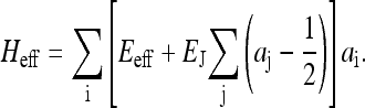
THE HYBRID MODEL FOR COLLECTIVE KINASE ACTIVITY

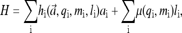
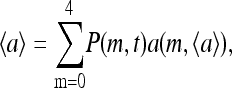
Our model describes the behavior of a cluster of N interacting receptors. The network of receptors does not have to be on a regular lattice, as long as a set of neighboring receptors is defined for each individual receptor in the network based on physical proximity. The properties of a receptor i, labeled by its receptor type q_i (Tar, Tsr, Tap, etc.), can be described by three dynamic variables: m_i ∈ [0, 4] is its methylation state; l_i is its ligand binding status (l_i = 1 means the receptor is occupied by a ligand, and l_i = 0 means the receptor is vacant); a_i is its activity (a_i = 1 means the receptor is active, and a_i = 0 means the receptor is inactive). In our model, the receptor cooperativity is modeled by interaction between the receptor activities (a_i's). The overall normalized kinase activity of the whole system is simply characterized by the average of all individual receptor activities: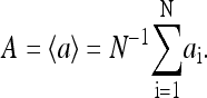

The timescales for the receptor activity change (τ_a) and ligand binding/unbinding process (τ_l) are much faster than that of the methylation/demethylation processes (τ_m). Since we are mostly interested in behaviors of the system at a timescale (τ) larger than τ_a and τ_l, but smaller than τ_m (τ_l, τ_a ≪ τ ≪ τ_m), the kinetics of the system can be conveniently described by a hybrid model consisting of a quasi-equilibrium model of {a_i, l_i} for fixed methylation levels (m_i's) and the slow dynamics of {m_i} affected by the averaged activity of each receptor. Furthermore, the equilibration of a_i's and l_i's for a given set of m_i's may be described by an energy function (Hamiltonian), which can be considered as a simplification for the general rate-based kinetics used in our previous study (Mello and Tu, 2003b).

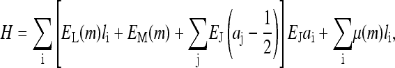
The activity of a receptor should depend both on its own properties (its methylation level and ligand binding status) and also on its neighbors' activities due to receptor interaction. A general form of the Hamiltonian governing the variations of the fast variables a_i and l_i for a given m_i can be written as

(1)

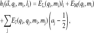
where refers to the activities of all the receptors. h_i is the activation energy, i.e., energy difference between the active and inactive configuration, for vacant receptors (when l_i = 0); and μ_i is the occupation energy, i.e., energy difference between the vacant and bound configuration, for inactive receptors (when a_i = 0).

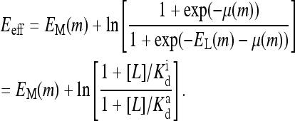
h_i has contributions from ligand binding, the methylation level of the receptor itself, and coupling to its neighboring receptors, parameterized by E_L, E_M, and E_J, respectively, in the following expression:

(2)

with j representing all the neighboring receptors of receptor i. E_M(m) is a decreasing function of methylation level m. E_L couples ligand binding l_i with receptor activity a_i. For attractants, E_L > 0 because ligand binding decreases kinase activity. The local (coupling energy excluded) activation energies are E₀(m) ≡ E_M(m) and E₁(m) ≡ E_M(m) + E_L(m) for vacant and ligand-occupied receptors respectively. “Ferromagnetic” coupling (i.e., E_J < 0) is used because receptor coupling is assumed to align activities of neighboring receptors.

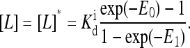
μ is essentially the chemical potential for inactive receptors to bind ligand. μ depends on the external ligand concentration and can be explicitly written as

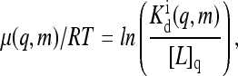(3)

where is the ligand dissociation constant for inactive receptors and [L]_q is the concentration of type q ligand that binds to type q receptor. (Here the Hamiltonian assumes each type of receptor binds to only one type of ligand; however, it is easy to generalize to include multiple ligand types.) RT is the thermal energy unit, which we set to be 1 from now on. For the active receptors, i.e., a_i = 1, the corresponding ligand dissociation constant can be easily obtained from the Hamiltonian (Eqs. 1 and 2):

(4)

The above relation between the ratio of the dissociation constants for active and inactive receptors and E_L is a direct consequence of energy balance in a Hamiltonian system. The only difference between our previous model (Mello and Tu, 2003b) and the model used in this article is that the relation of Eq. 4 was not enforced in Mello and Tu (2003b).

The receptor coupling strength, E_J, could in principle depend on the methylation levels of the interacting receptors. For simplicity, we omit such dependence for the rest of the article. In a true Hamiltonian model, the coupling constant should be symmetric under permutation of the receptor types, i.e., E_J(q_i, q_j) = E_J(q_j, q_i). However, there are no direct biological constraints enforcing such symmetry. In the case of asymmetric coupling strength, the energy function can be used only for each individual receptor to determine the transition rate between active and inactive conformations of the receptor while its environment, i.e., the activities of the neighboring receptors, is kept fixed.

In a recent work by Shimizu et al. (2003), a similar model was used but with several significant simplifications made for the Hamiltonian. First, only one receptor species was considered in their studies. Second, E_M was made to have the following simple form:

(5)

where E_m = −1.95 in the above equation is a constant, δ(m − 4) is only nonzero (equals to 1) when m = 4. Third, E_L(m) was made to be independent of m, in particular, it was set equal to −E_m. Last, the ligand binding constant was also made to be independent of methylation level m. Because E_L was a constant in their model, was therefore also independent of m through the relation in Eq. 4. In our study, we use this specific set of parameters as a reference point in the full parameter space to study the general properties of our model.

To complete the description of the system, we need to model the dynamics of the methylation level for each receptor m_i. In its simplest form, the slow methylation kinetics can be described by the methylation rate T_R(m_i, a_i) (from state m_i to state (m_i + 1)), and the demethylation rate T_B(m_i, a_i) (from state m_i to state (m_i − 1)). The StochSim approach (Morton-Firth et al., 1999) used in Shimizu et al. (2003) effectively calculated these rates by simulating all the detailed enzymatic reactions stochastically (although assuming that enzyme concentration was uniform throughout the cell). However, for understanding the behavior of the system, the most important feature of these transition rates is their dependence on the kinase activity of the receptor complex. A key property of these enzymatic reactions, inferred from the system's perfect (or near perfect) adaptability, is that these rates may depend on the activity (Barkai and Leibler, 1997; Yi et al., 2000; Mello and Tu, 2003a). The simplest way to achieve perfect adaptation is to let methylation take place only for the inactive receptors and demethylation take place only for the active receptors. This assumption can be expressed as

(6)

where k_R and k_B are rate constants, with the corresponding timescales τ_R = 1/k_R and τ_B = 1/k_B much longer than the equilibration time τ₀ = max(τ_a, τ_ℓ) of a_i and l_i.

Overall, for a given methylation configuration {m_i}, the quasi-equilibrium behavior of the {a_i, l_i} variables is governed by the Hamiltonian given in Eqs. 1 and 2. The averaged activity of the receptors in turn determines the slower kinetics of the methylation levels as given in Eq. 6. In the rest of the article, we study this hybrid model that includes a quasi-equilibrium statistical model for describing the fast variables coupled with a stochastic dynamic model for studying the methylation/demethylation processes.

METHODS: MEAN-FIELD THEORY AND MONTE CARLO SIMULATION

The above hybrid model does not have a known analytical solution, so the exact behavior of the model has to be studied numerically by Monte Carlo simulation. However, most of the behavior can be studied analytically by using mean-field approximations. We describe the details of the mean-field theory and the Monte Carlo simulation in this section.

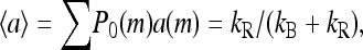
The mean-field theory

In the mean-field theory (MFT) approximation, each receptor interacts with a mean field 〈a〉 instead of with its specific neighbors. It can be formally described as a variation of the original Hamiltonian by allowing all receptors to interact with each other, i.e., the sum over j in Eq. 2 is now over all the receptors in the system. The interaction strength has to be normalized accordingly to preserve the total interaction strength: E_J is replaced by j₀E_J/N, where j₀ is the number of nearest neighbors of each receptor in the original model (e.g., j₀ = 4 for a square lattice) and N is the total number of receptors in the system. The mean-field Hamiltonian is then

(7)

where the mean field

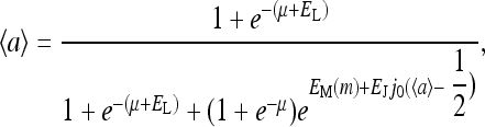
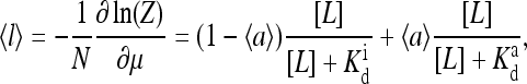
The mean-field system can be solved analytically because its Hamiltonian is just a sum of decoupled local terms. The average activity for site i depends only on its methylation level m (we have dropped the subscript i because of the spatially decoupled nature of the equations) and can be written as

(8)

The mean field 〈a〉 can be obtained by the self-consistency condition:

(9)

where P(m, t) is the fraction of receptors with methylation level m at time t. P(m, t) is simply governed by the flow equation in the m space:

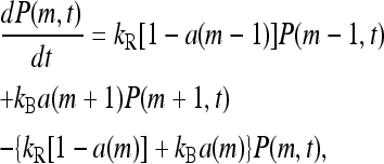(10)

for m = 0, 1, 2, 3, 4, and with the boundary conditions P(−1, t) = P(5, t) = 0 and the conservation condition

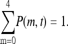(11)

Equations 8–11 determine the mean-field dynamics of the system.

A simplified mean-field theory

To understand the qualitative properties of the model, such as the existence and the characteristics of different steady states (phases), it is desirable to have the simplest mathematical theory that captures the essence of the dynamics. The mean-field theory described in the last section can be further simplified under the approximation that the methylation level m_i is a continuum variable, instead of being discrete. It is known that chemoreceptors form homodimers. Given the large number of possible combinatorial methylation states for the receptor dimer (2⁸ = 256), this approximation may not be unreasonable.

For the mean-field theory under the assumption of a continuum methylation level m, the dynamical equations for the methylation (Eq. 10) are simplified significantly to just one equation governing the dynamics of the mean methylation level m(t):

(12)

together with the activity equation

(13)

these two coupled equations determine the behavior of the simplified MFT.

Monte Carlo simulations

We have also explored the properties of our hybrid model using Monte Carlo (MC) simulations. Simulations were conducted as follows. The receptors filled a two-dimensional square lattice, typically of size N = 65 × 65 receptors. When multiple receptor types were used, the receptors were arranged randomly. Initial conditions were generally for the receptors to have methylation level m = 2, no bound ligand (l = 0), and activity of each receptor selected randomly to be 0 or 1. We are not concerned with the absolute timescale in this study; for convenience, the unit in time is set by the slow methylation timescale τ_R = 1/k_R. The system was evolved in time with random sequential updating. During Monte Carlo step of length Δt = 0.005, N receptors were selected at random, in sequence, to be updated. Updating of a receptor consisted of two steps: equilibration of the activity and ligand binding according to the energy function for a single receptor, and potential methylation or demethylation governed by the kinetic equations. For equilibration, for a given single receptor i, the energies E_i(a_i, l_i|m_i) for the four possible states a_i={0,1}, l_i={0,1} were computed. One of the four states, (a_i,l_i), was selected randomly according to the probability (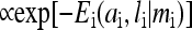). Based on the resulting a_i, the appropriate rate T_R or T_B was computed, and the probability for methylation (demethylation) to occur in this time step was T_RΔt (T_BΔt). A random number was generated, and methylation (demethylation) was performed if the random number was less than the probability.

RESULTS

Using the methods described above, we studied both steady-state (long time) and transient (short time) properties of the model for different stimuli. Many interesting observations on the response and the steady-state behavior of the system have been made in the recent study by Shimizu et al. (2003) using a similar but simplified model. Our emphasis here is to understand the underlying mechanisms of the observed phenomena for the more general model. We have also studied the behavior of our model in the absence of methylation dynamics, which is crucial in understanding many experiments with mutant strains and almost all of the in vitro experiments.

The steady-state behavior: phases and phase transition

At steady state, the fluxes of receptor populations in the m space have to be balanced, and we can replace Eq. 10 by its steady-state equation

(14)

for m = 0, 1, 2, 3, where P₀ is the steady-state probability. By summing the above equation over m, it is easy to see that the average steady-state activity of the system 〈a〉 will be a constant independent of ligand concentration

(15)

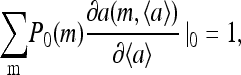
provided the following conditions are both satisfied:

(16)

These conditions can be strictly enforced by having E_M(0) = ∞ and E_M(4) = −∞ (i.e., a(0) = 1 − a(4) = 0), which leads to perfect adaptation, or by having large enough E_M(0) and −E_M(4), together with small receptor populations at m = 0 and m = 4 (i.e., a(0), 1−a(4), P₀(0), P₀(4)=1), which lead to near perfect adaptation.

Therefore, for a model with (near) perfect adaptation, the steady-state activity is given by the balance of the methylation and demethylation rates, independent of the ligand concentration. Essentially, the system adjusts its overall methylation level to regulate the activity of the system to be at exactly the desired level. However, this desired activity level is not always available to the system. Imagine the extreme situation in which the coupling constant is much larger than other energy scales in our model. Then the receptors of the system would be either all active or all inactive depending on the overall methylation level and ligand concentration. In this case, except for average activities near 0 or 1, the intermediate activity levels cannot be achieved in a steady-state solution of the model. As a result, in trying to reach an unavailable activity level, the methylation and demethylation processes drive the system into an oscillatory state between the fully active state and the fully suppressed state.

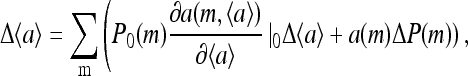
The simplest way to show the existence of the oscillatory phase in our model is by studying the mean-field theory. In particular, the results from the simplified MFT with continuum methylation levels are especially intuitive. In Fig. 1, we plot the MFT relation between the mean activity and the mean methylation (Eq. 13), together with the null line of the methylation kinetics Eq. 12, which is simply 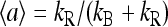in our model. The intersection of the two lines, which we call (m₀, a₀), is the fixed point of the system. The stability of the fixed point is determined by the sign of the local derivative 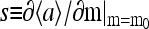for the activity versus methylation curve. For coupling strength |E_J| smaller than a critical value s is positive and it is easy to show that the steady-state fixed point is stable (Fig. 1 a). However, for larger values of |E_J|, the MFT relation between 〈a〉 and m is no longer monotonic and there are multiple solutions of 〈a〉 for a given m for a range of m and 〈a〉. When the fixed point activity a₀ falls within this activity range, s is negative and the fixed point becomes unstable. The behavior of the model is then a limit cycle alternating between the two stable branches of the MFT line, as shown in Fig. 1 b.

FIGURE 1.

Illustration of the two different phases: (a) the stationary phase at and (b) the oscillatory phase at The activity-methylation relation is represented by the thick line. The horizontal thin line is the null line for the methylation kinetics: points below it will move toward higher methylation regions (toward the right along the thick line), and points above it will move to lower methylation regions (toward the left along the thick line). The slope of the activity-methylation relation at the intersection of the two lines determines the stability of the fixed point (•).

The existence of the oscillatory phase is a general result of frustration between the methylation dynamics, which drives the system toward a specific activity, and the high coupling constant, which makes the system (energetically) unstable at that particular activity level. The onset of the transition occurs when the derivative This transition is related to the phase transition in equilibrium Ising-like models, but the oscillation is due to the additional feature of our model introduced by the (nonequilibrium) methylation/demethylation dynamics. Quantitatively, the onset of the oscillatory phase occurs at a critical coupling constant larger than that of the Ising transition.

The different phases of the model were also investigated by simulating the complete hybrid model using the Monte Carlo method. In particular, the phase diagram was determined in detail for the energy parameters used in Shimizu et al. (2003), but using our simplified methylation kinetic equations with k_R = 1 and k_B = 1. E_J values from 0 to −5 were studied. The simulation was run for 100 time units to ensure that steady state was reached and then for an additional 657 time units to collect data. Values of the average activity over all receptors, 〈a〉, were recorded every 0.01 time unit (time step Δt = 0.005). The variance and the power spectrum of the average activity were also computed.

Two types of behavior, a nonoscillatory phase at weaker coupling and an oscillatory phase at stronger coupling, can be easily identified from the time series of average activity and their corresponding power spectrum, as shown in Fig. 2, a and b, respectively. To characterize the transition, the time variance of the spatially averaged activity can be calculated for any given ligand concentration [L]. As shown in Fig. 2 c for increased as the coupling strength increased (i.e., as E_J became more negative). We approximately associated the transition point with the maximum in the second derivative of variance versus E_J relation. The critical coupling had only a weak dependence on μ and thus on the concentration of ligand in the system, as shown in the inset of Fig. 2 c.

FIGURE 2.

Monte Carlo simulation of the system using energy parameters from reference Shimizu et al. (2003) (E_M(m) = (m − 2)E_m + δ(m − 4)E_m with E_L = − E_m = 1.95 and independent of m): (a) The average activity time series for steady-state (E_J = −2.5) and oscillatory (E_J = −4.0) phases. (b) The power spectrum (log plot) for the data shown in a. (c) The variance of the average activity versus the coupling constant; the transition point is defined as the coupling constant where this curve has the largest second derivative. “Phase diagram” in the (E_J, [L]) space is shown in the inset.

Even though the existence of oscillatory phase is quite evident in our simulation with finite number of receptors, we do not expect the oscillatory phase to persist in the thermodynamic limit of infinite system size. Although small systems can oscillate as a single unit, with all receptors approximately in phase with each other, we expect the phase coherence of such oscillation to decrease as the size of the system increases. The decoherence of the phase is based on very general symmetry arguments and should therefore restore the time translation invariance, i.e., the steady state of the system, in the infinite system (thermodynamic) limit (Grinstein and Tang, 1995). We simulated a range of system sizes (in the absence of ligand, with E_J = −4) from 32 × 32 to 260 × 260. We found that the variance in the average activity decreased significantly as the system size increased, indicating a decrease in the amplitude of the activity oscillations. Results are shown in Fig. 3.

FIGURE 3.

Power spectrum (semilog plot) of the average activity time series for different system sizes with E_J = −4.0 and other parameters the same as in Fig. 2. Variance of the average activity over time versus system width is shown in the inset. The decoherence of the oscillatory phase for larger systems is evident as the variance decreases rapidly with an apparent stretched exponential decay with the fit of 0.25 exp(−0.1w^0.64), where w is the system width.

The correlations between different receptors as a function of their separation d were also studied. Not surprisingly, the activity correlation C_a(d) increased with stronger coupling constants. We also found that the methylation correlation (with the distance between the two receptors i and j equal to d) showed observable anticorrelation of up to −0.2 for adjacent receptors (d = 1) but was ∼0 for longer distances.

For independent receptors, the difference in their methylation levels leads to the difference in their activity, which in turn evens out the methylation level difference because of the way methylation rates depend on activity. For interacting receptors, the coupling between neighboring receptors decreases their activity difference and therefore weakens the restoring force for methylation level difference. This is the main reason for the observed small anticorrelation in methylation levels of neighboring receptors. This anticorrelation can be understood more systematically in a modified mean-field theory, which takes into account nearest neighbor receptor correlations. The modified mean-field theory is presented in the Appendix of this article.

Of the two types of behavior (phases) we found in our model, the oscillatory phase has yet to be observed experimentally, so we leave the discussion on possible experimental verification to the end of the article. In the rest of the results section, we confine our model to the parameter space corresponding to the nonoscillatory phase and study its relation to various existing experiments.

Enhanced gain in response to step function stimulus

Even though chemotaxis is the behavior of cells in following a spatial chemical gradient, it is achieved in bacteria by temporal sensing (Segall et al., 1986). Therefore, the majority of the experimental studies on bacterial chemotaxis can be conveniently carried out by subjecting the cell to a pure temporal stimulus, i.e., a step function change of the chemoattractant (or repellent) concentration in time. Due to the separation in timescales for ligand binding (τ_ℓ), receptor conformational change (τ_a) and the methylation/demethylation processes (τ_m), the response can be separated into the initial (fast) response to the stimulus, and the longer time relaxation, when methylation and demethylation play important roles. The short time response is a measure of the sensitivity of the system, which is the focus of this subsection.

For a given ambient external ligand concentration ([L]₀) represented by a constant “chemical potential” 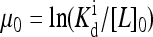in our model, the equilibrium state of the system can be described by the steady-state distribution of receptors in different methylation states, P₀(m). Upon a sudden change of external ligand concentration (Δ[L]), the chemical potential changes from μ₀ to μ = μ₀ + Δμ, with 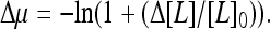For the short time response, the methylation levels of receptors have no time to adjust. The short time activity change (immediate response) can therefore be determined by the Hamiltonian (Eq. 1) with the fixed prestimulus receptor methylation distribution P₀(m), but for a new chemical potential μ₀ + Δμ.

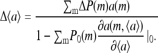
For realistic environments, the change in external ligand concentration is usually small, and linear response calculations are often useful. Using the mean-field theory approach, for small changes Δμ, we can compute the linear response by expanding Eq. 9 at t = 0⁺:

(17)

from which we obtain the linear response:

(18)

The subscript 0 here and afterward in the derivatives means the derivatives are taken at the prestimulus values of parameters, e.g., at μ = μ₀. At larger coupling strength |E_J|, the activity is influenced more by the average activity of its neighbors (as is evident from Eq. 8), and therefore is larger, leading to an increased linear response Δ〈a〉 diverges when the denominator in Eq. 18 goes to 0, i.e., when

(19)

which determines the transition point between the oscillatory-nonoscillatory phases for the mean-field model. The critical surface is given by

(20)

We also studied the response of the system to arbitrary increases in ligand concentration by simulating the full model, mostly for the reference energy parameters used by Shimizu et al. (2003). These simulations were done with different coupling strengths and for various initial ambient concentrations of ligand.

In Fig. 4 a, we plot the response activity versus the change in ligand concentration for several different initial concentrations for E_J = −2.5. When the response curves were shifted by subtracting the minimum activity and rescaled to range between 0 and 1, they were well fit by a Hill equation with Hill coefficient ∼1. The fit curves are also shown in Fig. 4 a.

FIGURE 4.

(a) Response curve (to a step change in ligand concentration) for the wild-type cell (with one receptor species) with the same parameters as in Fig. 2, and E_J = −2.5. Different symbols correspond to different ambient ligand concentrations (specified in the legend in units of ). After subtracting the minimum activity and scaling the activity to between 0 and 1, each data set is fitted by Hill function. The rescaled Hill functions are plotted as curves. All the fitted Hill coefficients are ∼1. (b) Sensitivity of the system, defined for doubling of the ligand concentration, plotted versus the ambient ligand concentration in units of for different values of coupling strength E_J = 0, −1.25, and −2.5.

Technically, gain of the signaling pathway (i.e., before the signal affects the motor) is defined as the ratio between fractional kinase activity change and the change in receptor occupancy. However, experimentally, it is difficult to measure receptor occupancy directly; therefore, the strength of the response is often more conveniently characterized by the sensitivity of the system, defined as the ratio between fractional activity change and the fractional change in ligand concentration. It is easy to see from the definitions that the gain and sensitivity are closely related to each other, and they are both good characterizations of the signal amplification in the system (Sourjik and Berg, 2002b; Mello and Tu, 2003b). Two such measures of sensitivity were considered in this article. The first was the normalized susceptibility,

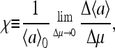(21)

where is the prestimulus activity. χ was computed numerically by fitting the versus Δμ curve by a quartic polynomial passing through the origin and using the coefficient of the linear term. The second measure was the fractional change in activity in response to a doubling of ligand concentration (Δμ = −ln 2), divided by Δμ, as used in Shimizu et al. (2003).

As expected, the sensitivity by both measures was maximal within the same range of μ₀ but declined for very large and very small μ₀. The μ₀ range for significant sensitivity corresponded to ∼2 orders of magnitude in ligand concentration, as shown in Fig. 4 b. In comparison, the sensitivity for a system without receptor coupling is ∼1 order of magnitude smaller. The sensitivity due to doubling the ligand concentration was smaller (within 50%) than that computed from the susceptibility, because doubling the ligand concentration was beyond the range of linear response. We note that the sensitivity from doubling the ligand concentration was numerically a more robust measure of amplification because the estimated susceptibility was sensitive to noise for small Δμ.

The response curves due to change in ligand concentration for E_J = −3.1 were similar to those seen for E_J = −2.5 (data not shown). They were associated with slightly larger sensitivity. When the activity was rescaled to range from 0 to 1, the response curves could be fit by a Hill equation but less closely because of noise in the response to small Δμ. A coupling strength stronger than the critical coupling, i.e., in the oscillatory phase, was also tried (E_J = −4), but the response was very noisy, particularly for small Δμ, so that a smooth response curve could not be generated even for larger numbers of runs.

The heightened signal gain in the model confirms the importance of receptor coupling. However, quantitatively, with the reference model parameters, the range of ambient ligand concentrations over which high sensitivity exists is only ∼2 orders of magnitude, short of the four decades observed experimentally (Sourjik and Berg, 2002b). The extremely broad range of high sensitivity may be explained if is made to depend on methylation, as assumed in our previous study (Mello and Tu, 2003b). The dependence of on methylation was also concluded from modeling of in vitro response data by Bornhorst and Falke (2003). In terms of the detailed behaviors of the response curves, the current model with the reference parameters does not match the experiments either. In particular, the activity did not approach zero when a saturating concentration of ligand was added in the reference model. This problem arose because with the reference energy parameters, the activity of receptors with methylation state m = 3, 4 was fairly large, even when bound with ligand. The problem may be remedied by increasing E_L for larger m, i.e., to make E_L dependent on the methylation level. These quantitative observations suggested that the energy form used by Shimizu et al. (2003) may be oversimplified. We expect that both E_L and should depend on methylation level m.

Overshoot in response to a strong pulse stimulus

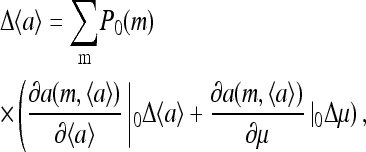
Another important type of temporal stimulus is a large change of the ligand concentration for a short period of time Δt, i.e., a pulse. During a strong pulse of attractant, the kinase activity of the cell is highly suppressed, and in the meantime the overall methylation level also increases by a small amount Δm ∝ k_RΔt. However, the effect of this small methylation level change on the activity can be amplified due to receptor coupling. As a result, instead of relaxing monotonically back to its prestimulus level after the pulse, the activity can overshoot to a higher value (than the prestimulus activity) before it finally relaxes back to the prestimulus level. This “overshoot” phenomenon was first observed experimentally for strong pulses (Block et al., 1982; Segall et al., 1986). Using mean-field theory, we can show in the following that the existence of the observed overshoot is directly related to the signal amplification as discussed in the last subsection.

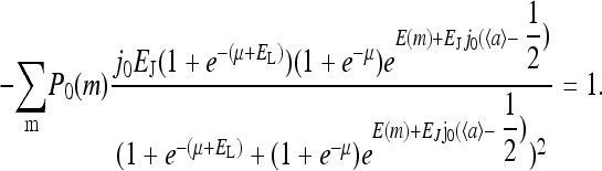
At the end of the pulse, the ligand concentration returns to its prestimulus level, but the system is left with a small change in the receptor methylation level distribution: The resulting change in activity (from the prestimulus level) can be determined approximately in the mean-field theory by the linear expansion of the self-consistent Eq. 9:

(22)

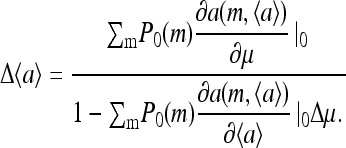
from which the activity change can be expressed as:

(23)

The numerator in the above expression represents the direct consequence of the stimulus; it is proportional to the small methylation change caused by the pulse. However, the overall activity change is amplified if the denominator 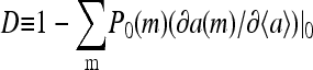is small also. In fact, the same denominator appears in the expression for signal amplification (Eq. 18). For large receptor coupling approaching D is found to be small, approaching 0. Therefore, due to the same mechanism of receptor coupling, a small change in methylation level distribution caused by a strong but short pulse can cause a significant overcorrection of the system's activity right after the strong pulse, and the activity relaxes back to its prestimulus level only when the overall methylation level returns to its prestimulus level over longer times.

We have studied the response to a pulse in ligand concentration using MC simulation with the parameters given in Shimizu et al. (2003). The system is first run for a long time with no ligand to equilibrate. At time t = 120, a high ligand concentration, characterized by μ = μ_p, is applied to the system for a short duration Δt before it is turned off. Time traces of the average activity, average methylation state, and average ligand occupancy were recorded from t = 100 to t = 130. For each set of conditions, time traces from 10 duplicate simulations were averaged to minimize noise. The coupling E_J = −2.5 was studied in the greatest detail, for μ_p between +1 and −3.5 and for pulse lengths Δt between 0.05 and 0.25. The pulse caused a sudden decrease in activity. The interval in which activity was lowered was defined from the time when the activity dropped below its prepulse average value to the time that it returned above this value. The activity overshot its initial value, and the overshoot interval was defined from the time the increasing activity surpassed its prepulse average to the time the activity decreased back to this average. The time integral of the deviation of the activity from its average was determined for both the initial response and for the overshoot.

The averaged time series of the activity and methylation levels for a strong pulse with saturating amount of ligand (μ_p = −3.5) with a short time period (Δt = 0.05) are shown in Fig. 5, a and b. The overshoot in activity is rather pronounced after the peak in average methylation level, and even a second peak in activity can be seen in Fig. 5 b. The individual activity relaxation rate is much faster than the methylation/demethylation rates; however, the global activity relaxation rate is affected by receptor coupling and can be lowered significantly at strong receptor coupling (i.e., analogous to critical slowing down in critical phenomena). Depending on the relative strength of the methylation/demethylation rates and global activity relaxation rate slowed by receptor coupling, the overall decay to the prestimulus activity level may have an oscillatory component, leading to the damped oscillation in Fig. 5, a and b. The duration and strength of the activity suppression and overshoot for different pulse durations are summarized in Fig. 5, c and d. Interestingly, even though the durations of the activity suppression and overshoot are quite different, the corresponding integrated strengths are always very close to each other.

FIGURE 5.

Response of the system: (a) average methylation and (b) average activity, to a short pulse (Δt = 0.05) with saturating strength (μ_p = −3.5). The response can be characterized by the durations of the immediate activity suppression and the subsequent overshoot, and the integrated strength of these two responses. These two measures of the response are plotted in c and d, respectively, for different pulse duration (with the same saturating strength μ_p = −3.5).

Behavior of the CheRCheB mutant strains (I): single type of receptors

The properties of each receptor, such as its kinase activity and binding affinity for ligand, may depend on the receptor's methylation level. However, it is difficult to obtain the methylation level dependence from measurements on WT cells because of the dynamical methylation and demethylation processes. To better understand the methylation dependence, it is therefore desirable to turn off the methylation/demethylation processes. Experimentally this is achieved by creating mutant strains of bacteria with the methylation enzyme CheR or the demethylation enzyme CheB or both knocked out. In this and the next subsection, we study the behavior of our model for such mutant strains, in which the methylation level of each receptor is fixed.

The simplest case, which we treat in this subsection, corresponds to the situation where there is only one type of receptor with a unique methylation level. Most of the in vitro experimental studies fall into this category. For this simple situation, the general energy function Eqs. 1 and 2 can be simplified:

(24)

where m is the unique and fixed methylation level of all the receptors. Since the dependence of the Hamiltonian on the receptor occupancy l_i is linear, l_i can be summed over easily in the partition function Z:

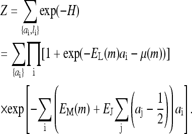(25)

For binary variable a_i = 0 or 1, using the identity where the partition function can be further simplified to

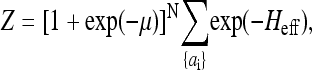(26)

where the effective Hamiltonian for the activity alone is

(27)

This is exactly the Ising model with an effective external field E_eff given by

(28)

The effective field E_eff depends on the ligand concentration [L], or equivalently on the chemical potential μ(m). For very high chemical potential, or when ligand concentration is much smaller than 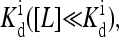the effective external field is approximately the same as the activation energy of the vacant receptors, E₀. For very low chemical potentials, or when ligand concentration is much larger than 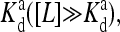the effective external field is approximately the activation energy of the occupied receptors, E₁. For ligand concentrations in between, i.e., 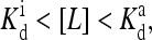the effective field interpolates between these two extreme energy values. We depict the dependence of the external field E_eff on the external ligand concentration schematically in Fig. 6. This reduced model for CheRCheB mutant is similar to one studied by Shi and Duke (1998). Our model naturally includes multiple levels of methylation as compared to the single methylation level model of Shi and Duke, and the derivation of this Ising-like model from a more general model makes our model easier to compare with experiments.

FIGURE 6.

Behavior of a mutant strain with a single methylation level can be mapped to an Ising model exactly. The dependence of the effective external field in the reduced Ising model is shown schematically as a function of the chemical potential 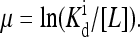At low ligand concentrations below the dissociation constant of the inactive receptor the external field is essentially equal to the activation energy of the vacant receptor: E_eff ∼ E₀(≡ E_M). At high ligand concentrations above the dissociation constant of the active receptor the external field is essentially equal to the activation energy of the ligand occupied receptor: E_eff ∼ E₁(≡ E_M + E_L). In between and the external field interpolates between E₀ and E₁.

Much is known about Ising model, one of the best-studied models in statistical physics, and this knowledge can now be directly used to understand the behavior of our system. The behavior of the (two-dimensional) Ising model depends strongly on the coupling strength. For coupling strength below its critical value, the dependence of the total activity on the external field is monotonic and continuous, passing through at E_eff = 0. The slope of the response curve at E_eff = 0, a measure of cooperativity, increases indefinitely as the coupling constant approaches its critical value. For coupling constants larger than the critical value, the dependence of on E_eff becomes discontinuous at E_eff = 0, as a gap in opens up at E_eff = 0. Extra variation in the response behavior is introduced in our model by the dependence of the “external field” on the ligand concentration, parameterized by the methylation level dependent variables E₀ and E₁ and Experimentally, the detailed response curves of activity versus ligand concentration do show significant quantitative differences for different mutant strains and under different experimental conditions (Borkovich et al., 1992; Bornhorst and Falke, 2001; Li and Weis, 2000). Qualitatively, the diversity in the response behavior could be explained by the fact that different mutant strains have to be characterized by different parameters (E₀, E₁, and ), and different experimental conditions could also affect the coupling strength. The ultimate test for the model would be to explain quantitatively all the different experimental data within the same model; for that purpose, more controlled, quantitative experiments and better understanding of how experimental conditions, such as receptor concentrations, affect the coupling strength are needed.

The simplified mutant strain model with all the receptors at a fixed methylation level was studied also by Monte Carlo simulation to demonstrate the range of possible behaviors. For these mutant strain simulations, methylation and demethylation rates were set to 0, and all the behaviors were determined by the Hamiltonian.

Coupling between receptors was kept weaker than the Ising critical point. E_M(m) = (m − 2)E_m + δ(m − 4)E_m with E_m = −1.95, the same as in Shimizu et al. (2003), was used; however, we used E_L = 2.5 for m = 2 and E_L = 4 for m = 3 to ensure that the activity approached 0 at saturating ligand concentration. As can be seen from Fig. 7, increasing receptor coupling has drastically different effects on activity for systems with different methylation levels. The m = 2 system had activity 1/2 in the absence of ligand, but addition of even small amounts of ligand acted as an applied field to inactivate the receptors, and receptor coupling enhanced this inactivation. Therefore, the activities are suppressed by strong receptor coupling for systems with low methylation level, as shown in Fig. 7 a. The m = 3 system had activity > in the absence of ligand, so that the coupling worked to increase the activity until the ligand concentration caused the activity to fall below after which the coupling helped decrease the activity. Therefore, stronger coupling led to steeper response curves for systems with higher methylation level, as shown in Fig. 7 b.

FIGURE 7.

Average activity of the mutant strain at various receptor coupling strengths with different methylation levels: (a) m = 2 state, because E₀ = 0 and E₁ = 2.5 are both greater than or equal to zero, the inactivation by ligand binding is enhanced by receptor coupling; (b) m = 3 with E₀ = −1.95 and E₁ = 2.05, depending on the ligand concentration, the average activity spans over the full range between 0 and 1. The transition region becomes sharper as the coupling constant is increased.

Another important property of the system is the average receptor occupancy and are strongly correlated as receptor occupancy directly affects the receptor activity. They are not linearly related to each other, however, due to the interplay between receptor coupling and the effective local field. From the simplified partition function for our model, the relation between the average receptor occupancy and the average activity can be easily determined:

(29)

where the average activity can be formally expressed as 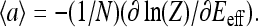The above relation between and is rather intuitive given that the active and inactive receptors have different ligand binding affinities.

For a given receptor type whose effective external fields are E₀ < 0 and E₁ > 0 for its vacant and ligand occupied states, respectively, we can study the relation between its ligand occupancy and activity. For convenience of comparison with the average activity we define the receptor vacancy rate 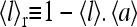and have the same trend for their dependence on the external ligand concentration [L]: they both decrease from 1 to 0 as [L] increases. However, depending on the values of E₀ and E₁, these two curves can be shifted from each other, i.e., their half maximum points occur at different ligand concentration values. The curve passes through the half activity point at E_eff = 0, which occurs at the ligand concentration

At the same ligand concentration, the receptor vacancy can be determined from Eq. 29:

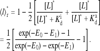(30)

From the above expression, at the half activity point, the receptor occupancy can be either close to 1 if and or close to 0 if and or close to 1/2 if E₀ + E₁ ≈ 0. The different types of behaviors for and versus [L] for different values of E₀ < 0 and E₁ > 0 are illustrated in Fig. 8 a. These results can also be explained rather intuitively from the occupancy half maximum point, where half of the receptors have a local field of E₁ and another half have a local field of E₀. In the presence of strong receptor coupling, the receptors with the larger absolute values of local field dominate, leading to the average activity to be either ≈ 0 (if ) or ≈ 1 (if ) at which leads to the separation of the two response curves.

FIGURE 8.

(a) Average activity (solid curves) and ligand occupancy (dashed curves) versus ligand concentration (in units of ) with E_J = −1.25, E_L = 4.0, and three different values of E_M (shown in the legend), corresponding to different values of (E₀, E₁): E₀ = −0.5, E₁ = 3.5 (•); E₀ = −2.0, E₁ = 2.0 (▪), and E₀ = −3.5, E₁ = 0.5 (♦). Notice the different relative relations of and for the three different cases, which roughly represent the general behaviors for low (•), medium (▪), and high (♦) methylation levels respectively. (b) The nonlinear relationship between and is shown for the three cases in a.

As shown directly in Fig. 8 b, the relation between occupancy and activity could be highly nonlinear. In general, for receptors with a low methylation level, the activities are lower due to larger E₁ and smaller |E₀|. Therefore, the activity curve will trail the occupancy curve. On the other hand, for a system with high methylation level receptors, where larger activity requires a large |E₀| and smaller E₁, the occupancy curve will trail the activity curve. This general behavior is consistent with the recent in vitro experiments by Levit and Stock (2002).

Behavior of the CheRCheB mutant strains (II): multiple receptor types

A more complicated situation is where there are two or more types of receptors, each type with a unique methylation level. Despite the existence of multiple receptor types, it can be shown that the same simplification of Hamiltonian as in the previous subsection can be carried out by summing over the ligand binding variable {l_i}. However, each receptor now has a local field, which is different for the different receptor species and/or different methylation levels, thus giving rise to an Ising-like model with heterogeneous local field. A related model studied in the physics literature is the so-called random field Ising model, where the local field is random with zero mean and a nonzero variance. For the random field Ising model, the system becomes ordered only at a much higher coupling constant than that of the homogeneous system, if at all. Intuitively, the random local field competes with the ferromagnetic coupling, and coherence over the whole system becomes harder to achieve. This argument is generally applicable for our model in the case of multiple receptor types. As a consequence, assuming the coupling constant to be the same, the response curve of the system with multiple receptor types is more gradual than that of the single receptor type system. This can be easily seen from the comparison of the response curve of the mutant with single methylation level (Fig. 7 b), which is already very steep at E_J = −1.5, and that of the model with receptors in different methylation states (Fig. 4 a), which is gradual even with a much larger coupling constant E_J = −2.5.

Besides the apparent cooperativity, the overall activity level of the multiple receptor type system can also be greatly affected by the receptor couplings. This is clearly demonstrated in the recent mutant studies by Sourjik and Berg (2002b), where CheR, CheB, or both are knocked out in the wild-type cells, and the response of the system to methyl-aspartate is studied in vivo by using fluorescence resonance energy transfer. For example, the activity changes for the same receptor, Tsr with m = 2, upon ligand occupation were found to be different in different CheRCheB mutant strains. This is one of the evidences suggesting the existence of strong coupling between Tar and Tsr. For this particular example mentioned here, since the Tar receptors in different CheRCheB mutant strains have different methylation levels, strong coupling between Tar and Tsr leads to different activity changes for Tsr. Indeed, incorporating such heterogeneous receptor coupling into a mean-field theory, we were able to fit the experimental data from all the six mutant strains simultaneously using the same set of parameters. The details and important implications of such a study can be found in our original article (Mello and Tu, 2003b). However, one concern is that MFT is just an approximation of the full model. In the following, we study the response behavior of the hybrid model using both the mean-field theory and the full Monte Carlo simulation. Our emphasis in this article is to explore the consistency between the mean-field theory and the full Monte Carlo simulation, in particular for the parameter regime where MFT shows good agreement with experiments.

Considering only the major chemoreceptor types Tsr and Tar (with abundance ratio Tsr/Tsr = 2:1), each mutant strain can be characterized by two methylation levels m_Tar (for Tar receptor) and m_Tsr (for Tsr receptors). The six mutant strains used in the SB experiments, CheR⁻, CheB⁻, CheRCheB(EEEE), CheRCheB(QEEE), CheRCheB(QEQE), and CheRCheB(QQQE), can therefore be conveniently represented as (m_Tar, m_Tsr) = (0, 0), (4,4), (0,2), (1,2), (2,2), and (3,2), respectively. In our model, each receptor has three independent parameters E₀(q, m), E₁(q, m) and (q, m), which depend on its species label q (q = 1 for Tar and q = 2 for Tsr) and methylation level m. The receptor interaction is described by four coupling constants E_J(q, q′) between the same and different chemoreceptor species. There are eight types of (major) chemoreceptors involved in SB's six mutant strains: five different Tar states (m = 0, 1, 2, 3, 4) and three different Tsr states (m = 0, 2, 4). For the MC simulation, the receptors were arranged randomly on a 65 × 65 square lattice, and the methylation/demethylation kinetics were turned off by setting k_R = k_B = 0. Response of these mutants to various ligand concentrations was determined by simulating them for 1 time unit to reach equilibrium and then an additional 15 time units to collect activity and ligand binding data.

Following the same approach as in our previous study (Mello and Tu, 2003b), we fit the results of the mean-field theory of our current model to the data from all the six mutant experiments to find the appropriate parameters for these eight types of receptors and the coupling constants. As in our previous study, we can fit our current MFT to all the mutant data accurately within the experimental error. Given the amount of data in each mutant experiment and the overlapping methylation states in the six different mutant strains, the fitting problem is highly nontrivial, and the fact that one can fit all the mutant data with a consistent set of parameters gives us confidence in the model itself. In fact, even with the large amount of mutant data and the simplicity of the model, there are many possible sets of parameters within our model that can be used to fit all six mutant experiments equally well. We took one such set of parameters, listed in Table 1, and simulated the full model using the Monte Carlo method to check the accuracy of the MFT in the parameter regime that is relevant for explaining the experiments. (The parameters are not unique. They can also be different from those used in our previous study (Mello and Tu, 2003b) because the model we used here is different.)

TABLE 1.

A set of parameter values that give a good fit between mean-field theory and the SB data for the six mutant strains

m	0	1	2	3	4
E0(1, m)	0.864	0.310	−0.147	−8.02	−20.1
E0(2, m)	4.69	–	−1.04	–	−7.97
E1(1, m)	30	2.10	1.41	0.763	0.740
E1(2, m)	30	–	30	–	30
(1, m)	2.43	21.3	18.0	0.0314	6.49 × 10−7
(1, m)	3.7 × 109	128.9	85.4	204.2	727.1
(2, m)	0.257	–	32539	–	24.9
(2, m)	2.5 × 1010	–	9.8 × 1017	–	7.7 × 1017
EJ(q,q′)		q′ = 1		q′ = 2
q = 1		0		−4.40
q = 2		−6.41		−1.38

The local parameters for each receptor type, E₀, E₁ (in unit of thermal energy) and (in unit of μM), are listed for each relevant receptor type characterized by (q, m), where q = 1 for Tar and q = 2 for Tsr, and m is the receptor methylation level. Values of (q, m) = exp(E₁ − E₀) are also included for reference; the effective dissociation constant is a complicated combination of and and it also depends on the actual activity. The coupling constants E_J(q, q′) (listed in the lower table) depend on the receptor species labels q and q′ for two neighboring receptors.

In Fig. 9, we plot the results from Monte Carlo simulation with the MFT parameters from Table 1 together with the experimental data from Sourjik and Berg (2002b). It is clear from Fig. 9 that the Monte Carlo results agree reasonably well with the experimental results, and hence do not differ significantly from the MFT results, which are fitted directly to the experimental results. We chose not to show the MFT results in Fig. 9 for clarity of the figure, with the understanding that the MFT results are mostly within a few percent of the experimental data. Interestingly, most of the discrepancy between the full MC model and the MFT occurs in the strain CheRCheB(EEEE). The detailed reason why this specific strain (CheRCheB(EEEE)) shows discrepancy is unclear, probably related to the fact that the same parameters for Tar(EEEE) are also needed to fit data for the CheR⁻ strain, which is the hardest to fit because of its extremely small activity and high sensitivity.

FIGURE 9.

Response curves of six different mutant strains with two receptor species, each in a different methylation state. We first fit the mean-field theory to the experimental data to obtain a set of parameters, for which the full Monte Carlo simulations were carried out. The resulting MC results, shown here as curves, agree with the experimental data, shown as symbols, reasonably well. This agreement also implies that the MFT is a good approximation for the full MC model for the parameters used in Table 1.

Technically, the consistency between the MFT and the full model provides us with a good fitting strategy for the full MC model. To fit the experimental data with the full MC model, we can first use the numerically more tractable MFT, and the resulting MFT parameters can serve as a good starting point in the parameter space for fitting the experimental data with the full MC simulation, which is much more computationally intensive.

Though it is not the purpose of this article to study the SB experimental data in detail (for that, see our previous article (Mello and Tu, 2003a)), an observation and some speculations are in order for an interesting feature found in the parameters listed in Table 1. There are many sets of parameters that can give rise to similar agreement between our model and the experimental data; the fact that we have the coupling constants E_J(1, 1) = 0 in Table 1 is purely fortuitous. However, we did find that in general the diagonal coupling constants, i.e., between the same type of receptor (Tar-Tar, Tsr-Tsr) are smaller than the off diagonal coupling constants, i.e., between Tar and Tsr. The reason could be that in the presence of both types of receptors, the direct interaction between Tar receptors is indeed small due to the way the heterogeneous receptor cluster is organized. Specifically, it could turn out that within the receptor cluster, the neighbors of any Tar receptor are mostly Tsr receptors. This hypothesis seems to be consistent with recent experimental works by Sandy Parkinson's lab (Ames et al., 2002; Ames and Parkinson, 2004), which showed preference of mixed team between Tar and Tsr within trimer of dimer receptor complex. However, in the absence of Tsr receptors, such as in the new experiments by Sourjik and Berg (2004), Tar receptors will have to team together among themselves, and the direct coupling between Tar and Tar could therefore be larger. Further work is needed to incorporate the new experimental results of Sourjik and Berg (2004) on mutants with one type of receptor and their earlier experimental data with both receptor types (Sourjik and Berg, 2002b) into a unified model.

Other effects, such as using a triangular lattice (in which receptors each have six nearest neighbors instead of four) for these mutants were also explored. The response curves for the triangular lattice were very close to those for the square lattice.

SUMMARY AND DISCUSSION

We proposed a model describing the kinase activity and adaptation process of the bacterial chemotaxis system. The model we constructed can be considered a general model that includes the important qualitative ingredients of the underlying biology: 1), the existence of multiple methylation levels for each receptor and their effects on kinase activity and ligand affinity; 2), interaction between the same and/or different types of neighboring chemoreceptors within the receptor cluster; 3), the possible effects of receptor conformation (activity) on the ligand binding affinity; and 4), the appropriate receptor methylation/demethylation dynamics that maintains high adaptation accuracy. In many aspects, our model is similar to previous models, especially the one studied recently by Shimizu et al. (2003). The uniqueness of our model lies in its generality; for example, we have included interactions between different types of receptors, and each receptor can have its own self-consistent activity and ligand binding parameters depending on its methylation level. The advantage of such a general approach is that we can study all experiments within the same model and at the same time different quantitative experiments can be fitted together to determine the model parameters.

In our model, the fast kinetics that describes the ligand binding and kinase activity of the receptors given their methylation levels is governed by an energy functional (Hamiltonian), whereas the slow process of receptor methylation/demethylation is described by kinetic rate equations. The simplification in describing the methylation kinetics makes the simulation of our model much faster than other stochastic models, such as the StochSim approach (Morton-Firth et al., 1999) used in Shimizu et al. (2003); this speedup is highly desirable for the numerically intensive task of parameter fitting. The properties of this hybrid model, which combines the (quasi)equilibrium description of the fast timescale and the dynamical equations describing the methylation process, were then studied in various regions of the parameter space and under external stimuli that are relevant for experimental observations. In particular, we focused on understanding the general consequences of receptor coupling.

Though adaptation happens at a much longer timescale, receptor coupling has a very interesting effect on the adaptation kinetics. We find that when receptor coupling strength increases, the model loses its ability to adapt. Instead, the activity oscillates around the preferred activity level. In our model, we can explain such oscillations analytically as an instability of the steady-state solution, caused by the strong coupling strength. As the coupling strength increases beyond a critical point, the equilibrium model of coupled receptor activities enters the symmetry broken phase, where there is a range of activity that is energetically unstable. This unstable activity range increases as the coupling strength increases. If the activity to which the system tries to adapt falls in this unstable range, the steady state with the preferred activity becomes unstable, and the activity instead oscillates between the two extremes of the activity gap.

The existence of the oscillatory phase is due to the interplay of perfect adaptation and strong receptor interaction and should be a general phenomenon independent of other details of the model. However, for a given cell, even if oscillations exist locally within the receptor cluster, the total activity variation will be damped by phase decoherence of such oscillations in different parts of the receptor cluster. Experimentally, for wild-type cells, the coupling constants may be well below the threshold for the oscillation, and any oscillation would be further eliminated or damped by measurements averaging over many independent individual cells. Therefore, any possible verification of the oscillatory phase would have to involve manipulating the coupling strength (e.g., by overexpressing the receptor complex proteins) and making single cell measurements. Other more specific, quantitative predictions based on our current model can only be made once the parameters of the model are determined.

It is generally accepted that receptor coupling could induce higher signal gain, as demonstrated here and in several previous studies (Bray et al., 1998; Duke and Bray, 1999; Shimizu et al., 2003; Mello and Tu, 2003b).

In addition, we find that the same mechanism for high signal gain in response to sustained ligand concentration change also seems to be responsible for the observed overshoot in the cell's response to a strong pulse. The pulse response study is very important in understanding the bacterial chemotaxis strategy (Segall et al., 1986).

A bacteria cell achieves chemotaxis by temporal comparison, i.e., comparing its present environment, characterized by the current ligand concentration, to its environment of the recent past, “memorized” by the receptor methylation level. The overshoot in pulse response can be therefore considered as the “memory” of a past event (a short pulse of ligand). Such memory persists for a few seconds for the cell to decide whether the situation has improved over that time period. As we can see here, receptor coupling not only amplifies the current signal, it also reinforces the memory so that the system can carry out the appropriate comparison and therefore make the correct decision.

The general concept of receptor coupling introduces another layer of complexity in modeling the bacterial chemotaxis process, i.e., different chemoreceptor species may interact with each other. Interaction between heterogeneous receptors was shown to be important in interpreting (Mello and Tu, 2003b) the recent in vivo response data (Sourjik and Berg, 2002b). The receptor coupling affects the overall activity and the sensitivity of each type of receptor involved. In general, heterogeneity, caused by either the existence of multiple types of receptor or multiple methylation levels of a given receptor type, reduced the Hill coefficient of the response curve. However, a low Hill coefficient in the response curve does not mean low gain because the gain is defined for small changes in external stimulus, far away from the steepest part of the response curve, where Hill function is most useful. In fact, as found in our previous study (Mello and Tu, 2003b), the signal amplification could come from receptors that are not directly bound to the ligand because of a large coupling between different types of receptors and the high sensitivity of these receptors maintained by the adaptation process. An important issue in bacterial chemotaxis is signal integration, i.e., how would the cell combine different sources of information represented by the presence of different chemoattractants (or repellents) in the medium (Khan et al., 1995; Adler and Tso, 1976)? The effects of heterogeneous receptor coupling on signal integration are expected to be extremely interesting (Gestwicki and Klessing, 2002).

Qualitatively, the inclusion of receptor coupling makes it easier to understand several key in vitro response experiments.

The different levels of cooperativity, often characterized by different Hill coefficients of the response curves (Bornhorst and Falke, 2001; Li and Weis, 2000), observed in different in vitro experiments, may be explained by their difference in receptor coupling strength. However, how receptor coupling strength depends on various protein concentrations (e.g., receptor CheW and CheA) and other parameters of the system remains a challenge.

Another important consequence of receptor coupling is the difference between receptor occupancy and the kinase activity. If the receptors are not coupled to each other, then receptor occupancy and activity indeed depend on each other linearly. However, if the coupling is strong enough, the activities of the occupied and the unoccupied receptor strongly affect each other, and depending on the relative activity (inactivity) of the unoccupied (occupied) receptors, the dependence of kinase activity on ligand concentration can be shifted away from that of the receptor occupancy, as observed experimentally (Levit and Stock, 2002). As a consequence, one should not use the receptor occupancy curve to infer activity, or vice versa.

Now that we have a general model that is capable of explaining various in vitro and in vivo experiments individually, the next step is to incorporate more and more high-quality quantitative data, from both the in vitro biochemistry type experiments and the in vivo experiments for different mutant strains and eventually wild-type cells, into a unified model with a consistent set of parameters. For many existing experiments, the data are consistent with the general properties of the model itself, and they impose important constraints for the parameters of the model. For example, from in vitro studies (Bornhorst and Falke, 2001; Li and Weis, 2000), we know that the activities of the system can always be suppressed to zero by saturation with ligand regardless of the methylation level. This observation sets constrains for the intrinsic energies of the model, i.e., E₁(m) > 0 for all m.

There are other cases where different experiments seem inconsistent with each other. For example, as reported in the in vitro experiments by Levit and Stock (2002), the receptor occupancy curves seems to be nearly independent of the methylation level of the receptor. However, in the recent in vivo experiments by Sourjik and Berg (2002b), the response curves of the wild-type cell seems to shift consistently toward larger ligand concentration with increasing ambient ligand concentration. This implies that for the receptors with higher methylation level, which are present in greater quantities at the high ambient ligand concentration, the ligand affinity is lower, i.e., larger dissociation constant K_d for larger m. As shown in our previous work (Mello and Tu, 2003b), the dependence of K_d on m together with adaptation is crucial for the system's high sensitivity over a large range of ambient ligand concentrations. Whether we can incorporate these findings from different experiments within the same model or whether we will need new ingredients for our model remains an interesting challenge.

APPENDIX: THE SECOND ORDER MEAN-FIELD THEORY

To study correlations between nearest neighbor receptors, we can introduce a second order mean-field theory that treats the nearest neighbor correlation explicitly. For this purpose, we define P(m, m′, t) as the joint distribution of a pair of neighboring receptors having methylation levels m and m′. To determine the dynamics of P(m, m′, t), we need to know the activity of a receptor with methylation level m and with one of its neighbors having methylation level m′, defined as a(m, m′). a(m, m′) can be written as

(31)

where with j = 1, 2, …, j₀ − 1 are the methylation levels of all the neighboring receptors except for m′ (j₀ = 4 for square lattice is used in this article). The conditional probability of a receptor in state m having a neighbor in state m′ is given by P(m|m′) = P(m, m′)/P(m′) with

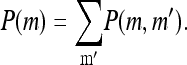
The above equation for all m ∈ [0, 4] and m′ ∈ [0, 4] and the dynamical equations governing the flow of P(m, m′, t) in the (m, m′) space determine the dynamics of the simplest second order MFT:

(32)

The main purpose of this more complicated MFT is to look for correlation in methylation levels between nearest neighbors, which was observed in our Monte Carlo simulations. This correlation has a simple intuitive explanation, but the MFT here provides us a quantitative measure of such correlation.

The effect of methylation correlation on the mean activity of a receptor is evident from Eq. 31. For a receptor with methylation m, if the methylation level m′ of its neighbor is increased, the activity a(m′, m) for that neighbor is higher, which results in an increase in the activity for the receptor with methylation level m through receptor coupling. The increased activity makes the receptor prone to lose methyl groups, i.e., decreasing m according to Eq. 10 leading to anticorrelation between m and m′.

Fig. 10 shows the time evolution of average methylation, activity, receptor occupancy, and methylation correlation between neighbors, defined as

(33)

The anticorrelation between neighbors emerges from an initially uncorrelated distribution, and its final value depends on the ligand concentration and the coupling constant. Fig. 11, a and b, show the overall methylation distribution of all the neighboring receptor pairs P(m₁, m₂) for the two extreme cases of zero and saturating ligand concentrations. In Fig. 11, c and d, the difference between the joint distribution P(m₁, m₂) and the product of the single site methylation distribution P(m₁)P(m₂) (as the joint distribution would be in a totally uncorrelated situation) are plotted. The anticorrelation is evident as the populations of the m₁ = m₂ states are smaller than it would be in the uncorrelated situation.

FIGURE 10.

Effect of adding a saturating amount of attractant at t = 20 to an initially depleted environment. The reference parameters (Shimizu et al., 2003) (see main text) are used, except for E_J = −1.5, a value close to the highest cooperativity that does not present oscillatory behavior. The initial receptor population is uncorrelated and has (see text for details).

FIGURE 11.

The joint distributions for methylation levels of two neighboring receptors P(m₁, m₂) for ligand concentrations: (a) [L] = 0 and (b) [L] = ∞. Difference between the joint distribution P(m₁, m₂) and the product of the single site methylation distribution P(m₁)P(m₂) for ligand concentrations: (c) [L] = 0 and (d) [L] = ∞. Notice the negative values for P(m₁, m₂) − P(m₁)P(m₂) along the diagonal line (m₁ = m₂), which indicates anticorrelation between m₁ and m₂.

References

- Adler, J. 1976. The sensing of chemical by bacteria. Sci. Am. 234:40–47. [DOI] [PubMed] [Google Scholar]
- Adler, J., and W. W. Tso. 1976. Decision-making in bacteria: chemotactic response of Escherichia coli to conflicting stimuli. Science. 184:1292–1294. [DOI] [PubMed] [Google Scholar]
- Alon, U., M. G. Surette, N. Barkai, and S. Leibler. 1999. Robustness in bacterial chemotaxis. Nature. 397:168–171. [DOI] [PubMed] [Google Scholar]
- Ames, P., and J. S. Parkinson. 2004. Crosslinking snapshots of bacterial chemoreceptor squads. Proc. Natl. Acad. Sci. USA. 101:2117–2122. [DOI] [PMC free article] [PubMed] [Google Scholar]
- Ames, P., C. A. Studdert, R. H. Reiser, and J. S. Parkinson. 2002. Collaborative signaling by mixed chemoreceptor teams in Escherichia coli. Proc. Natl. Acad. Sci. USA. 99:7060–7065. [DOI] [PMC free article] [PubMed] [Google Scholar]
- Barkai, N., and S. Leibler. 1997. Robustness in simple biochemical networks. Nature. 387:913–917. [DOI] [PubMed] [Google Scholar]
- Berg, H. C. 2000. Motile behavior of bacteria. Phys. Today. 53:24–29. [Google Scholar]
- Berg, H. C., and P. M. Tedesco. 1975. Transient response to chemotactic stimuli in Escherichia coli. Proc. Natl. Acad. Sci. USA. 72:3235–3239. [DOI] [PMC free article] [PubMed] [Google Scholar]
- Block, S. M., J. E. Segall, and H. C. Berg. 1982. Impulse responses in bacterial chemotaxis. Cell. 31:215–226. [DOI] [PubMed] [Google Scholar]
- Borkovich, K. A., L. A. Alex, and M. I. Simon. 1992. Attenuation of sensory receptor signaling by covalent modification. Proc. Natl. Acad. Sci. USA. 89:6756–6760. [DOI] [PMC free article] [PubMed] [Google Scholar]
- Bornhorst, J. A., and J. J. Falke. 2001. Evidence that both ligand binding and covalent adaptation drive a two-state equilibrium in the aspartate receptors signaling complex. J. Gen. Physiol. 118:693–710. [DOI] [PMC free article] [PubMed] [Google Scholar]
- Bornhorst, J. A., and J. J. Falke. 2003. Quantitative analysis of aspartate receptor signaling complex reveals that the homogeneous two-state model is inadequate: development of a heterogeneous two-state model. J. Mol. Biol. 326:1597–1614. [DOI] [PMC free article] [PubMed] [Google Scholar]
- Bren, A., and M. Eisenbach. 2000. How signal are heard during bacterial chemotaxis: protein-protein interactions in sensory signal propagation. J. Bacteriol. 182:6865–6873. [DOI] [PMC free article] [PubMed] [Google Scholar]
- Cluzel, P., M. Surette, and S. Leibler. 2000. An ultrasensitive bacterial motor revealed by monitoring signaling proteins in single cells. Science. 287:1652–1655. [DOI] [PubMed] [Google Scholar]
- Bray, D., M. D. Levin, and C. J. Morton-Firth. 1998. Receptors clustering as a cellular mechanism to control sensibility. Nature. 393:85–88. [DOI] [PubMed] [Google Scholar]
- Duke, T. A. J., and D. Bray. 1999. Heightened sensitivity of a lattice of membrane of receptors. Proc. Natl. Acad. Sci. USA. 96:10104–10108. [DOI] [PMC free article] [PubMed] [Google Scholar]
- Falke, J. J., and G. Hazelbauer. 2001. Transmembrane signaling in bacterial chemoreceptors. Trends Biochem. Sci. 26:257–265. [DOI] [PMC free article] [PubMed] [Google Scholar]
- Gestwicki, J. E., and L. L. Klessing. 2002. Inter-receptor communication through arrays of bacterial chemoreceptors. Nature. 415:81–84. [DOI] [PubMed] [Google Scholar]
- Grinstein, G., and L. H. Tang. 1995. Long-range correlations in systems with coherent (quasi)periodic oscillations. Phys. Rev. Lett. 74:912–915. [DOI] [PubMed] [Google Scholar]
- Khan, S., J. L. Spudich, J. A. McCray, and D. R. Trentham. 1995. Chemotatic signal integration in bacteria. Proc. Natl. Acad. Sci. USA. 92:9757–9761. [DOI] [PMC free article] [PubMed] [Google Scholar]
- Levit, M. N., and J. B. Stock. 2002. Receptor methylation controls the magnitude of stimulus-response coupling in bacterial chemotaxis. J. Biol. Chem. 277:36760–36765. [DOI] [PubMed] [Google Scholar]
- Li, G., and R. M. Weis. 2000. Covalent modification regulates ligand binding to receptor complexes in the chemosensory system of Escherichia coli. Cell. 100:357–365. [DOI] [PubMed] [Google Scholar]
- Maddock, J. R., and L. Shapiro. 1993. Polar location of the chemoreceptor complex in the Escherichia coli cell. Science. 259:1717–1723. [DOI] [PubMed] [Google Scholar]
- Mello, B. A., and Y. Tu. 2003a. Perfect and near perfect adaptation in a model of bacterial chemotaxis. Biophys. J. 84:2943–2956. [DOI] [PMC free article] [PubMed] [Google Scholar]
- Mello, B. A., and Y. Tu. 2003b. Quantitative modeling of sensitivity in bacterial chemotaxis: the role of coupling among different chemoreceptor species. Proc. Natl. Acad. Sci. USA. 100:8223–8228. [DOI] [PMC free article] [PubMed] [Google Scholar]
- Morton-Firth, C. J., T. S. Simizu, and D. Bray. 1999. A free-energy-based stochastic simulation of the tar receptor complex. J. Mol. Biol. 286:1059–1074. [DOI] [PubMed] [Google Scholar]
- Segall, J. E., S. M. Block, and H. C. Berg. 1986. Temporal comparisons in bacterial chemotaxis. Proc. Natl. Acad. Sci. USA. 83:8987–8991. [DOI] [PMC free article] [PubMed] [Google Scholar]
- Shi, Y. 2000. Adaptative Ising model and bacterial chemotatic receptor network. Europhys. Lett. 50:113–119. [Google Scholar]
- Shi, Y., and T. Duke. 1998. Cooperative model of bacterial sensing. Phys. Rev. E. 58:6399–6406. [Google Scholar]
- Shimizu, T. S., S. V. Aksenov, and D. Bray. 2003. A spatially extended stochastic model of the bacterial chemotaxis signalling pathway. J. Mol. Biol. 329:291–309. [DOI] [PubMed] [Google Scholar]
- Sourjik, V., and H. C. Berg. 2000. Localization of components of the chemotaxis machinery of Escherichia coli using fluorescent protein fusions. Mol. Microbiol. 37:740–751. [DOI] [PubMed] [Google Scholar]
- Sourjik, V., and H. C. Berg. 2002a. Binding of the Escherichia coli response regulator CheY to its target is measured in vivo by fluorescence resonance energy transfer. Proc. Natl. Acad. Sci. USA. 99:12669–12674. [DOI] [PMC free article] [PubMed] [Google Scholar]
- Sourjik, V., and H. C. Berg. 2002b. Receptors sensitivity in bacterial chemotaxis. Proc. Natl. Acad. Sci. USA. 99:123–127. [DOI] [PMC free article] [PubMed] [Google Scholar]
- Sourjik, V., and H. C. Berg. 2004. Functional interactions between receptors in bacterial chemotaxis. Nature. 428:437–441. [DOI] [PubMed] [Google Scholar]
- Yi, T.-M., Y. Huang, M. I. Simon, and J. Doyle. 2000. Robust perfect adaptation in bacterial chemotaxis through integral feedback control. Proc. Natl. Acad. Sci. USA. 97:4649–4653. [DOI] [PMC free article] [PubMed] [Google Scholar]