Field Theoretic Study of Bilayer Membrane Fusion. I. Hemifusion Mechanism

Abstract

Self-consistent field theory is used to determine structural and energetic properties of metastable intermediates and unstable transition states involved in the standard stalk mechanism of bilayer membrane fusion. A microscopic model of flexible amphiphilic chains dissolved in hydrophilic solvent is employed to describe these self-assembled structures. We find that the barrier to formation of the initial stalk is much smaller than previously estimated by phenomenological theories. Therefore its creation it is not the rate-limiting process. The relevant barrier is associated with the rather limited radial expansion of the stalk into a hemifusion diaphragm. It is strongly affected by the architecture of the amphiphile, decreasing as the effective spontaneous curvature of the amphiphile is made more negative. It is also reduced when the tension is increased. At high tension the fusion pore, created when a hole forms in the hemifusion diaphragm, expands without bound. At very low membrane tension, small fusion pores can be trapped in a flickering metastable state. Successful fusion is severely limited by the architecture of the lipids. If the effective spontaneous curvature is not sufficiently negative, fusion does not occur because metastable stalks, whose existence is a seemingly necessary prerequisite, do not form at all. However if the spontaneous curvature is too negative, stalks are so stable that fusion does not occur because the system is unstable either to a phase of stable radial stalks, or to an inverted-hexagonal phase induced by stable linear stalks. Our results on the architecture and tension needed for successful fusion are summarized in a phase diagram.

INTRODUCTION

The importance of membrane fusion in biological systems hardly needs to be emphasized. It plays a central role in trafficking within the cell, in the transport of materials out of the cell, as in synaptic vesicles, and in the release of endosome-enclosed external material into the cell, as in viral infection. Although proteins carry out many functions leading up to fusion, such as ensuring that a particular vesicle arrives at a particular location, or bringing membranes to be fused into close proximity, there is much evidence that they do not determine the actual fusion mechanism itself. Rather the lipids themselves are responsible for the evolution of the fusion process in which the lipid bilayers undergo topological change (Lee and Lentz, 1998; Zimmerberg and Chernomordik, 1999; Lentz et al., 2000).

The physical description of the fusion process has, until very recently, been carried out using phenomenological theories that describe the membrane in terms of its elastic moduli (Safran, 1994). The application of these theories to fusion has been reviewed recently (Zimmerberg and Chernomordik, 1999). The fusion path that has been considered by these methods is one in which local fluctuations are assumed to cause a rearrangement of lipids in the opposed cis leaflets, resulting in the formation of a stalk (Markin and Kozlov, 1983). To release tension imposed on the membranes by the reduction of the solvent between them, the inner cis layers recede, decreasing their area, and bringing the outer, trans, leaves into contact. In this way the stalk expands radially to form a hemifusion diaphragm. Creation of a hole in this diaphragm completes formation of the fusion pore.

In recent years, coarse-grained models of amphiphiles (Müller et al., 2003a) have been used to provide a microscopic, as opposed to phenomenological, description of membranes. Fusion was studied within two such models. One, in which nonflexible molecules were composed of three segments, was studied by Brownian dynamics simulation (Noguchi and Takasu, 2001); and the other, in which the amphiphiles were modeled as flexible polymer chains in solvent, was studied by Monte Carlo simulation (Müller et al., 2002b). Both models showed a markedly different path to fusion than the phenomenological approaches assumed. Along this new path, the creation of the stalk is followed by its non-axially symmetric growth, i.e., elongation. After the stalk appears, there is a great increase in the rate of creation of holes in either bilayer, and the holes are created near the stalk itself. After a hole forms in one bilayer, the stalk elongates further and surrounds it, forming a hemifusion diaphragm. Formation of a second hole in this diaphragm completes the fusion pore. Alternatively, the second hole in the other membrane can appear before the elongated stalk surrounds the first hole. In this case, the stalk aligns the two holes and surrounds them both forming the fusion pore. This mechanism has also been observed more recently in molecular dynamics simulations (Marrink and Mark, 2003; Stevens et al., 2003). As has been stressed by us recently (Müller et al., 2003b), this alternative mechanism can be distinguished experimentally from the earlier hemifusion mechanism because it predicts at least two phenomena that are not compatible with the earlier hypothesis. The first is lipid mixing between the cis leaf of one bilayer with the trans layer of the other, a phenomena that has been observed (Evans and Lentz, 2002; Lentz et al., 1997). The second is transient leakage through the holes, noted above, which is correlated in space and time with the fusion process. Just such correlated leakage has recently been observed and extensively studied (Frolov et al., 2003).

The Monte Carlo simulations of the fusion process showed very clearly the nature of the process, and obtained quantitative correlations between leakage and fusion. Unfortunately, simulations are computationally expensive, so that investigation of the fusion process for different molecular architectures and membrane tensions is impractical. Moreover, simulations are not well suited for calculating free energy barriers of the fusion intermediates in the mechanism observed over a wide range of tension and amphiphilic architecture. Not only would one like to obtain these barriers, one would also like to compare them to those of the intermediates involved in the original hemifusion mechanism. To do so, we employ a standard model of amphiphilic polymers, which we describe in the next section, and solve it within the framework of self-consistent field theory (SCFT). In the first article of this series we examine the original hemifusion mechanism, whereas in the second we shall consider the new mechanism observed in the simulations.

In Properties of Isolated Bilayers we present the basic properties of the isolated bilayers and monolayers that result from our calculation. These properties include the spatial distribution of hydrophilic/hydrophobic segments, the area compressibility, the bending rigidity, and spontaneous curvature. We compare them to those obtained independently from previous Monte Carlo simulations, and from experiments on liposomes and polymersomes. It should be noted that these effective macroscopic properties are calculated within our microscopic approach, and are not required as input, in contrast to the common phenomenological descriptions of fusion based on membrane elasticity theory.

In Energetics of the Stalk and of its Radial Expansion we examine the free energy landscape along the standard hemifusion pathway, the path shown in Figs. 1 and 2. This is the same path assumed in phenomenological approaches, but we use a microscopic molecular model to calculate the distribution of microscopic components in the system along this trajectory, and the free energy that results. The initial configuration of the system is that of two parallel bilayers (Fig. 1 a). Hydrophilic portions of the amphiphile are shown as dark shaded, hydrophobic portions are shown as light shaded, and solvent is shown as unshaded. To bring the bilayers into close contact requires energy to reduce the amount of solvent between them. Consequently the free energy per unit area, or tension, of the bilayers increases. Fusion is one possible response of the system to this increased tension. Along the standard pathway, close contact of the cis layers is followed by the creation of an axially symmetric unstable intermediate, or transition state, shown in cross section in Fig. 1 b, which leads, under conditions detailed below, to a metastable, axially symmetric stalk, Fig. 1 c. If the system is under sufficient tension, this stalk pinches down, passes through another unstable intermediate (Fig. 1 d), and expands to form a hemifusion diaphragm (Fig. 1 e). To determine the radius at which a hole forms in this diaphragm to complete the fusion pore, we calculate in Formation and Expansion of Fusion Pore the free energy of an axially symmetric fusion pore as a function of its radius. Density profiles of fusion pores are shown in Fig. 2. We assume that when the free energy of the expanding hemifusion diaphragm exceeds that of a fusion pore of the same radius, a hole forms in the diaphragm converting it into a fusion pore (Fig. 2 b). Not surprisingly, the radius of the fusion pore that is formed cannot be too small, as in Fig. 2 a, for then its free energy would be higher than that of the hemifusion diaphragm. Once the pore has formed, it will expand if the membranes are under tension. Fig. 2 c shows the profile of an expanded pore, although this one is in a membrane of zero tension. We are able to calculate the free energy of the system at all stages of the pathway for various architectures of the amphiphile and tensions of the membrane.

FIGURE 1.

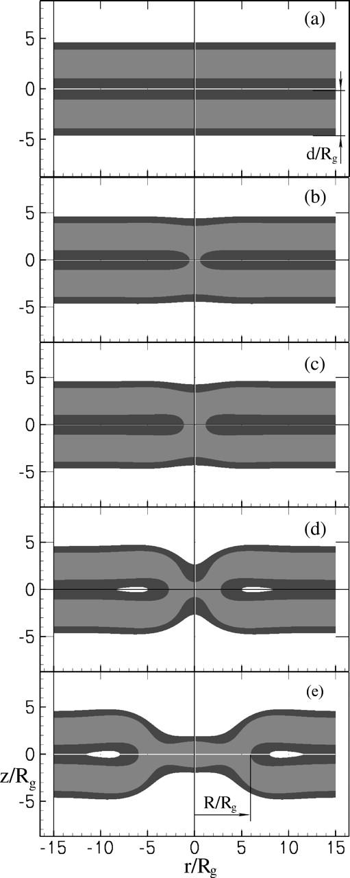
Density profiles of the stalk-like structures shown in the (r, z) plane of cylindrical coordinates. As the structures are axially symmetric, the figure and its reflection about the z axis are shown for the viewer's convenience. The amphiphiles contain a fraction f = 0.35 of the hydrophilic component. The bilayers are under zero tension. Only the majority component is shown at each point: solvent segments are not shown; hydrophilic and hydrophobic segments of the amphiphile are dark and light shaded, correspondingly. Distances are measured in units of the polymer radius of gyration, R_g, which is the same for both the amphiphiles and for the homopolymer solvent. (a) Two bilayers in solvent. There is no stalk between them. Their thickness, d, defined in Eq. 4, is shown. (b) Unstable transition state to the formation of the initial stalk, a state we label S₀. The radius of the stalk is R = 0.6 R_g. In general the stalk radius R is defined by the condition on the local volume fractions φ_A(R, 0) − φ_B(R, 0) = 0. (c) The metastable stalk itself, which we label S₁. Its radius is R = 1.2 R_g. (d) The unstable transition state between the metastable stalk and the hemifusion diaphragm. This transition state is denoted S₂. Its radius is R = 2.8 R_g. (e) A small hemifusion diaphragm of radius R = 3.4 R_g. The radius is shown explicitly.

FIGURE 2.

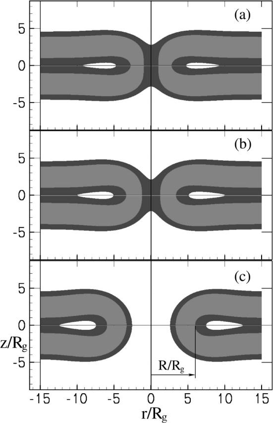
(a) Density profile of a fusion pore of radius R/R_g = 2.4. Were the radius any smaller, the pore would be absolutely unstable to a stalk-like structure. In general the pore radius is the larger value of the radial coordinate that satisfies the condition on the local volume fractions φ_A(R, 0) − φ_B(R, 0) = 0. (b) A pore of radius R/R_g = 3.4 and (c) one of radius R/R_g = 6.0. The radius is shown explicitly. The hydrophilic fraction of the amphiphile, f = 0.35, as in Fig. 1 and the tension is zero, again as in Fig. 1. Distances are measured in units of the radius of gyration R_g.

The most notable results of our calculation are:

1. The free energy barrier to form a stalk, that is, the free energy difference between the initial configuration of Fig. 1 a and that of the transition state Fig. 1 b, is small—on the order of 10 k_BT, much smaller than the estimates of phenomenological theories (Kuzmin et al., 2001).

2. The more important fusion barrier is encountered on the path between the metastable stalk (Fig. 1 c), through another transition state (Fig. 1 d), to a small hemifusion diaphragm (Fig. 1 e). The height of this barrier depends strongly on both the effective spontaneous curvature of the amphiphile and the membrane tension. As expected, the barriers to fusion are reduced as the architecture is changed so as to approach the transition from the lamellar to the inverted-hexagonal phases. The effect of tension on the barriers to fusion is less dramatic, but still very important.

3. We find that the hemifusion diaphragm does not expand appreciably before converting to the fusion pore.

4. The small fusion pore formed by rupturing the hemifusion diaphragm can, at low tension, be trapped in a metastable state and not expand further. This result provides an explanation for the flickering fusion events that are observed experimentally. As the tension is increased, however, this metastable state disappears and the fusion pore, once formed, expands without limit, thus resulting in complete fusion.

5. We observe that the regime of successful fusion is rather severely limited by the architecture of the lipids. If their effective spontaneous curvature is too negative, fusion is pre-empted by the formation of either an inverted-hexagonal phase or a stalk phase. If their curvature is not sufficiently negative, fusion is prevented by the absence of a metastable stalk.

We discuss these results further in Discussion.

THE MODEL

We consider a system consisting of an incompressible mixture of two kinds of polymeric species contained in a volume V. There are n_a amphiphilic diblock copolymers, composed of A (hydrophilic) and B (hydrophobic) monomers, whereas the n_s solvent molecules are represented by hydrophilic homopolymers consisting of A segments only. The fraction of hydrophilic monomers in the diblock is denoted f, and the identical polymerization indices of both the copolymer and the homopolymer are denoted N. The hydrophilic and hydrophobic monomers interact with a local repulsion of strength χ, the Flory-Huggins parameter. Provided that these parameters are chosen appropriately, this model is essentially equivalent to that which we simulated earlier (Müller et al., 2003b). We emphasize that the earlier simulation and the calculation presented here are completely independent. Comparison of results obtained from the two different calculations, therefore, are instructive.

The partition function of the system of flexible chains with Gaussian chain statistics can be formulated easily in either canonical or grand canonical ensembles (Matsen, 1995; Schmid, 1998), but is too difficult to be evaluated analytically. Consequently we employ the well-established SCFT, to obtain a very good approximation to the partition function. This theory has been recently reviewed (Schmid, 1998), so we relegate to the Appendix a brief reminder of the salient features of the approximation. It suffices here to say that the inhomogeneous systems we shall be studying are characterized by a local volume fraction of hydrophilic units, φ_A, and of hydrophobic units, φ_B. Due to the incompressibility constraint, these two volume fractions add to unity locally. It is convenient to control the relative amounts of amphiphile and of solvent, and therefore the relative amounts of A and B monomers, by an excess chemical potential Δμ, the difference of the chemical potentials of amphiphile and of solvent. Within this ensemble, the SCFT produces a free energy, Ω, which is a function of the temperature, T, the excess chemical potential, Δμ, the volume V, and, when bilayers are present, the area A that they span. In addition, the free energy is a function of the local volume fractions φ_A and φ_B, which are obtained as solutions of a set of five nonlinear, coupled equations, given in Eqs. 8–12. Acceptable solutions are defined by various constraints. For example, we require that all solutions be axially symmetric, an assumption embedded in all previous treatments of the stalk/hemifusion process. We take the axis of symmetry to be the z axis of the standard cylindrical coordinate system (r, ϕ, z). Further, we require all solutions to be invariant under reflection in the z = 0 plane. Thus φ_A(r, ϕ, z) → φ_A(r, z) = φ_A(r, −z), and similarly for φ_B. Other constraints are more interesting. For example, to describe a stalk-like structure, as in Fig. 1, we require that the solution display a connection, along a portion of the z axis, between the hydrophobic portions of the two bilayers. Further, we constrain its radius, R, defined by the condition φ_A(R, 0) = φ_B(R, 0), to be a value specified by us. In this way we are able to calculate the free energy of stalk-like structures as a function of their radius. To reiterate, once a solution of the set of nonlinear coupled equations is found which, for given temperature, excess chemical potential and volume satisfies the various constraints imposed, the free energy within the SCFT follows directly. We now turn to a description of the results of this procedure for the systems of interest. We begin with those obtained for isolated bilayers.

PROPERTIES OF ISOLATED BILAYERS

Here we present a range of microscopic and thermodynamic properties of isolated bilayer membranes in excess solvent that follows from our calculation. The most basic structural properties of the bilayer membrane are the distribution of the hydrophilic and hydrophobic segments across it. In Fig. 3 we present the composition profiles obtained within the SCFT approach, shown by solid lines, and compare them to those obtained from our independent simulations (Müller et al., 2003b), which are shown by the symbols. The profiles from simulation are averaged over all configurations. In the Monte Carlo simulation we used amphiphilic polymers consisting of 11 hydrophilic and 21 hydrophobic monomers. This corresponds to a hydrophilic fraction f = 11/32 ≈ 0.34, the value we also used in the SCFT calculations. Fig. 3 corresponds to a system under zero tension. The profiles change quantitatively, but not qualitatively, as the tension is increased.

FIGURE 3.

Results from SCFT (solid lines) for the composition profile across a bilayer membrane that is under zero tension. For comparison, the profile obtained independently from simulation by averaging over configurations is shown in symbols. The hydrophilic fraction of the amphiphiles is f = 0.34.

The overall agreement between the SCFT and averaged Monte Carlo simulation results is very good. The position and the width of the regions enriched in A (head) and B (tail) segments of the amphiphile and solvent segments are reproduced quantitatively in the SCFT model. The small discrepancies in the A/B interfacial width can be attributed to capillary waves and peristaltic fluctuations present in the Monte Carlo simulations, but neglected in the SCFT calculations.

Thermodynamic properties of the bilayer can be calculated from the free energy of the system that contains such a bilayer of area We denote this free energy Ω_m(T, Δμ, V, 𝒜). Similarly, we denote the free energy of the system without the membrane, i.e., a homogeneous amphiphile solution, Ω₀(T, Δμ, V). The difference between these two free energies, in the thermodynamic limit of infinite volume, defines the excess free energy of the membrane,

(1)

The excess free energy per unit area, in the thermodynamic limit of infinite area, defines the lateral membrane tension

(2)

In the grand canonical ensemble this tension γ can be related to the temperature and chemical potential by means of the Gibbs-Duhem equation

(3)

where δs is the excess entropy per unit area, and δσ_a is the excess number of amphiphilic molecules per unit area. This relation is quite useful because it shows that one can set the tension to any given value by adjusting the excess chemical potential of amphiphiles at constant temperature.

Depending on the applied tension, the thermodynamic behavior of the membrane can be classified into three generic types. For values of the tension that are sufficiently small and positive, the membrane is metastable with respect to rupture, and it is this range of tension that we consider below. For larger positive values of γ, the membrane becomes absolutely unstable to rupture, whereas for negative γ, the system is unstable to an unlimited increase in the membrane's area, which simply leads to formation of the bulk lamellar phase. In the following, we shall use the dimensionless tension, γ/γ_int, where γ_int is the interfacial free energy per unit area between coexisting solutions of hydrophobic and hydrophilic homopolymers at the same temperature.

The dependence of the membrane thickness,

(4)

and membrane tension, γ, on the exchange chemical potential is shown in Fig. 4. The agreement is excellent between the SCFT predictions and the independent simulation results averaged over all configurations. From the membrane tension, the area compressibility modulus, κ_A, can be obtained by using any of the equivalent relations,

(5)

Most of the earlier treatments of membranes relied on elasticity theory, in which a membrane is described solely by its elastic properties, such as the bending modulus, κ_M, the saddle-splay modulus, κ_G, and the spontaneous curvature, c₀ (Safran, 1994). These moduli are normally taken either from an experimental measurement or from a microscopic theory. The SCFT approach, being based on a microscopic model, allows one to calculate these moduli in a straightforward manner that can be sketched as follows.

FIGURE 4.

Bilayer thickness, d, measured in units of the radius of gyration R_g with scale to left, versus excess chemical potential as obtained in our SCFT calculation (solid line). This result is compared to that of an independent simulation averaged over all configurations (solid circles). Also shown is the excess free energy per unit area, or tension, of the bilayer, scale to the right, as a function of the exchange chemical potential. Results obtained in our SCFT calculation are shown by the solid line, and those obtained in an independent simulation are shown by the dotted line. The error bar shows the uncertainty in the exchange chemical potential at which the bilayer is without tension as determined in the simulations.

One calculates within the SCFT the excess free energies due to small spherical and cylindrical deformations of an interface containing an amphiphilic monolayer. These excess free energies depend upon microscopic parameters, such as the amphiphile hydrophilic fraction f, as well as the curvatures of the deformations. They are then fit to the standard Helfrich-Hamiltonian of an infinitely thin elastic sheet, which depends upon phenomenological parameters, and the curvatures of the deformations. This Hamiltonian for a saturated, tensionless monolayer is (Safran, 1994)

(6)

where M and G are the local mean and Gaussian curvatures of the deformed monolayer. From the fit, one obtains the phenomenological parameters in terms of the microscopic quantities. Details of this procedure can be found in Matsen (1999) and Müller and Gompper (2002). Because SCFT ignores fluctuations, the moduli obtained are the bare, un-renormalized values. The effect of renormalization is usually small (Peliti and Leibler, 1985) and depends on the lateral length scale of the measurement. Fusion proceeds on a lateral length scale that does not exceed the membrane thickness by a great deal and, on this length scale, we expect the renormalization of the elastic constants to be small.

In Fig. 5 a we show the calculated spontaneous curvature of an amphiphilic monolayer as a function of the hydrophilic fraction f of the amphiphile. The former is a monotonic function of the latter. This is to be expected, as the phenomenological spontaneous curvature attempts to capture some of the effects of the differing hydrophilic and hydrophobic volumes in the amphiphile, which are specified by f, on the membrane configurations. The above result provides a direct mapping between the phenomenological property c₀, which can be measured experimentally (Rand et al., 1990; Leikin et al., 1996) and the microscopic variable f used in our calculations. Our results for the area compressibility, κ_A, and elastic moduli κ_M and κ_G are shown in Fig. 5 b. In agreement with experiments on model lipid systems, they are not very sensitive to changes in amphiphile architecture parameter f or, equivalently, to the spontaneous curvature c₀. For comparison with our model system, we present in Table 1 the properties of lipid and amphiphilic diblock membranes determined experimentally.

FIGURE 5.

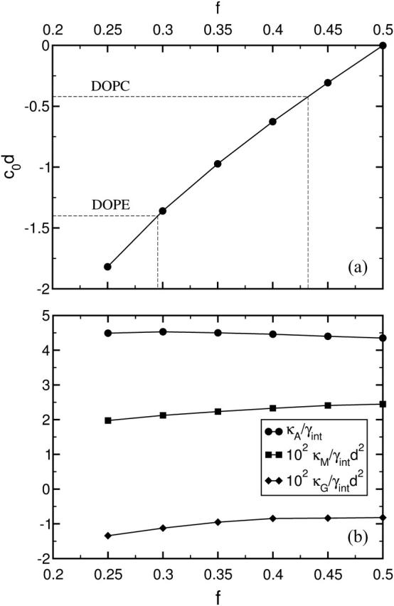
(a) Dependence of the product of spontaneous curvature and bilayer thickness, c₀d, on hydrophilic fraction f of the amphiphile. Experimental values of c₀d for DOPE and DOPC from Table 1 and the corresponding values of f are shown. (b) Plot of the dependence of dimensionless values of the area compressibility, κ_A, bending modulus, κ_M, and saddle-splay modulus, κ_G, moduli on the hydrophilic fraction f of the amphiphile.

TABLE 1.

Structural and elastic properties of bilayer membranes

	Polymersomes	Liposomes
	EO7	DOPE	DOPC
d	130 Å	38.3 Å*	35.9 ņ
c0d	no data	−1.4§	−0.42‡
κA/γint	2.4	4.4†	2.9†
κM/γintd2 × 102	1.67	6.0‡	6.0§

Key: d, bilayer membrane thickness; c₀, monolayer spontaneous curvature; κ_A, bilayer area compressibility modulus; κ_M, monolayer bending modulus; γ_int = 50 pN/nm, oil/water interfacial tension. Data on EO7 polymersomes is taken from Discher et al. (1999). Values of d, c₀, and κ_a for DOPE were obtained by linear extrapolation from the results on DOPE/DOPC(3:1) mixtures and pure DOPC.

^*From Rand and Parsegian (1989).

^†From Rand et al. (1990).

^‡From Chen and Rand (1997).

^§From Leikin et al. (1996); see also http://aqueous.labs.brocku.ca/lipid//.

Lipid membranes are known to exhibit strong mutual repulsion at small separations, usually attributed to so-called hydration forces (Parsegian and Rand, 1994). We calculated the free energy of a system containing two planar bilayers in excess solvent under the condition that the distance between the cis interfaces be constrained to a given value. This technique has been used before to study monolayer interactions in a similar system (Thompson and Matsen, 2000), and we refer the reader to this article for details.

One finds that there are two generic features of the free energy of the two bilayers as a function of their separation. First at sufficiently small separation, when heads of the amphiphiles come in contact, the membranes experience strong repulsion due to this contact, a repulsion that rises steeply as the separation is further reduced. Second at a somewhat larger separation, there is a very weak attraction between the two membranes. These two features have been exhaustively analyzed (Thompson and Matsen, 2000). It has been determined that the repulsion arises mostly from the direct steric interaction between the head segments of the amphiphiles in the contacting cis monolayers. The weak attraction occurs because the solvent molecules prefer to leave the confining intermembrane gap to increase their conformational entropy. This is simply the well-known depletion effect, about which there is a very large literature (Götzelmann et al., 1998). The combination of the short-range repulsion and the depletion effect attraction produces a minimum in the free energy at some separation. The distance at which this minimum occurs, typically on the order of one R_g between opposing cis leaves, is the equilibrium separation.

The reasonable description of the properties of self-assembled monolayers and bilayers presented above provides confidence that our model can be used to describe the structural changes that occur in membranes during the fusion process.

ENERGETICS OF THE STALK AND OF ITS RADIAL EXPANSION

The formation and stability of the initial interconnection between the membranes, the stalk itself, has not received much theoretical attention. Creating the stalk requires the membranes to undergo drastic topological changes, which cannot be easily described by continuum elastic models. The common approach has been to assume that two small hydrophobic patches (one in each membrane) are produced by thermal fluctuations in the region of contact. Hydrophobic interactions then drive the connection of these energetically costly regions, and result in the formation of a metastable structure, the stalk (Markin and Kozlov, 1983). The size of the hydrophobic patches and the distance between them can be optimized to minimize the free energy of the unstable transition state. With the use of this strategy, continuum elastic models have estimated the free energy barrier to create a stalk to be ∼37 k_BT (Kuzmin et al., 2001). The SCFT method allows us to obtain solutions for both the unstable transition state to stalk creation and for the stalk itself, if it is indeed metastable.

The dependence of the free energy of stalk-like structures on their radius, R, when the bilayers in which they form are under zero tension, is shown in Fig. 6 a. It is plotted for various values of the architectural parameter, from f = 0.45, which corresponds to an amphiphile with a very small negative spontaneous curvature, to f = 0.25, an amphiphile with a large negative spontaneous curvature. From Fig. 5 a it is seen that this f-range includes DOPC and DOPE lipids, which are frequently utilized as components of model lipid membranes in fusion experiments. At f = 0.45 we could not find a stalk-like solution for 2.2 < R/R_g < 4. The system would spontaneously rupture in the vicinity of the symmetry axis r = 0, resulting in a fusion pore-like structure.

FIGURE 6.

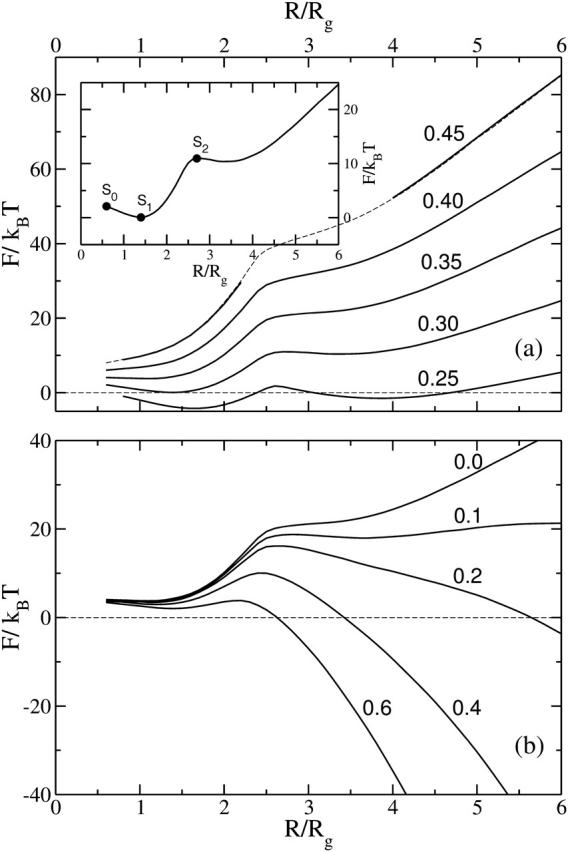
(a) The free energy, F, of the stalk-like structure connecting bilayers of fixed tension, zero, is shown for several different values of the amphiphile's hydrophilic fraction f. In the inset we identify the metastable stalk, S₁, the transition state, S₀, between the system with no stalk at all and with this metastable stalk, and the transition state, S₂, between the metastable stalk and a hemifusion diaphragm. The architectural parameter is f = 0.30 for this inset. No stable stalk solutions were found for f = 0.45 in the region shown with dashed lines. They were unstable to pore formation. (b) The free energy of the expanding stalk-like structure connecting bilayers of amphiphiles with fixed architectural parameter f = 0.35 is shown for several different bilayer tensions. These tensions, γ/γ_int, are shown next to each curve.

The extremal points of the free energy of the system with a stalk-like structure with respect to its radius correspond to intermediate structures and transition states. The free energy extrema of the intermediates are saddle points with respect to deformations, and are therefore unstable, whereas those of the intermediates are local minima, and are therefore metastable. In the inset to Fig. 6 a we identify three states with extremal free energies. Depending on the values of the architecture parameter f and the membrane tension γ, we find the following solutions playing central roles in the description of the membrane fusion process:

• The transition state between the unperturbed bilayers and the metastable stalk, S₀.

• The metastable stalk itself, S₁.

• The transition state that occurs as the initial small stalk is radially expanded into the hemifusion diaphragm, denoted S₂.

It is clear from Fig. 6 a that the metastable stalk solution S₁ (and therefore the transition state S₀) exists only for sufficiently small values of the hydrophilic fraction f. At zero membrane tension this minimal f is ∼0.36, which corresponds to the spontaneous curvature c₀d = −0.9, approximately that of a 1:1 mixture of DOPE and DOPC lipids. To our knowledge, this is the first theoretical prediction of the metastability of the stalk itself. Existence of the stalk intermediate is crucial for the fusion dynamics, since it separates the fusion process into two activated stages: creation of the stalk and its further expansion. We argue, therefore, that for those conditions, specified by f and γ, under which there is no S₁ solution, fusion will be considerably slower or, perhaps, impossible. Fig. 6 a also shows that, at small stalk radius, R, the free energy barrier to create the stalk, which corresponds to the state S₀, does not exceed 5 k_BT. This value is much smaller than the 37 k_BT predicted by the phenomenological calculation (Kuzmin et al., 2001). Of course, one can ask how applicable our results for block copolymer membranes are to biological ones. If we take as a natural measure of energy the dimensionless quantity γ_intd²/k_BT, where d is the membrane thickness, we obtain a value of ∼60 in our system, a factor of 2.5 less than that (≈150) for a typical biological bilayer. This suggests that our energies should be scaled up by a factor of ∼2.5 to compare them with those occurring in biological membranes. Even after doing so, however, they are still much smaller than the estimates of the phenomenological theories. We infer from this result that the phenomenological approaches, based on the continuum elastic description, are not accurate in describing the drastic changes in membrane conformations on the length scales comparable to the membrane thickness.

In Fig. 1 b, we show the calculated density profiles of the different segments in the unstable transition state structure S₀ at f = 0.35 and γ/γ_int = 0. As can be seen, the interface between A and B segments is extremely curved, and the stalk radius R = 0.6 R_g is much smaller than the membrane hydrophobic core thickness. For clarity, we show only the majority component at each point. The interfaces between the different components appear to be sharp in such a graphical representation, but actually they are relatively diffuse, as can be seen in Fig. 3.

The behavior of the free energy of the stalk-like structure as it expands into a hemifusion diaphragm under non-zero tension is shown in Fig. 6 b, and one clearly sees a second local maximum at R/R_g ≈ 3 that corresponds to the second unstable transition state, S₂. The maximum results from the competition between the elimination of the energetically costly bilayer area, which reduces the free energy as −γπR², and the creation of diaphragm circumference, which increases it as 2πλ_triR. Here λ_tri is a line tension. Fig. 6 b shows that this second maximum is, in general, much greater than that encountered in creating the stalk itself. Therefore we infer that crossing this barrier is the rate-limiting step of the hemifusion mechanism. As the tension increases, the height of this barrier decreases. Thus at very high tension, on the order of 0.5γ_int for f = 0.3, this local maximum disappears entirely, leading to stalk expansion without any barrier at all. The rather strong dependence of this barrier height on tension contrasts with the behavior of the free energy of the metastable stalk itself, which, from Fig. 6, is seen to depend only weakly on the tension. We also note that the minimum in the free energy corresponding to the metastable stalk is exceedingly shallow. This means that these interconnections are easily reversible, and would constantly fluctuate in size.

We recapitulate, in Fig. 7, the dependence of the free energy of the metastable stalk S₁, and of the unstable transition state S₂ on the tension, γ, and on the architectural parameter f. The free energy of the metastable stalk, S₁, varies greatly with f, and decreases substantially for smaller f, i.e., as the spontaneous curvature of the amphiphile becomes more negative. Although our calculation applies to membranes composed of a single amphiphile, and not a mixture, it clearly strengthens the argument that one role of such negative curvature lipids as phosphatidylethanolamine, present in the plasma membrane, is to make metastable and thermally accessible the formation of stalks, which are necessary to begin the fusion process (de Kruijff, 1997). For sufficiently small values of the architectural parameter f, the free energy of the metastable stalk actually becomes lower than that of the unperturbed bilayers. Presumably this leads to the formation of the thermodynamically stable “stalk phase” recently realized experimentally in a lipid system (Yang and Huang, 2002).

FIGURE 7.

The free energy, F, of the metastable stalks S₁ (dashed lines) and the transition states S₂ (solid lines) as a function of the tension for different architectures f = 0.25, 0.30, 0.35, and 0.40. Note that there is no S₁ solution for f = 0.4 at the values of tension we studied.

In summary, both an increase in the membrane tension γ and a decrease in the hydrophilic fraction f favor stalk expansion into the hemifusion diaphragm. The density profiles in the transition state between the metastable stalk and the hemifusion diaphragm are shown in Fig. 1 d, and that of the unstable, expanding, hemifusion diaphragm in Fig. 1 e. Note how thin is the hydrophobic region on the axis of symmetry in Fig. 1 d and next to the triple junction in Fig. 1 e, compared to the thickness of the bilayers away from the diaphragm.

FORMATION AND EXPANSION OF FUSION PORE

The hemifusion diaphragm is a possible intermediate along the path to fusion, but for complete fusion to occur, a hole must nucleate in the diaphragm leading to the formation of the final fusion pore. Here we consider the energetics of the fusion pore. The manner in which we obtain solutions corresponding to the pore and determine its free energy are similar to those for the stalk described above. A density profile of a fusion pore is shown in Fig. 2 a. In the plane of mirror symmetry between the two bilayers, there are two radii at which the volume fraction of hydrophobic and hydrophilic elements are equal, i.e., for which φ_A(r, 0) − φ_B(r, 0) = 0. We define the radius, R, of the fusion pore as the greater of these two distances. This choice is consistent with the definition of the radius of a stalk-like structure, the only radius at which φ_A(r, 0) − φ_B(r, 0) = 0, as can be seen from the following: if one begins with a stalk-like structure of radius R and introduces a hole into it to create a pore, then the radius of the pore, according to the above definition, is also R, as it should be. We are able, therefore, to directly compare the free energies of the pore and stalk-like structures with the same radius.

The free energy of the fusion pore in a system with fixed architecture, f = 0.35, but under various tensions is shown in Fig. 8. As the tension on the membrane is increased from zero, the free energy of the pore decreases as −2γπR² for large radius R, similar to the free energy decrease of the hemifusion diaphragm. The factor of 2 arises because pore expansion eliminates both membranes, whereas hemifusion expansion removes only one.

FIGURE 8.

The free energies, F, of a fusion pore (solid lines) and of a stalk (dashed lines, compare to Fig. 6 b) of radius R are shown. Under the assumption that the stalk-like structure converts to a fusion pore when their free energies cross, one can read off the barrier between metastable stalk and formation of the fusion pore. The membranes are comprised of amphiphiles with fixed architecture, f = 0.35, and are under various tensions γ/γ₀ as indicated in the key. Note that the fusion barrier decreases with increasing tension.

The free energies of the fusion pores, shown in solid lines in Fig. 8, are compared with those of the stalk-like structures under the same conditions, which were shown previously in Fig. 6 b. We assume that a hole forms in the hemifusion diaphragm converting the diaphragm into a fusion pore when the free energy of the pore becomes lower than that of the stalk-like structure. The radius at which the free energies of the expanding stalk and of the fusion pore become equal is R ≈ 2.5–3.5 R_g. Of course, there is not a sharp transition from the stalk to the pore, because the free energies are finite. There is instead a region of radii where the transition from the stalk to the fusion pore occurs, and which is characterized by a free energy difference of the order of thermal fluctuations k_BT. Because the stalk and pore structures are so similar at such small values of radius, it is likely that there is only a very small free energy barrier associated with rupture of the hemifusion diaphragm, which converts it to the fusion pore. Therefore, our calculations indicate that the hemifusion diaphragm would hardly expand before the fusion pore would form. This agrees with the conclusion of a recent phenomenological calculation (Kuzmin et al., 2001).

Fig. 8 shows that, except at low tension, the hole forms in the diaphragm after the barrier to diaphragm expansion has been crossed. Therefore within the standard hemifusion mechanism, the barrier to hemifusion expansion is, in fact, the major barrier to fusion.

At very low tensions, our results show that the most important barrier to fusion is no longer that governing the expansion of the hemifusion diaphragm, but becomes that associated with the expansion of the fusion pore itself. As a consequence of the large barrier to expansion of the fusion pore, pores of small radius, R ≈ 3.4 R_g, become metastable for most architectures for tensions γ/γ₀ <∼0.1. This metastability persists to zero tensions, as seen from Fig. 9. Note that the potential minimum of the metastable pore is quite shallow, therefore one would expect that thermal fluctuations will easily cause it to expand and contract, or flicker, at the minimum free energy configuration with an amplitude of the order of 1 R_g. Note also that the activation barrier to reseal the fusion pore is quite substantial, on the order of 5 k_BT, which would translate to ∼13 k_BT in lipid systems. This means that flickering pores can be long-lived metastable states and, depending on the tension, might either reseal or expand. In retrospect, it should not be surprising that a small fusion pore is metastable in a tensionless membrane. Its free energy must increase linearly with its radius due to the line tension cost of its circumference. On the other hand as its radius decreases, the pore eventually becomes sufficiently small so that the inner sides of the pore come into contact, repelling each other and causing the free energy to again increase. Thus there must be a minimum at some intermediate distance. If the radius is decreased below some critical value, the compressed pore structure becomes unstable to the stalk-like structure. This instability is shown with arrows in Fig. 9. The density profile of such a marginally stable pore occurring in a membrane with f = 0.35 and R = 2.4 R_g is shown in Fig. 2 a.

FIGURE 9.

The free energies, F, of a fusion pore (solid lines) and of a stalk (dashed lines) of radius R are shown. In contrast to Fig. 8, the membranes here are under zero tension, and are comprised of amphiphiles with various values of f. The instability of the fusion pores at small radius is indicated by arrows. For f = 0.3, 0.35, and 0.4, the stalk-like structure converts into a pore when it expands to a radius R ≈ 2.4 R_g at which the free energies of stalk-like structure and pore are equal. For the system composed of amphiphiles of f = 0.25, however, the stalk-like structure converts at R ≈ 2 R_g into an inverted micellar intermediate (IMI), whose free energy is shown by the dotted line. The fusion pore is unstable to this IMI intermediate when its radius decreases to R ≈ 3.4 R_g. Thus the IMI is the most stable structure under these conditions.

Fig. 9 shows that the small flickering pore would be thermally excited from a metastable stalk for most of the architectures shown, f = 0.40, 0.35, and 0.30. As the architecture changes such that f decreases still further, the stalk free energy becomes negative—meaning that it is favorable to create many of them, which leads to the formation of a stalk phase. This occurs for non-zero tension as well.

Lastly, we note from Fig. 9 that at very low tension and very small values of the architectural parameter (f = 0.25, corresponding to a large and negative spontaneous curvature), both the fusion pore and the stalk-like structure are unstable to another structure, the inverted micellar intermediate (IMI), introduced by Siegel (1986). Interestingly, this configuration was suggested previously as a possible player in the fusion process, but has been largely neglected because free energy estimates obtained from elastic approaches were prohibitively high. As will be shown in our second article, the IMI and related linear stalk intermediates are very important in describing fusion.

DISCUSSION

We have carried out a self-consistent field study of the fusion of membranes consisting of flexible block copolymers in a solvent of homopolymer. The main purpose of this article was to evaluate the free energy barriers encountered within the standard hemifusion, or stalk, mechanism. We summarize our major findings in Fig. 10 in a phase diagram depicting the parameter space of amphiphile architecture and tension.

FIGURE 10.

A phase diagram of the hemifusion process in the hydrophilic fraction-tension, (f, γ), plane. Circles show points at which previous independent simulations were performed by us. Successful fusion can occur within the unshaded region. As the tension, γ, decreases to zero, the barrier to expansion of the pore increases without limit as does the time for fusion. As the right-hand boundary is approached, the stalk loses its metastability, causing fusion to be extremely slow. As the left-hand boundary is approached, the boundaries to fusion are reduced, as is the time for fusion, but the process is eventually pre-empted due to the stability either of radial stalks (forming the stalk phase), or linear stalks (forming the inverted hexagonal phase).

We find that as the architecture of the amphiphile f is changed so that its spontaneous curvature decreases from zero and becomes more negative, fusion is enhanced. There are at least two reasons for this. First, the initial stalk becomes metastable only if f is sufficiently small (i.e., the spontaneous curvature is sufficiently negative). This is the case in the region to the left of the nearly vertical black dashed line in Fig. 10. Presence of the metastable stalk intermediate is crucial for fast fusion, because its formation represents the first of at least two activated steps in the fusion process. Within the hemifusion mechanism, the second activated step is the radial expansion of the stalk into a hemifusion diaphragm. We expect that in the region in which the stalk is not metastable, fusion would be extremely slow, if not impossible.

We also find that for a sufficiently small f the stalk intermediate becomes absolutely stable with respect to the system with unperturbed membranes. There is a small region (shown in the figure between the dotted and solid lines) in which the stalk is not only stable with respect to the unperturbed system, but is more stable than any other intermediate we have considered. Consequently we predict formation of a “stalk phase” in this region. This result is in accord with recent experiments on model lipid systems (Yang and Huang, 2002). As the spontaneous curvature is made even more negative, linear stalks, which are precursors to the formation of an inverted-hexagonal phase, become even more stable than radial stalks. Hence the stalk phase becomes unstable with respect to the inverted hexagonal phase.

We remark that, according to our calculations on bilayers comprised of a single amphiphile, the variation of architectures within which successful fusion can occur is quite small. One way that a system composed of many different amphiphiles can ensure the appropriate effective architecture is to employ a mixture of lipids comprised of those with small spontaneous curvatures, or lamellar formers, and those with larger negative spontaneous curvatures, or nonlamellar formers. Further, to remain within the small region of successful fusion, the ratio of these different kinds of lipids must be regulated, as indeed it is (Morein et al., 1996; Wieslander and Karlsson, 1997).

We also note that the restrictions we have found on the possible variation of curvature, if fusion is to be successful, arise from stability arguments involving the stalk itself. Therefore any fusion mechanism that begins with the formation of a stalk will have this same phase diagram even though the subsequent path to fusion may differ radically from the standard hemifusion mechanism.

Within the range of the parameters where fusion can occur, we find that the activation barriers of the three major stages of the standard hemifusion process, which are stalk formation, stalk expansion, and pore formation, are affected differently by changes in architecture and in tension. The first activation barrier is associated with creation of the initial metastable stalk. Its height is essentially independent of the membrane tension and increases only very weakly as f is increased. Stalk creation is apparently not a rate limiting step, because the corresponding barrier does not exceed 5 k_BT in our model, or 13 k_BT if we extrapolate our results to lipid systems. This value is much lower than previous estimates of phenomenological theories (Kuzmin et al., 2001).

In the second stage, during radial stalk expansion, the corresponding barrier is a very sensitive function of the amphiphile architecture, as can be seen in Fig. 7. At small tension it ranges from ≈10 k_BT for amphiphiles with small f up to ≈25 k_BT for more symmetric amphiphiles. Again, this range translates into 25–63 k_BT for biological bilayers. These observations are consistent with well-known fusion enhancement effects of lipids with large and negative spontaneous curvature, such as DOPE, when they are added to fusing membranes (Chernomordik et al., 1995; Chernomordik, 1996). The effect of membrane tension on the stalk expansion barrier has also been determined. We find that increased tension lowers the activation barrier to radial stalk expansion and pore formation. This is in accord with experiment (Monck et al., 1990). We predict that this barrier to fusion can, in principle, always be reduced and eliminated by sufficient tension. However, if the architecture of the amphiphiles is unfavorable, resulting in a very high barrier at zero tension, the tension needed to eliminate this barrier can be prohibitively high, and fusion will be pre-empted by membrane rupture. Results on the thermodynamics of membrane rupture will be presented in the second article of this series.

The third stage of the process, nucleation of a hole in the diaphragm to convert the hemifusion diaphragm into a fusion pore and the pore's expansion, appears to present no additional barrier to fusion at most non-zero tensions. Thus we find that the largest barrier encountered in this standard hemifusion mechanism is that associated with the expansion of the stalk into a hemifusion diaphragm. The diaphragm does not expand very much, however, before this maximum barrier is reached.

At very low tensions, the controlling barrier is that associated with the expansion of the fusion pore. This leads to the prediction of the transient stability of small fusion pores. We believe that these structures correspond to “flickering pores” observed experimentally in lipid bilayer fusion (Fernandez et al., 1984; Spruce et al., 1990; Chanturiya et al., 1997).

Despite the agreement between our results on the hemifusion mechanism and the experimental observations mentioned above, there remain experimental observations that this hypothesis does not explain. First, lipid mixing is observed to occur not only between the cis monolayers, but also between cis and trans layers (Lentz et al., 1997). Second, transient leakage is observed, and it is correlated spatially and temporally with fusion (Frolov et al., 2003). In addition to these experimental observations, simulation studies have revealed, both in planar bilayer fusion and in vesicular fusion, a very different pathway subsequent to the formation of the initial metastable stalk. To understand these discrepancies, we have performed calculations similar to those presented here for the alternative mechanism recently proposed by Noguchi and Takasu (2001) and Müller et al. (2002b, 2003b). These results will be presented in the second article of this series.

APPENDIX A: SELF-CONSISTENT FIELD THEORY FOR POLYMER SYSTEMS

The first step in any field-theoretic approach to such systems is to convert the partition sum over all possible molecular configurations into an integration over configurations of corresponding, smooth, collective variables, the density and chemical potential fields. The derivation of the effective field-theoretic Hamiltonian of our polymer model follows a standard prescription, so we give only the final expression here:

(7)

Here z ≡ exp(Δμ/k_BT) is the relative activity of the amphiphiles, where Δμ = μ_a − μ_s, the difference in bulk chemical potentials of the amphiphile and the solvent. There is only one independent chemical potential because the liquid is assumed to be incompressible. The fixed number density of polymer chains, (n_a + n_s)/V, is denoted Φ. Thus the total number density of chains is fixed, but the relative amounts of amphiphile and solvent chains is controlled by the chemical potential difference, Δμ. The Flory interaction parameter, χ, is inversely proportional to the temperature. The Q_s[w_A] and Q_a[w_A, w_B] are the single chain partition functions of the solvent and amphiphile molecules subjected to the local chemical potential fields, w_A(r) and w_B(r), which act on the A and B segments, respectively. The local volume fractions of A and B monomers are given by φ_A(r) and φ_B(r). The “local pressure” ξ(r) is the Lagrange multiplier field introduced to enforce the incompressibility condition.

The mean field approximation, which is at the heart of the SCFT approach, amounts to extremizing the field-theoretic Hamiltonian with respect to all the fields upon which it depends. Fluctuations at this extremum are ignored. In systems of relatively long chains, in which composition fluctuations are small, the results of this approximation are very good indeed (Bates and Fredrickson, 1999).

It can be shown that the field configurations that correspond to stationary points of denoted in the following by an over-bar, satisfy the following set of coupled nonlinear equations:

(8)

(9)

(10)

(11)

(12)

where the single chain propagators q_c(r, s), and q_s(r, s) satisfy the usual modified diffusion equations for the flexible polymer chains with the Gaussian statistics; e.g., for the homopolymer solvent it is

(13)

Here R_g is the radius of gyration of the unperturbed Gaussian polymer. The value of the free energy of the stationary configuration is given simply by

(14)

The system of nonlinear equations (Eqs. 8–12) together with the equations for the propagators (Eq. 13) can be solved numerically in real space by a straightforward relaxational iterative algorithm (Drolet and Fredrickson, 1999). The real-space approach has far more flexibility in studying localized structures, such as the fusion intermediates, than does the more numerically optimized spectral approach (Matsen and Schick, 1994). The recently proposed pseudo-spectral techniques (Rasmussen and Kalosakas, 2002) appear to be very efficient, but they rely heavily on the numerical fast Fourier transforms, which are not available for the cylindrical coordinates, r = (r, ϕ, z), that we use in our calculations. Because the local volume fractions are required to be axially symmetric, φ_A(r, z), φ_B(r, z), and to be symmetric under reflection in the z = 0 plane, the problem is two-dimensional and need only be solved in one quadrant. We impose reflecting boundary conditions at z = 0, z = z_max, r = 0, and r = r_max, where z_max and r_max determine the size of the computational cell. They were set to 8 R_g and 15 R_g, respectively. We discretized all the fields on a uniform lattice with resolution Δr = Δz = 0.1 − 0.05 R_g. In solving the diffusion Eq. 13 we used contour length discretization of Δs = 0.01 − 0.001. This gave us an accuracy of no less than 0.1 k_BT in the free energy. On a 1-GHz, Pentium III workstation, ∼5 min were required to obtain convergence for a configuration, φ_A(r, z) and φ_B(r, z), at a given value of f and γ.

To describe a stalk-like structure, the solutions must smoothly connect the hydrophobic regions of the two bilayers. The radius, R, of the stalk, again defined by φ_A(R, 0) − φ_B(R, 0) = 0, must take a value that we specify. To facilitate finding such a solution we apply, at the beginning of our calculations, auxiliary external fields that favor hydrophobic segments along the axis of symmetry between the two trans leaves. After the system assembles into the desired structure, these auxiliary external fields are switched off, and the solution is allowed to relax. Far from the axis of symmetry, the membranes reach their equilibrium separation. Again this minimum is due to the short-range repulsion and the attractive depletion interaction between the bilayers. Once a solution satisfying these constraints is obtained, the free energy of the stalk-like structure is then calculated. It is the difference, at constant chemical potential (or, equivalently, constant tension), between the free energy of the system with two bilayers connected by the stalk-like structure, and that of the two unperturbed bilayers without the interconnection.

APPENDIX B: REACTION COORDINATE CONSTRAINT

The SCFT strategy and its numerical implementation along the lines presented above are capable, in practice, only of identifying thermodynamic, locally stable configurations of the system. To clarify this point, consider the following construction. Suppose we first extremize ℋ with respect to the chemical potential fields w_A(r) and w_B(r), and the incompressibility field ξ(r). Then, at least in principle, we obtain a free energy functional that depends only on the physical density fields φ_A(r) and φ_B(r):

(15)

where we have suppressed the dependence on the thermodynamic variables, T, Δμ, V, and An extremum of is the system's free energy Ω_m. This extremum corresponds to a thermodynamic, locally stable state if, and only if, the matrix of the second derivatives is positive definite in that configuration, i.e., the locally stable configurations correspond to the minima of the free energy density functional To distinguish them from other kinds of solutions, we will refer to these locally stable structures as intermediates.

In studying an activated process, such as membrane fusion, we need to know not only the free energy of the intermediates along some reaction path, but also the properties of the transition states, which correspond to saddle points of the free energy functional Unfortunately, finding a saddle point of a functional poses a serious numerical problem. In particular, commonly used relaxational algorithms prove to be inadequate for this task, because they rely on local stability around a solution, which is obviously lacking at the saddle point. Newton-Raphson type algorithms are capable of finding any extremal points as long as the initial configuration is within the basin of attraction of that point. Unfortunately, we do not know the location of a saddle point in advance, so these methods are also not very practical.

In some cases one can identify the unstable directions of the functional and stabilize it by applying a suitable constraint. As an example, consider a transition state between the stalk and the hemifusion diaphragm. We treat this situation in detail in the main text and use it here simply for illustration. We confine the possible solutions to be axially symmetric and to have a mirror symmetry with respect to z = 0 plane because the unstable mode of either the stalk or diaphragm can be associated with an overall radial contraction or expansion of the structure. We further constrain the solution by requiring that, in the z = 0 plane, the A/B interface (i.e., the locus of points at which φ_A(r) − φ_B(r) = 0) be located on a circle of some specified radius R. This radius plays the role of a reaction coordinate. To impose the constraint, we employ a Lagrange multiplier, ψ_R (Matsen, 1999). The corresponding constrained field-theoretic Hamiltonian is then given by

(16)

The first two SCFT Eqs. 8 and 9 should be modified accordingly to

(17)

and the third equation expressing the local density constraint is supplemented by the additional local constraint of

(18)

where, again, (r, z) are cylindrical coordinates. The Lagrange multiplier ψ_R plays the role of the local chemical potential that couples to the density fields. The solution of the SCFT equations optimizes the free energy with respect to ψ_R as well as the other fields. The same relaxational iterative approach as that used for the nonconstrained case proved to be efficient for solving this modified problem.

In general, for an arbitrary position of the constraint R, the value of the Lagrange multiplier ψ_R is non-zero, which means that the corresponding field configuration is not a solution of the original nonconstrained system. Nevertheless, at the points where ψ_R is zero, the constrained and nonconstrained sets of equations become identical, i.e., an extremum of the constrained free energy functional is also an extremum of the nonconstrained functional.

The free energy of the constrained system, F_R, quite generally, satisfies the following “force balance” equation:

(19)

The condition ψ_R = 0 is equivalent to dF_R/dR = 0, so that the extremal points of F_R as a function of R are also the extremal points of as a function of R. Clearly, a minimum of free energy F_R of the restricted system corresponds to a minimum of whereas a maximum of F_R corresponds to a saddle-point configuration of By scanning a range of R-values, we can identify all the metastable intermediates and unstable transition states along a particular path. Moreover, even those constrained configurations for which ψ_R ≠ 0 have a transparent physical interpretation, and provide a wealth of additional information, are inaccessible by the nonconstrained calculations. For other applications of similar constraints we refer the reader to the literature (Matsen, 1999; Müller et al., 2002a; Duque, 2003).

APPENDIX C: MODEL PARAMETERS

To make a direct comparison with our previous independent Monte Carlo simulations (Müller et al., 2003b), we match corresponding model parameters. The length scale in SCFT calculations is usually set by the polymer radius of gyration R_g. For the polymers in the simulations, the radius of gyration was found to be R_g = 6.93u, where u is the spacing of the cubic lattice into which the simulation volume is divided. Because of the incompressibility constraint, the volume per polymer, V/(n_a + n_s), with n_a and n_s the number of amphiphilic and solvent polymers respectively, enters the SCFT free energy only as a multiplicative factor and in a dimensionless ratio As this ratio was taken to be 1.54 in the simulations, we take the same value in evaluating the SCFT free energy. The energy scale in SCFT is set by the product of the Flory interaction parameter χ and the polymerization index N. It has been shown previously that the choice χN = 30 corresponds to the simulated system (Müller et al., 2003b).

References

- Bates, F., and G. Fredrickson. 1999. Block copolymers—designer soft materials. Phys. Today. 52:32–38. [Google Scholar]
- Chanturiya, A., L. Chernomordik, and J. Zimmerberg. 1997. Flickering fusion pores comparable with initial exocytotic pores occur in protein-free phospholipid bilayers. Proc. Natl. Acad. Sci. USA. 94:14423–14428. [DOI] [PMC free article] [PubMed] [Google Scholar]
- Chen, Z., and R. P. Rand. 1997. The influence of cholesterol on phospholipid membrane curvature and bending elasticity. Biophys. J. 73:267–276. [DOI] [PMC free article] [PubMed] [Google Scholar]
- Chernomordik, L. 1996. Non-bilayer lipids and biological fusion intermediates. Chem. and Phys. Lipids. 81:203–213. [DOI] [PubMed] [Google Scholar]
- Chernomordik, L., M. Kozlov, and J. Zimmerberg. 1995. Lipids in biological membrane fusion. J. Membr. Biol. 146:1–14. [DOI] [PubMed] [Google Scholar]
- de Kruijff, B. 1997. Lipid polymorphism and biomembrane function. Curr. Opin. Chem. Biol. 1:564–569. [DOI] [PubMed] [Google Scholar]
- Discher, B. D., Y.-Y. Won, D. S. Ege, J. C.-M. Lee, F. S. Bates, D. E. Discher, and D. A. Hammer. 1999. Polymersomes: tough vesicles made from diblock copolymers. Science. 284:1143–1146. [DOI] [PubMed] [Google Scholar]
- Drolet, F., and G. Fredrickson. 1999. Combinatorial screening of complex block copolymer assembly with self-consistent field theory. Phys. Rev. Lett. 83:4317–4320. [Google Scholar]
- Duque, D. 2003. Theory of copolymer micellization. J. Chem. Phys. 119:5701–5704. [Google Scholar]
- Evans, K. O., and B. R. Lentz. 2002. Kinetics of lipid rearrangements during poly(ethylene glycol)-mediated fusion of highly curved unilamellar vesicles. Biochemistry. 41:1241–1249. [DOI] [PubMed] [Google Scholar]
- Fernandez, J., E. Neher, and B. Gomperts. 1984. Capacitance measurements reveal stepwise fusion events in degranulating mast cells. Nature. 312:453–455. [DOI] [PubMed] [Google Scholar]
- Frolov, V. A., A. Y. Dunina-Barkovskaya, A. V. Samsonov, and J. Zimmerberg. 2003. Membrane permeability changes at early stages of Influenza hemaglutinin-mediated fusion. Biophys. J. 85:1725–1733. [DOI] [PMC free article] [PubMed] [Google Scholar]
- Götzelmann, B., R. Evans, and S. Dietrich. 1998. Depletion forces in fluids. Phys. Rev. E. 57:6785–6800. [Google Scholar]
- Kuzmin, P. I., J. Zimmerberg, Y. A. Chizmadzhev, and F. S. Cohen. 2001. A quantitative model for membrane fusion based on low-energy intermediates. Proc. Natl. Acad. Sci. USA. 98:7235–7240. [DOI] [PMC free article] [PubMed] [Google Scholar]
- Lee, J., and B. R. Lentz. 1998. Secretory and viral fusion may share mechanistic events with fusion between curved lipid bilayers. Proc. Natl. Acad. Sci. USA. 95:9274–9279. [DOI] [PMC free article] [PubMed] [Google Scholar]
- Leikin, S., M. M. Kozlov, N. L. Fuller, and R. P. Rand. 1996. Measured effects of diacylglycerol on structural and elastic properties of phospholipid membrane. Biophys. J. 71:2623–2632. [DOI] [PMC free article] [PubMed] [Google Scholar]
- Lentz, B. R., V. Malinin, M. E. Haque, and K. Evans. 2000. Protein machines and lipid assemblies: current views of cell-membrane fusion. Curr. Opinion Struct. Biol. 10:607–615. [DOI] [PubMed] [Google Scholar]
- Lentz, B. R., W. Talbot, J. Lee, and L.-X. Zheng. 1997. Transbilayer lipid redistribution accompanies poly(ethylene glycol) treatment of model membranes but is not induced by fusion. Biochemistry. 36:2076–2083. [DOI] [PubMed] [Google Scholar]
- Markin, V. S., and M. M. Kozlov. 1983. Primary act in the process of membrane fusion. Biofizika. 28:73–78. [PubMed] [Google Scholar]
- Marrink, S. J., and A. E. Mark. 2003. The mechanism of vesicle fusion as revealed by molecular dynamics simulations. J. Am. Chem. Soc. 125:11144–11145. [DOI] [PubMed] [Google Scholar]
- Matsen, M. W. 1995. Phase behavior of block copolymer/homopolymer blends. Macromolecules. 28:5765–5773. [Google Scholar]
- Matsen, M. W. 1999. Elastic properties of a diblock copolymer monolayer and their relevance to bicontinuous microemulsion. J. Chem. Phys. 110:4658–4667. [Google Scholar]
- Matsen, M. W., and M. Schick. 1994. Stable and unstable phases of a diblock copolymer melt. Phys. Rev. Lett. 72:2660–2663. [DOI] [PubMed] [Google Scholar]
- Monck, J. R., G. de Toledo, and J. M. Fernandez. 1990. Tension in granule secretory membranes causes extensive membrane transfer through the exocytotic fusion pore. Proc. Natl. Acad. Sci. USA. 87:7804–7808. [DOI] [PMC free article] [PubMed] [Google Scholar]
- Morein, S., A. Andersson, L. Rilfors, and G. Lindblom. 1996. Wild-type Escherichia coli cells regulate the membrane lipid composition in a window between gel and non-lamellar structures. J. Biol. Chem. 271:6801–6809. [DOI] [PubMed] [Google Scholar]
- Müller, M., L. M. Dowell, P. Virnau, and K. Binder. 2002a. Interface properties and bubble nucleation in compressible mixtures containing polymers. J. Chem. Phys. 117:5480–5496. [Google Scholar]
- Müller, M., K. Katsov, and M. Schick. 2002b. New mechanism of membrane fusion. J. Chem. Phys. 116:2342–2345. [Google Scholar]
- Müller, M., and G. Gompper. 2002. Elastic properties of polymer interfaces: aggregation of pure diblock, mixed diblock, and triblock copolymers. Phys. Rev. E. 66:041805-1–041805-13. [DOI] [PubMed] [Google Scholar]
- Müller, M., K. Katsov, and M. Schick. 2003a. Coarse-grained models and collective phenomena in membranes: computer simulation of membrane fusion. J. Polym. Sci. B Polym. Phys. 41:1441–1450. [Google Scholar]
- Müller, M., K. Katsov, and M. Schick. 2003b. A new mechanism of model membrane fusion determined from Monte Carlo simulation. Biophys. J. 85:1611–1623. [DOI] [PMC free article] [PubMed] [Google Scholar]
- Noguchi, H., and M. Takasu. 2001. Fusion pathways of vesicles: a Brownian dynamics simulation. J. Chem. Phys. 115:9547–9551. [Google Scholar]
- Parsegian, V., and R. Rand. 1994. Interaction on membrane assemblies. In Structure and Dynamics in Membranes, Vol. 1B, Handbook of Biological Physics. R. Lipowsky and E. Sackmann, editors. Elsevier Science BV, Amsterdam, The Netherlands. 643–690.
- Peliti, L., and S. Leibler. 1985. Effects of thermal fluctuations on systems with small surface tensions. Phys. Rev. Lett. 54:1690–1693. [DOI] [PubMed] [Google Scholar]
- Rand, R. P., N. L. Fuller, S. M. Gruner, and V. A. Parsegian. 1990. Membrane curvature, lipid segregation, and structural transitions for phospholipids under dual-solvent stress. Biochemistry. 29:76–87. [DOI] [PubMed] [Google Scholar]
- Rand, R. P., and V. A. Parsegian. 1989. Hydration forces between phospholipid bilayers. Biochim. Biophys. Acta. 988:351–376. [Google Scholar]
- Rasmussen, K., and G. Kalosakas. 2002. Improved numerical algorithm for exploring block copolymer mesophases. J. Polym. Sci. Pol. Phys. 40:1777–1783. [Google Scholar]
- Safran, S. A. 1994. Statistical Thermodynamics of Surfaces, Interfaces and Membranes. Addison-Wesley, Reading, MA.
- Schmid, F. 1998. Self-consistent field theories for complex fluids. J. Phys. Condens. Mat. 10:8105–8138. [Google Scholar]
- Siegel, D. P. 1986. Inverted micellar intermediates and the transitions between lamellar, inverted hexagonal, and cubic lipid phases. II. Implications for membrane-membrane interactions and membrane fusion. Biophys. J. 49:1171–1183. [DOI] [PMC free article] [PubMed] [Google Scholar]
- Spruce, A., L. Breckenridge, A. K. Lee, and W. Almers. 1990. Properties of the fusion pore that forms during exocytosis of a mast cell secretory vesicle. Neuron. 4:643–654. [DOI] [PubMed] [Google Scholar]
- Stevens, M. J., J. Hoh, and T. Woolf. 2003. Insights into the molecular mechanism of membrane fusion from simulation: evidence for the association of splayed tails. Phys. Rev. Lett. 91:188102-1–188102-4. [DOI] [PubMed] [Google Scholar]
- Thompson, R., and M. Matsen. 2000. Effective interaction between monolayers of block copolymer compatibilizer in a polymer blend. J. Chem. Phys. 112:6863–6872. [Google Scholar]
- Wieslander, A., and O. P. Karlsson. 1997. Regulation of lipid synthesis in Acholeplasma laidlawii. Curr. Topics Membr. 44:517–540. [Google Scholar]
- Yang, L., and H. W. Huang. 2002. Observation of a membrane fusion intermediate structure. Science. 297:1877–1879. [DOI] [PubMed] [Google Scholar]
- Zimmerberg, J., and L. V. Chernomordik. 1999. Membrane fusion. Adv. Drug Deliv. Rev. 38:197–205. [DOI] [PubMed] [Google Scholar]