

Abstract
Understanding collective motions in protein crystals is likely to furnish insight into functional protein dynamics and will improve models for refinement against diffraction data. Here, four 10 ns molecular dynamics simulations of crystalline Staphylococcal nuclease are reported and analyzed in terms of fluctuations and correlations in atomic motion. The simulation-derived fluctuations strongly correlate with, but are slightly higher than, the values derived from the experimental B-factors. Approximately 70% of the atomic fluctuations are due to internal protein motion. For 65% of the protein atoms the internal fluctuations converge on the nanosecond timescale. Convergence is much slower for the elements of the interatomic displacement correlation matrix — of these, >80% converge within 1 ns for interatomic distances ≲6 Å, but only 10% for separations ≃12 Å. Those collective motions that converged on the nanosecond timescale involve mostly correlations within the β-barrel or between α-helices of the protein. The R-factor with the experimental x-ray diffuse scattering for the crystal, which is determined by the displacement variance-covariance matrix, decreases to 8% after 10 ns simulation. Both the number of converged correlation matrix elements and the R-factor depend logarithmically on time, consistent with a model in which the number of energy minima sampled depends exponentially on the maximum energy barrier crossed. The logarithmic dependence is also extrapolated to predict a convergence time for the whole variance-covariance matrix of ∼1 μs.
INTRODUCTION
An accurate description of the dynamics of protein crystals is an important goal in molecular biophysics. Obtaining a simplified physical description of the motions influencing x-ray scattering from protein crystals should allow improvement of models refined against diffraction data together with a reduction in the number of independent parameters to be adjusted. Furthermore, understanding collective internal protein motions should provide information on dynamic aspects of protein function.
A detailed description of protein crystal dynamics can be obtained using molecular dynamics (MD) simulation. In the present work, this technique is used to characterize the positional fluctuations of individual atoms and their cross-correlations. Atomic positional fluctuations can be derived from x-ray crystallographic B-factors (Frauenfelder et al., 1979), and can be compared with the fluctuations observed in MD simulation. On the subnanosecond timescale, simulation-derived atomic fluctuations often differ significantly from experimental values. In recent comparisons the inclusion of nanosecond-timescale dynamics has lead to better qualitative agreement but fluctuations larger than the B-factors (Hünenberger et al., 1995; Caves et al., 1998; Eastman et al., 1999).
Cross-correlations in the atomic displacements indicate collective motion and are therefore of potential relevance to protein function. In MD simulations correlated motions have been detected (Ichiye and Karplus, 1991; Amadei et al., 1993; Walser et al., 2002) and have been used to make deductions concerning dynamical aspects of protein function (Garcia and Hummer, 1999; Showalter and Hall, 2002; Daniel et al., 2003; Bossa et al., 2004) but converge relatively slowly (Clarage et al., 1995; Hünenberger et al., 1995). Correlated motions present in protein crystals can in principle be probed experimentally using x-ray diffuse scattering (Caspar et al., 1988; Faure et al., 1994; Benoit and Doucet, 1995; Héry et al., 1998).
Advances in computational resources and methodology constantly improve the timescale and system size accessible to MD simulation. In this work we present the results of four 10 ns simulations of crystalline Staphylococcal nuclease with space-group P41, i.e., with four protein molecules per unit cell. This system was chosen due to the existence of high-resolution diffraction analyses and because it is, to our knowledge, the only protein crystal for which the diffuse scattering over the whole of reciprocal space has been published (Wall et al., 1997). A detailed analysis is made of the atomic fluctuations and cross-correlations, their convergence properties are examined, and their relation to the protein topology is determined. Finally, by comparing calculated with the experimental x-ray diffuse scattering results, an estimate is made of the simulation time required for the variance-covariance matrix, and thus the correlated motions, to converge.
METHODS
Molecular dynamics
MD simulations were performed on the crystal unit cell of Staphylococcal nuclease with four protein molecules and explicit solvent with the CHARMM program (parameter set 22) (Brooks et al., 1983; MacKerell et al., 1998).
The starting structure 2SNS (Legg, 1977) was taken from the Protein Data Bank (Berman et al., 2000). The unresolved residues 142–149 were added using CHARMM. Initial coordinates for these residues were obtained from an 800 K simulated annealing MD simulation of the protein with residues 1–139 fixed in a TIP3P (Jorgenson et al., 1983) water box. The resulting protein structure was used to construct the crystal unit cell according to the space group symmetry P41. 2115 TIP3P water molecules and 48 chloride counter ions were added as solvent, leading to an electrically neutral system of 15,993 atoms. Periodic boundary conditions were applied to generate the crystal environment. Electrostatic interactions were computed using the particle mesh Ewald method (Eastman et al., 1995), for which the direct sum cutoff was 13 Å and the reciprocal space structure factors were computed on a 48 × 48 × 64 grid using fifth-degree B-splines.
The system was energy-minimized to a root-mean square (RMS) force gradient of 10−3 (kcal/mol Å). Then, the system was uniformly heated to 300 K during 30 ps and equilibrated for 100 ps with velocity scaling in the NVE ensemble and another 200 ps without velocity scaling in the NPT ensemble with P = 1 bar and T = 300 K. The temperature and pressure coupling were enforced with the Nosé-Hoover algorithm (Andersen, 1980; Nosé and Klein, 1983; Hoover, 1985), using the temperature and pressure piston masses 2000 kcal ps2 and 500 u, respectively. Subsequently the NPT production runs were performed. Coordinates were written every 50 fs. Before analysis, all coordinate sets of a trajectory were superposed on a unit cell reference structure (the mean structure of that trajectory) to remove overall unit cell translation and rotation.
Four 10 ns MD simulations were performed, differing only in the treatment of the crystalline environment. In three simulations (named T1, T2, and T3) a tetragonal constraint was imposed, i.e., in which the unit cell dimensions a and b scale identically and independently of c. This corresponds to the P41 experimental space group symmetry (Legg, 1977). In the fourth simulation (denoted O1) an orthogonal constraint was used, i.e., in which a, b, and c scale independently, thus allowing for deviations from P41.
Convergence of time series
The convergence of any given observable or time series, O(t) was investigated as follows. First, the trajectory was grouped into n time-windows of length Δt which may overlap. Then, the observable was calculated on each subtrajectory yielding n measurements {Oi(Δt)}. The mean and variance of these sets and their dependence on Δt were used to study convergence. If, for all time-windows with Δt > Δt*, the observable has the same value to within ɛ > 0, then Δt* is considered to be the convergence time.
X-ray diffuse scattering
The x-ray diffuse intensity at any given point q in reciprocal space is given by the difference between the total and Bragg scattering (Waller, 1925; Zachariasen, 1946; Cochran, 1963), i.e.,
 |
(1) |
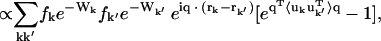 |
(2) |
where fk and rk are the scattering power and the mean position vector of the kth atom, respectively, uk is the displacement vector of atom k from rk, 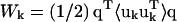 is the Debye-Waller factor, and 〈·〉 denotes the time or ensemble average. Equation 2 introduces the displacement variance-covariance matrix,
  . The displacements uk can be directly calculated from an MD trajectory and the variance-covariance matrix is then readily computed.
In the present work an improved version of the program SERENA (Micu and Smith, 1995) was used to calculate three-dimensional scattering intensities. These intensities were compared with experimental diffuse scattering data from the same crystal reported in Wall et al. (1997). In Wall et al. (1997), the Bragg peaks in the experimental scattering pattern were removed by an image filtering technique. The resulting three-dimensional experimental diffuse scattering pattern comprises 55,691 data points in the range ∥q∥ < 0.62 Å−1 and arises from the diffuse scattering of the complete unit cell, i.e., proteins and solvent.
The agreement between the theoretical and experimental x-ray diffuse scattering data was investigated using diffuse scattering calculated on several timescales, Δt, as described in Methods (Convergence of time series). The agreement factor, R, is defined as
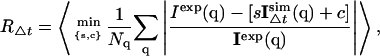 |
(3) |
where 〈·〉 denotes the average over all subtrajectories of length Δt, Nq is the number of scattering vectors, and s and c are coefficients for intensity scaling and background intensity, respectively.
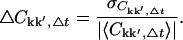
Correlation matrix
The variance-covariance matrix,  characterizes the protein collective motions. However, the large number of independent elements makes
  cumbersome to calculate for the whole unit cell. Here, the correlation matrix, Ckk′, for the relative displacements of all Cα-atoms in the unit cell was calculated instead, where Ckk′ is given by
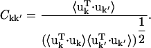 |
(4) |
For an atom pair (kk′) the correlation matrix element, Ckk′ is determined by the trace of the variance-covariance matrix, i.e., 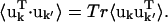 The differences between Ckk′ and
  are twofold. Firstly, anisotropic correlations, i.e., off-diagonal elements which describe correlations between the displacements in, e.g., the x and y directions, are not included in Ckk′. And secondly,
  is amplitude-weighted whereas Ckk′ is normalized. Alternative measures that overcome these problems are discussed in Héry et al. (1998). However, for the present purposes Ckk′ provides a convenient way of determining the correlated motions present.
Absolute values of Ckk′
There is no unique way of removing global rotation from MD trajectories (Hünenberger et al., 1995; Karplus and Ichiye, 1996; Abseher and Nilges, 1998; Zhou et al., 2000). Furthermore, MD algorithms that periodically remove global translation and rotation of the simulated system potentially introduce artifactual anticorrelations. To understand this, consider a one-dimensional system composed of two particles at positions x1(t) = 0 and x2(t) = x(t) where x(t) is an arbitrary displacement. Then Eq. 4 yields  . In the center-of-mass frame, however, is
  and
and  and hence
  .
.
To investigate the amplitude of the effect of removing global protein motion on Ckk′ we examined a 100-ps segment of the MD simulation T1 without the removal of global translation and rotation. The correlation coefficients, Ckk′ were directly computed from this trajectory segment using Eq. 4. Subsequently, global translation and rotation were removed and again Ckk′ was computed. Removal of global translation and rotation reduces the correlation coefficient by ∼−0.1 for intra- and interprotein motions almost independently of the interatomic distance (results not shown). Consequently, the average values of Ckk′ given in Figs. 4, 7, and 8 A are underestimated by ∼0.1.
FIGURE 4.

Displacement correlation matrix elements for all Cα-atoms plotted against their average distance, rkk′, for intraprotein motions (A) and interprotein motions (B). Both graphs were computed for the full trajectory T1 with length 10 ns. The shaded lines show the average values for distance intervals of width 1 Å. The atomic distance, rkk′, between two atoms k and k′, was calculated as rkk′ = min R{||rk − rk′ + R||}, where R is a lattice vector and thus rkk′ is the minimum distance between atom k and any crystal image of atom k′ created by the periodic boundary conditions.
FIGURE 7.

〈Ckk′, Δt〉 versus 〈rkk′〉 for atom pairs local or nonlocal in sequence. For the local-in-sequence data error bars are drawn along the principal axes of each (Ckk′, Δt, rkk′)Δ-distribution. The dotted line connects data points for atom pairs that are local in sequence. The inset shows the non-local-in-sequence data over the full distance range and shows a profile similar to Fig. 4 A. Results are shown for trajectory T2 with a subtrajectory length Δt = 1.0 ns. Error bars denote the standard deviation.
FIGURE 8.

(A) Pairs of Cα-atoms for which the protein-internal displacement correlations converged. The regions of secondary structural elements are indicated and their average correlation coefficients are given in parentheses. The results shown are for the merged trajectories Tx (x = 1+2+3) with subtrajectory length Δt = 2.5 ns. The gray-scale indicates the number of proteins for which Ckk′ converged. (B) Structure of Staphylococcal nuclease with secondary structural elements indicated.
Convergence of Ckk′
To study the convergence properties of Ckk′ each trajectory was divided into non-overlapping subtrajectories as described in Methods (Convergence of time series). For each subtrajectory the correlation matrix was computed. For each Δt, the correlation matrices for each subtrajectory were averaged elementwise to yield the mean, 〈Ckk′, Δt〉, and standard deviation,  The relative error, ΔCkk′, Δt, is then
 |
(5) |
For all quantities, the subscript Δt highlights the dependence on the length of the subtrajectories. The convergence criterion chosen was  where ∨ symbolizes the logical or. It was checked that the qualitative results do not depend on the specific choices of
  or ΔCkk′, Δt. If the number of subtrajectories is small (
 ) the statistics worsen, leading to an overestimation of the number of converged elements due to a small but non-zero probability that matrix elements coincidentally satisfy the convergence criterion. The amplitude of this effect was estimated using a corresponding number of random matrices. The true converged fraction of the correlation matrix,
  was then calculated as the difference
  where
where  and
and  were calculated from Ckk′ and the random matrices, respectively.
RESULTS
We first compare the MD simulation with experiment on three levels: the crystal parameters and average structure, the atomic fluctuations, and the x-ray diffuse scattering. Subsequently, correlations in Cα-atom motions are investigated.
Crystal parameters and average structure
The average values for the MD unit cell sides and volumes are given in Table 1. For the trajectories Tx (x = 1,2,3) and O1 these values deviate by less than 0.8% and 2.8% from the experimental values, respectively. The unit cell volume averaged over all simulations is within (0.35 ± 0.23)% of experiment.
TABLE 1.
The average values for the MD unit cell sides and volumes for the simulations (T1–3,O1) and the experimental values (Wall et al., 1997)
| a [Å] | b [Å] | c [Å] | V [Å3] | |
|---|---|---|---|---|
| Exp. | 48.5 | 48.5 | 63.4 | 149,132.65 |
| T1 | 48.3 ± 0.2 | 48.3 ± 0.2 | 63.8 ± 0.4 | 148,555 ± 419 |
| T2 | 48.6 ± 0.2 | 48.6 ± 0.2 | 63.0 ± 0.4 | 148,706 ± 413 |
| T3 | 48.6 ± 0.2 | 48.6 ± 0.2 | 62.9 ± 0.5 | 148,695 ± 392 |
| O1 | 49.9 ± 0.7 | 47.6 ± 0.3 | 62.6 ± 0.8 | 148,634 ± 399 |
To compare the simulation structure with the experimental coordinates (i.e., 2SNS) the average MD protein structure was computed as a time average  where RiTx(t) is the coordinate vector of protein i (i = 1, …, 4) in the simulation Tx. ⋃ denotes the union of sets which was performed in such a way that each RiTx(t) was optimally superposed (by minimizing the RMS deviation, or RMSD) on a reference structure (the single-protein mean structure). Thus, for certain analyses the trajectories Tx were merged into a single-protein trajectory with effective length of 120 ns. The RMSD of Rave from experiment was computed for the experimentally resolved residues 1–141. The result for all non-hydrogen atoms is 1.67 Å, and for the Cα-atoms is 1.29 Å.
Fluctuations of single atoms
X-ray crystallographic B-factors, Bk, arise from the fluctuations of the individual atoms k around their space-group symmetric positions as given by
 |
(6) |
The fluctuations may arise from internal protein motions, from translation and rotation of the protein molecules in the unit cell, and from motions of the unit cells relative to each other. Experimentally, other effects such as lattice distortion and refinement errors may also contribute. The relative motions of unit cells are suppressed in the simulations due to the imposition of periodic boundary conditions. Thus, the remaining fluctuations contain components from whole-molecule translation and rotation and from internal motion. The protein fluctuations were derived from the trajectories RiTx(t), x = 1,2,3, and the results are compared with the experimental B-factors in Fig. 1. The MD simulation fluctuations correlate well with those derived experimentally as supported by a correlation coefficient of 0.89. However, the MD fluctuations tend to be slightly larger, especially in the loop regions. Fig. 1 also shows that whole-molecule translations and rotations contribute ∼0.25 Å2 to the total MS fluctuations.
FIGURE 1.

Mean-square Cα-atom fluctuations calculated from the MD trajectories and from experiment. The simulation-derived fluctuations are: the total 〈uk2〉, including internal motion and whole-molecule translation and rotation (SIM: total); the total 〈uk2〉 with a Gaussian fit to the atomic positional distribution (SIM: Gaussian, see text); the contribution from internal motion (SIM: intra); and the contribution from whole-molecule translation and rotation (SIM: whole mol.). The decomposition of motions is described in detail in the text, see Eqs. 7 and 8. Experimental values were computed from B-factors using Eq. 6. B-factors were not reported in the starting structure used for the MD simulations (2SNS). Therefore, the experimental B-factors shown here are from 1STN (Hynes and Fox, 1991), a room-temperature structure refined at 1.7 Å with an R-factor of 0.162 and very similar unit cell parameters (a = b = 48.5 Å and c = 63.5 Å). Segments of secondary structures are indicated, see Fig. 8.
One possible reason why the simulation-derived fluctuations are slightly larger than experiment may be the assumption made in deriving the experimental B-factors that the fluctuations are harmonic. This assumption has been shown to lead to an underestimation of fluctuation magnitudes (García et al., 1997). To examine the consequences of this assumption, the fluctuations for each atom were recalculated from Gaussian fits to the simulation-derived atomic positional densities. The results, which correspond to the experimental isotropic B-factors, are presented in Fig. 1. Use of the Gaussian assumption does indeed significantly reduce the fluctuations, especially in the loop regions. However, the approximation does not account for most of the difference with experiment, the MD fluctuations remaining higher than experiment.
The atomic mean-square fluctuations can be decomposed as
 |
(7) |
 |
(8) |
where 〈uk2〉 is the total mean-square fluctuation of atom k, the displacements Iuk, Tuk, and Ruk describe the fluctuations due to the protein internal motion, whole-molecule translation, and whole-molecule rotation, respectively, and Kk represents correlations between the displacements Xuk, X = {I,T,R}. The mean-square fluctuations of the displacements Xuk were calculated from the MD trajectories as follows: to calculate Iuk a new trajectory was created in which the protein whole-molecule motion was removed by superposing all coordinate sets of a single-protein trajectory, Ri(t), on a single-protein reference structure (the mean structure of Ri(t)). To calculate the whole-molecule rigid-body displacements, Tuk and Ruk, a new trajectory was created by superposing the mean structure of Ri(t) on each coordinate set of Ri(t). For protein internal motions the mean-square fluctuation is  = 0.74 Å2. In comparison, whole-molecule translation contributes
  = 0.13 Å2 and the whole-molecule rotational contribution is
  = 0.16 Å2. The whole-molecule rotational contribution converged on the 1-ns timescale with an average molecule-rotation angle of (1.2 ± 0.1)°. The translational contribution converged more slowly, on the 10-ns timescale. Thus, the total mean-square fluctuation
  = 1.07 Å2 arises mostly (69%) from internal protein motion, with whole-molecule translation and rotation contributing equally to 27%. Although cross-correlations between the atomic displacements Xuk, 〈Kk〉k = 0.04 Å2 contribute only 3% of the mean-square fluctuations, their average magnitude 〈|Kk|〉k = 0.09 Å2 corresponds to 8% of the total fluctuations. This indicates that X = {I,T,R} is not an optimal basis for decomposition, due to the fact that, for a nonrigid body, the internal and whole-molecule motion cannot be strictly distinguished, leading to Kk ≠ 0.
A related question is whether the simulation-derived 〈Iuk2〉 values in Fig. 1 have converged. To examine this, the analysis scheme introduced in Methods was applied. The results for all simulations are quantitatively similar. Those for simulation T1 are depicted in Fig. 2. For the majority (∼65%) of atoms the fluctuations reach a plateau after 2–4 ns and the error bars gradually reduce during the progression of the simulation. This behavior is exemplified by  in the figure, which is situated in a turn between two β-strands. For a smaller fraction (∼15%) of atoms, however, the fluctuations significantly increase throughout the simulation, as exemplified in the figure by
  Most of these atoms are located either in a highly-flexible loop region (residues 46–51) or in the very mobile C-terminus that was not visible crystallographically (residues 142–149). As a result, due to this smaller fraction the fluctuation averaged over the whole molecule increases steadily with time. The fluctuations of the remaining 20% of atoms exhibit more complex behavior, one example being
  , which is situated in a coil region.
FIGURE 2.

Protein internal RMS fluctuations for all Cα-atoms averaged over subtrajectory lengths Δt (shaded lines) shown for a single protein of trajectory T1. Highlighted in black are the average overall Cα atoms and three examples of different time-dependence. Error bars denote the standard deviation. For clarity, only error bars for Cα29 are shown.
X-ray diffuse scattering
X-ray diffuse scattering is determined by the variance-covariance matrix, Eq. 2, and thus originates from cross-correlations in atomic displacements. Fig. 3 presents the time-dependence of the agreement factor, RΔt, between the simulation with the lowest R-factor (T3) and the experimental scattering data from Wall et al. (1997). RΔt reduces to ∼10% within the first 500 ps and then continues to decrease slowly on the nanosecond timescale, reaching 8.1% at 10 ns. The continued decrease of RΔt with time indicates that the scattering has not yet converged in the simulation but that the scattering intensity more closely resembles the experiment when the nanosecond-timescale dynamics are included. The dashed line shows the least-squares fit of  and demonstrates that the agreement factor decays logarithmically with time. Again, for all simulations, RΔt is similar. The R-factors and fit results from each simulation are given in Table 2.
FIGURE 3.

Dependence of the x-ray diffuse scattering agreement factor, RΔt on the averaging time interval Δt . The dashed line represents a least-squares fit (see text and Table 2). The figure shows results for the simulation T3. The results from the other simulations are very similar. Error bars denote the standard deviation.
TABLE 2.
Agreement factors RΔt=10 ns between the experimental diffuse x-ray pattern (Wall et al., 1997) and the scattering obtained from each trajectory
| RΔt=10 ns | A | B | Δt*R=0.00 | Δt*R=0.04 | |
|---|---|---|---|---|---|
| T1 | 8.15 | 9.90e-2 | −7.07e-3 | 1.2 ms | 4.2 μs |
| T2 | 8.35 | 9.91e-2 | −6.45e-3 | 4.8 ms | 9.6 μs |
| T3 | 8.08 | 9.81e-2 | −7.45e-3 | 0.52 ms | 2.4 μs |
| O1 | 8.56 | 9.86e-2 | −5.49e-3 | 63 ms | 43 μs |
A and B are results of least-squares fits (see text) and the remaining two columns give extrapolated convergence times Δt* for specified values of R.
Correlations in Cα-atom displacements
The B-factor results in Fig. 1 and the diffuse scattering R-factor plot in Fig. 3 suggest that the agreement with crystallographic experiment is sufficient to warrant a more probing analysis of the simulation data. To do this, the correlations in Cα-atom motion are now examined and related to the interatomic distances and protein topology. The convergence properties of the Cα displacement correlation matrix are also investigated.
In Fig. 4 are shown the displacement correlation matrix elements, Ckk′, for intra- and interprotein atom pairs, calculated for trajectory T1 and plotted against their corresponding interatomic distances, rkk′. The average values of Ckk′ as a function of rkk′ are indicated by the shaded lines. Intraprotein motions of atom pairs separated by less than ∼20 Å are mostly positively correlated. For larger atomic separations the values of Ckk′ range approximately from −0.5 to +0.5 for both distributions, i.e., for intra- and interprotein atom pairs. For rkk′ < 20 Å the intraprotein motions exhibit a significantly higher degree of correlation than motions between different proteins. At larger separations intra- and interprotein motions on average appear slightly anticorrelated. However, as described in Methods, this anticorrelation is an artifact due to the MD algorithm periodically removing the center-of-mass translation and rotation of the unit cell. Consequently, motions of atoms separated by  Å are uncorrelated.
We now investigate the convergence properties of Ckk′. To address this issue, the absolute and relative errors,  and ΔCkk′, Δt, respectively, were computed for non-overlapping subtrajectories with lengths Δt = 0.1, … , 5.0 ns and the converged fraction,
  was calculated as described in Methods. Only intraprotein motions showed a significant degree of convergence. Hence, only these correlations are discussed in the following. Fig. 5 presents the dependence of the intraprotein
  on Δt . Apart from in simulation T2, the converged fraction increases roughly logarithmically with Δt. Fig. 5 also shows that the degree of convergence varies significantly between the simulations. For the equivalent simulations Tx (x = 1,2,3) one finds fT2 > fT1 > fT3, indicating that simulation T2 possesses the highest degree of convergence. In contrast, Table 2 indicates that the agreement factors R display the reverse order, with simulation T3 in best agreement with experiment. This apparent conflict may be resolved by considering a simulation restricted to a region of phase space significantly smaller than that explored in the experiment. The variance-covariance matrix may appear to approach convergence in this simulation. If, then, the simulation crosses a free-energy barrier into another, previously unexplored region of phase space, then the variance-covariance matrix will appear to be far from convergence, whereas the elements themselves may resemble the experimental values more closely.
FIGURE 5.

Fractions of converged correlation matrix elements,  at different lengths, Δt of subtrajectories for all simulations, and two merged trajectories. Results are shown for intraprotein motions.
Also of interest is whether the matrix elements, Ckk′, converge to the same value in different simulations. This can be investigated by calculating  for the merged trajectories Tx and Tx + O1 (x = 1+2+3), respectively. If Ckk′ converges to the same value in all simulations, it contributes to
  ; otherwise, it does not. On the other hand, if Ckk′ does not converge in any single simulation then it is unlikely to converge in the merged trajectories. Therefore, the maximum value of
  for the merged trajectories is determined by the simulation with the lowest degree of convergence, i.e., T3.
  for the merged trajectories are also shown in Fig. 5. For Δt = 2.5 ns the convergence of Tx and Tx + O1 differ by 5% and 13% from T3, respectively. Thus, the majority (87%) of the converged matrix elements converged to the same value in all four simulations.
In Fig. 6 the intraprotein  is plotted against the interatomic distance, the fraction calculated from a random matrix,
  (see Methods), being negligible (9 ± 1)10−4. For shorter distances,
  6 Å, >80% of the intraprotein correlation matrix converges on the timescale of Δt = 1.0 ns. This fraction drops to ∼10% for rkk′ = 12 Å and becomes effectively zero for separations larger than 15 Å.
FIGURE 6.

Fraction of the intraprotein correlation matrix elements that has converged,  versus the atomic separation, rkk′. Results presented are for subtrajectory length Δt = 1.0 ns.
Also of interest is the dependence of the correlation matrix on the protein topology. To assess this, only converged elements of the intraprotein correlation matrix are examined. Due to the covalent bonding structure, one might expect the correlations between atoms local in the sequence to be larger than those between neighboring atoms which are nonlocal in sequence. The mean values, 〈Ckk′, Δt〉, for atom pairs that are local in sequence, defined here as Δ = |k – k′| < 10 (note that for Cα-atoms k and k′ are identical with the residue numbers), are compared in Fig. 7 with pairs that are nonlocal in sequence (Δ ≥ 10) as a function of 〈rkk′〉. Indeed, the displacement correlations between atoms that are local in sequence are on average larger than those between atoms that are nonlocal in sequence. The difference is ∼0.1, independent of 〈rkk′〉. Furthermore, the inset in Fig. 7 clearly demonstrates that the degree of correlation for nonlocal atoms decreases only slowly with increasing separation. Closely resembling the average distance-dependence for all matrix elements shown in Fig. 4 A, the magnitude of the converged elements decreases approximately exponentially with 〈rkk′〉 with a decay length of 10.6 Å for 〈rkk′〉 < 25 Å, beyond which 〈Ckk′〉 = 0.
Finally, we investigate where atoms, for which the intraprotein correlation matrix elements have converged, are located within the protein. In Fig. 8 A are shown the converged pairs of Cα-atoms in the simulations Tx (x = 1,2,3) with Δt = 2.5 ns. 94 percent of all nearest and 68% of all second-nearest backbone neighboring pairs converged in all four proteins in the unit cell. Most of the regions in which the correlations converged are located in secondary structural elements. The correlations between atoms located in α-helices converge for sequence distances Δ≲7. In contrast, the atom pairs within β-strands converge only for Δ≲ 2. The off-diagonal elements are converged atom pairs that are nonlocal in sequence. The majority of these are correlations between secondary structure elements. For almost all the strands in the Staphylococcal nuclease β-barrel the interstrand correlations have converged. Moreover, there is some convergence between α1 and α2, and pronounced convergence between α2 and α3. Correlations between the α- and β-elements in general have not converged. Finally, a comparison between Figs. 1 and 8 demonstrates that the converged correlations exist in regions of low mean-square fluctuation.
DISCUSSION AND CONCLUSIONS
Molecular dynamics simulations of crystalline Staphylococcal nuclease have been performed and analyzed in terms of B-factors, the atomic displacement correlation matrix, and x-ray diffuse scattering.
The average protein structures in all simulations are in accord with the experimental reference structure (1.3 Å average Cα RMSD). The unit cell edge parameters and volume are also well reproduced, indicating that protein packing is described correctly.
Isotropic B (thermal) factors are widely used to derive atomic fluctuations from x-ray crystallographic protein structures. The question arises, however, as to whether an unambiguous description of the dynamics involved can be derived from B-factor data in the absence of detailed additional information. B-factors contain static and dynamic components (Frauenfelder et al., 1979; Chong et al., 2001). Part of the static disorder may be temperature-independent. However, as the temperature of a protein is lowered some of the dynamic disorder may become static as proteins freeze into structurally inhomogeneous conformational substates. Separation of static from dynamic disorder is therefore nontrivial.
One approach is to fit simplified displacement models directly to the B-factor distribution. However, this approach suffers from the drawback that many such qualitatively-different models may yield fits of similar quality. Thus, it has been shown that a rigid-body translation/libration/screw (TLS) displacements model (Schomaker and Trueblood, 1968), in which the whole protein is considered as rigid and internal dynamics is absent, accurately reproduces most (Diamond, 1990) or all of protein B-factor distributions (Kuriyan and Weis, 1991). Alternatively, TLS models in which parts of the protein are considered rigid (e.g., aromatic side chains) have also been shown to successfully fit B-factor data (Howlin et al., 1989; Winn et al., 2001). An alternative model involves rigid-protein TLS degrees of freedom together with the internal dynamics described by normal mode eigenvectors with refinable amplitude factors (Diamond, 1990; Kidera and Gō, 1990; Joti et al., 2002). Moreover, a very simplified Gaussian vibrational model, in which the protein is described as an elastic network of locally interconnected Cα-atoms in the absence of whole-molecule motion, was also shown to produce B-factor distributions that agree very well with experiment (Tirion, 1996; Bahar et al., 1997; Kundu et al., 2002). Very recently, it has been demonstrated that B-factor distributions are closely correlated to local protein packing densities (Halle, 2002).
The availability of the above variety of fundamentally different models, all of which reproduce experiment, testifies to a lack of information that can be directly extracted from B-factor distributions. Thus, additional information must be supplied. For the dynamical contribution, this additional information is conveniently furnished by molecular simulation, in the form of the dynamical equations and the associated atomic model and force field. MD simulation offers a direct way of determining protein internal and whole-molecule motion (Hünenberger et al., 1995; Héry et al., 1998). However, due to computational limitations only part of the dynamics of the system is explored, i.e., in the present simulations of Staphylococcal nuclease, fluctuations are sampled occurring on the nanosecond timescale and on lengthscales shorter than the box size of the simulation, i.e., the unit cell. That longer timescale fluctuations exist, which are not sampled in the simulation, can be inferred from the present results. Furthermore, correlated motions between unit cells, such as commonly produce diffuse scattering streaks and rings associated with the reciprocal lattice, are also suppressed by the imposition of periodic boundary conditions.
Although in the simulations the fluctuations derived from the whole-molecule rigid-body external dynamics resemble the distribution of the total mean-square fluctuations, their contribution to the total mean-square fluctuations is significantly smaller than that from internal motions. Internal and whole-molecule motions were found to contribute ∼0.74 Å2 (69%) and ∼0.29 Å2 (27%) to the total mean-square fluctuations, respectively. Only in the regions of the secondary structural elements are both contributions of comparable magnitude. Furthermore, the present results indicate that the separation of the fluctuations into whole molecule translation, rotation, and internal motion does not provide an adequate basis for describing B-factors. Therefore, the TLS-model may not provide a physically consistent description if the protein is represented as a single rigid-body.
The simulation-derived total mean-square fluctuations are significantly larger than those derived from the experimental B-factors (cf. Fig. 1), as has been observed in previous MD studies (Hünenberger et al., 1995; García et al., 1997; Caves et al., 1998; Eastman et al., 1999). Although part of the difference with experiment is due to the harmonic assumption made in deriving the experimental B-factors, most of the difference has other origins. One possible contribution is the presence of crystallization agents, ligands and/or large-size ions, e.g., sulfate, in the experiment (which are absent in the simulation) which, due to steric hindrance and/or salt-bridges, could restrict protein motion. Also, the simulation setup and performance (e.g., the building of unresolved residues, length of equilibration) or inaccuracies of the force field, may have an influence. Furthermore, the uncertainties in experimental B-factors may be large. For example, the Cα mean-square fluctuations derived from 1SNM (Loll and Lattman, 1990), a Staphylococcal nuclease structure similar to 1STN, are on average 30% larger than those shown in Fig. 1.
A large fraction (∼65%) of the fluctuations converges on the nanosecond timescale. The nonconverged segments comprise the experimentally unresolved C-terminus region (residues 142–149), a highly flexible loop (residues 46–51), and some coil regions for which the fluctuations vary non-monotonically with the simulation length.
Additionally, the convergence properties of the atomic displacement cross-correlation matrix, Ckk′, have been determined here as a function of the length of the simulations. In molecular simulations, collective properties often converge on longer timescales than single-particle properties, and poor sampling of the displacement correlation matrix in protein MD has been previously noted (Clarage et al., 1995; Hünenberger et al., 1995). Here, it is found that parts of the protein-internal interatomic displacement correlation matrix converge on the nanosecond timescale whereas other parts do not. A crucial factor is the atomic separation. For atoms separated by ≲7 Å more than 50% of Ckk′ converge on the nanosecond timescale in the simulations. The magnitude of the converged matrix elements decays, on average, approximately exponentially with distance, with a decay length of 10.6 Å. Furthermore, convergence is seen between the strands comprising the β-barrel of the protein and between some neighboring α-helices, but not between the α- and β-regions of the protein.
For intraprotein motion, the converged fraction of Ckk′ grows logarithmically with the simulation length, cf. Fig. 5, a finding consistent with the logarithmic decay of the diffuse scattering R-factor with time (Fig. 3), which is determined by the convergence of the variance-covariance matrix. A physical model consistent with this logarithmic time-dependence is as follows. For the variance-covariance matrix to converge the system must fully sample the accessible protein energy landscape. For proteins, the energy landscape consists of multiple minima separated by a distribution of barrier heights (Frauenfelder et al., 1991, 1999). The number, NM, of minima sampled is a measure of the fraction of the energy landscape sampled and thus the degree of convergence of the variance-covariance matrix. The configurational sampling within a single minimum is very fast, whereas transition rates between minima are slower and depend exponentially on the barrier height ΔE, occurring with an average transition time, tT ∼ exp(ΔE/kBT). If the neighboring minima are of higher energy than the original minimum, the system will return to the original minimum within a time shorter than tT. Therefore, the sampling of neighboring minima will converge on a timescale tT given by the maximum barrier height crossed between the original and neighboring minima. The observation that the variance-covariance matrix converges on a logarithmic timescale therefore implies that NM increases proportionally to, or as a polynomial function of, the maximum barrier height crossed, i.e., NM ∼ ΔE ∼ log(t).
Finally, the present results allow us to estimate how long an MD simulation might have to be to fully sample the collective motions within crystalline proteins. The protein collective motions are described by the displacement variance-covariance matrix, which in turn determines the x-ray diffuse scattering. Hence, the comparison with x-ray diffuse scattering experiments enables us to estimate the simulation length required for the variance-covariance matrix to converge. Convergence of the diffuse scattering, and thus the variance-covariance matrix, can be defined as occurring when the agreement factor between simulation and experiment reaches RΔt ≤ ɛ, where ɛ accounts for systematic and experimental errors. The required simulation length depends on the choice of ɛ and the system size. Estimates for the convergence time Δt* are given in Table 2 for the entire Staphylococcal nuclease unit cell and two ɛ-values. For a realistic value of ɛ = 0.04 the convergence time is of the order 1 μs for the tetragonally constrained simulations, i.e., 100 times longer than the present simulations.
Acknowledgments
We gratefully acknowledge A. D. Gruia for providing Fig. 8 B, T. Becker, B. Costescu, V. Kurkal, D. Sengupta, A.L. Tournier, Prof. G.M. Ullmann and A.C. Vaiana for useful discussions and Prof. S. Gruner for providing the x-ray diffuse scattering intensities.
References
- Abseher, R., and M. Nilges. 1998. Are there non-trivial dynamics cross-correlations in proteins? J. Mol. Biol. 279:911–920. [DOI] [PubMed] [Google Scholar]
- Amadei, A., A. B. M. Linssen, and H. J. C. Berendsen. 1993. Essential dynamics of proteins. Proteins. 17:412–425. [DOI] [PubMed] [Google Scholar]
- Andersen, H. C. 1980. Molecular dynamics simulations at constant pressure and/or temperature. J. Chem. Phys. 72:2384–2393. [Google Scholar]
- Bahar, I., A. R. Atilgan, and B. Erman. 1997. Direct evaluation of thermal fluctuations in proteins using a single-parameter harmonic potential. Fold. Des. 2:173–181. [DOI] [PubMed] [Google Scholar]
- Benoit, J. P., and J. Doucet. 1995. Diffuse scattering in protein crystallography. Q. Rev. Biophys. 28:131–169. [DOI] [PubMed] [Google Scholar]
- Berman, H. M., J. Westbrook, Z. Feng, G. Gilliland, T. N. Bhat, H. Weissig, I. N. Shindyalov, and P. E. Bourne. 2000. The Protein Data Bank. Nucleic Acids Res. 28:235–242. [DOI] [PMC free article] [PubMed] [Google Scholar]
- Bossa, C., M. Anselmi, D. Roccatano, A. Amadei, B. Vallone, M. Brunori, and A. D. Nola. 2004. Extended molecular dynamics simulation of the carbon monoxide migration in sperm whale myoglobin. Biophys. J. 86:3855–3862. [DOI] [PMC free article] [PubMed] [Google Scholar]
- Brooks, B. R., R. E. Bruccoleri, B. D. Olafson, D. J. States, S. Swaminathan, and M. Karplus. 1983. CHARMM: a program for macromolecular energy, minimization, and dynamics calculations. J. Comput. Chem. 4:187–217. [Google Scholar]
- Caspar, D. L. D., J. Clarage, D. M. Salunke, and M. Clarage. 1988. Liquid-like movements in crystalline insulin. Nature. 332:659–662. [DOI] [PubMed] [Google Scholar]
- Caves, L. S. D., J. D. Evanseck, and M. Karplus. 1998. Locally accessible conformations of proteins: multiple molecular dynamics simulations of crambin. Protein Sci. 7:649–666. [DOI] [PMC free article] [PubMed] [Google Scholar]
- Chong, S. H., Y. Joti, A. Kidera, N. Gō, A. Ostermann, A. Gassmann, and F. Parak. 2001. Dynamical transition of myoglobin in a crystal: comparative studies of x-ray crystallography and Mössbauer spectroscopy. Eur. Biophys. J. 30:319–329. [DOI] [PubMed] [Google Scholar]
- Clarage, J. B., T. Romo, B. K. Andrews, B. M. Pettitt, and G. N. J. Phillips. 1995. A sampling problem in molecular dynamics simulations of macromolecules. Proc. Natl. Acad. Sci. USA. 92:3288–3292. [DOI] [PMC free article] [PubMed] [Google Scholar]
- Cochran, W. 1963. Lattice vibrations. Rep. Prog. Phys. 26:1–45. [Google Scholar]
- Daniel, R. M., R. V. Dunn, J. L. Finney, and J. C. Smith. 2003. The role of dynamics in enzyme activity. Annu. Rev. Biophys. Biomol. Struct. 32:69–92. [DOI] [PubMed] [Google Scholar]
- Diamond, R. 1990. On the use of normal modes in thermal parameter refinement: theory and application to the bovine pancreatic trypsin inhibitor. Acta Crystallogr. A. 46:425–435. [DOI] [PubMed] [Google Scholar]
- Eastman, P., M. Pellegrini, and S. Doniach. 1999. Protein flexibility in solution and in crystals. J. Chem. Phys. 110:10141–10152. [Google Scholar]
- Eastman, U., L. Perera, M. L. Berkowitz, T. Darden, H. Lee, and L. G. Pedersen. 1995. A smooth particle mesh Ewald method. J. Chem. Phys. 103:8577–8593. [Google Scholar]
- Faure, P., A. Micu, D. Perahia, J. Doucet, J. C. Smith, and J. P. Benoit. 1994. Correlated motions and x-ray diffuse scattering in lysozyme. Nat. Struct. Biol. 1:124–128. [DOI] [PubMed] [Google Scholar]
- Frauenfelder, H., G. A. Petsko, and D. Tsernoglou. 1979. Temperature-dependent x-ray diffraction as a probe of protein structural dynamics. Nature. 280:558–563. [DOI] [PubMed] [Google Scholar]
- Frauenfelder, H., S. G. Sligar, and P. G. Wolynes. 1991. The energy landscapes and motions of proteins. Science. 254:1598–1603. [DOI] [PubMed] [Google Scholar]
- Frauenfelder, H., P. G. Wolynes, and R. H. Austin. 1999. Biological physics. Rev. Mod. Phys. 71:419–430. [Google Scholar]
- Garcia, A. E., and G. Hummer. 1999. Conformational dynamics of cytochrome c: correlation to hydrogen exchange. Proteins. 36:175–191. [PubMed] [Google Scholar]
- Garcia, A. E., J. A. Krumhansl, and H. Frauenfelder. 1997. Variations on a theme by Debye and Waller: from simple crystals to proteins. Proteins. 29:153–160. [PubMed] [Google Scholar]
- Halle, B. 2002. Flexibility and packing in proteins. Proc. Natl. Acad. Sci. USA. 99:1274–1279. [DOI] [PMC free article] [PubMed] [Google Scholar]
- Héry, S., D. Genest, and J. C. Smith. 1998. Rigid-body motion and x-ray diffuse scattering in crystalline lysozyme. J. Mol. Biol. 279:303–318. [DOI] [PubMed] [Google Scholar]
- Hoover, W. G. 1985. Canonical dynamics: equilibrium phase-space distributions. Phys. Rev A. 31:1695–1697. [DOI] [PubMed] [Google Scholar]
- Howlin, B., D. S. Moss, and G. W. Harris. 1989. Segmented anisotropic refinement of bovine ribonuclease A by the application of the rigid-body TLS model. Acta Crystallogr. A. 45:851–861. [DOI] [PubMed] [Google Scholar]
- Hünenberger, P. H., A. E. Mark, and W. F. van Gunsteren. 1995. Fluctuation and cross-correlation analysis of protein motions observed in nanosecond molecular dynamics simulations. J. Mol. Biol. 252:492–503. [DOI] [PubMed] [Google Scholar]
- Hynes, T. R., and R. O. Fox. 1991. The crystal structure of staphylococcal nuclease refined at 1.7 Å resolution. Proteins. 10:92–105. [DOI] [PubMed] [Google Scholar]
- Ichiye, T., and M. Karplus. 1991. Collective motions in proteins: a covariance analysis of atomic fluctuations in molecular dynamics and normal mode simulations. Proteins. 11:205–217. [DOI] [PubMed] [Google Scholar]
- Jorgenson, W. L., J. Chandrasekhar, J. D. Madura, R. W. Impey, and M. L. Klein. 1983. Comparison of simple potential functions for simulating liquid water. J. Chem. Phys. 79:926–935. [Google Scholar]
- Joti, Y., M. Nakasako, A. Kidera, and N. Gō. 2002. Nonlinear temperature dependence of the crystal structure of lysozyme: correlation between coordinate shifts and thermal factors. Acta Crystallogr. D. 58:1421–1432. [DOI] [PubMed] [Google Scholar]
- Karplus, M., and T. Ichiye. 1996. Comment on a fluctuation and cross correlation analysis of protein motions observed in nanosecond molecular dynamics simulations. J. Mol. Biol. 263:120–122. [DOI] [PubMed] [Google Scholar]
- Kidera, A., and N. Gō. 1990. Refinement of protein dynamic structure: normal mode refinement. Proc. Natl. Acad. Sci. USA. 87:3718–3722. [DOI] [PMC free article] [PubMed] [Google Scholar]
- Kundu, S., J. S. Melton, D. C. Sorensen, and G. N. J. Phillips. 2002. Dynamics of proteins in crystals: comparison of experiment with simple models. Biophys. J. 83:723–732. [DOI] [PMC free article] [PubMed] [Google Scholar]
- Kuriyan, J., and W. I. Weis. 1991. Rigid protein motion as a model for crystallographic temperature factors. Proc. Natl. Acad. Sci. USA. 88:2773–2777. [DOI] [PMC free article] [PubMed] [Google Scholar]
- Legg, M. J. 1977. Protein crystallography: new approaches to x-ray data collection, direct space refinement and model building. PhD thesis. Texas Agricultural and Mechanical University, College Station, TX.
- Loll, P. J., and E. E. Lattman. 1990. Active site mutant Glu-43→Asp in staphylococcal nuclease displays nonlocal structural changes. Biophys. Chem. 29:6866–6873. [DOI] [PubMed] [Google Scholar]
- MacKerell, A. D., D. Bashford, M. Bellot, J. R. Dunbrack, R. L. Evenseck, M. J. Field, S. Fischer, J. Gao, H. Guo, S. Ha, D. Joseph, L. Kuchnir, et al. 1998. All-atom empirical potential for molecular modelling and dynamics studies of proteins. J. Phys. Chem. B. 102:3586–3616. [DOI] [PubMed] [Google Scholar]
- Micu, A. M., and J. C. Smith. 1995. SERENA: a program for calculating x-ray diffuse scattering intensities from molecular dynamics trajectories. Comput. Phys. Comm. 91:331–338. [Google Scholar]
- Nosé, S., and M. L. Klein. 1983. Constant pressure molecular dynamics for molecular systems. Mol. Phys. 50:1055–1076. [Google Scholar]
- Schomaker, V., and K. N. Trueblood. 1968. On the rigid-body motion of molecules in crystals. Acta Crystallogr. B. 24:63–76. [Google Scholar]
- Showalter, S. A., and K. B. Hall. 2002. A functional role for correlated motion in the N-terminal RNA-binding domain of human U1A protein. J. Mol. Biol. 322:533–542. [DOI] [PubMed] [Google Scholar]
- Tirion, M. M. 1996. Large amplitude elastic motions in proteins from a single-parameter, atomic analysis. Phys. Rev. Lett. 77:1905–1908. [DOI] [PubMed] [Google Scholar]
- Wall, M. E., S. E. Ealick, and S. M. Gruner. 1997. Three-dimensional diffuse x-ray scattering from crystals of staphylococcal nuclease. Proc. Natl. Acad. Sci. USA. 94:6180–6184. [DOI] [PMC free article] [PubMed] [Google Scholar]
- Waller, I. 1925. Theoretische Studien zur Interferenz-und Dispersion theorie der Rontgenstrahlen. Dissertation. Uppsala University, Uppsala, Sweden.
- Walser, R., P. H. Hünenberger, and W. F. van Gunsteren. 2002. Molecular dynamics simulations of a double unit cell in a protein crystal: volume relaxation at constant pressure and correlation of motions between two unit cells. Proteins. 48:327–340. [DOI] [PubMed] [Google Scholar]
- Winn, M. D., M. N. Isupov, and G. N. Murshudov. 2001. Use of TLS parameters to model anisotropic displacements in macromolecular refinement. Acta Crystallogr. D. 57:122–133. [DOI] [PubMed] [Google Scholar]
- Zachariasen, W. H. 1946. Theory of X-Ray Diffraction in Crystals. John Wiley & Sons, New York.
- Zhou, Y., M. Cook, and M. Karplus. 2000. Protein motions at zero-total angular momentum: the importance of long-range correlations. Biophys. J. 79:2902–2908. [DOI] [PMC free article] [PubMed] [Google Scholar]