Analysis of repeatability in spotted cDNA microarrays

Abstract

We report a strategy for analysis of data quality in cDNA microarrays based on the repeatability of repeatedly spotted clones. We describe how repeatability can be used to control data quality by developing adaptive filtering criteria for microarray data containing clones spotted in multiple spots. We have applied the method on five publicly available cDNA microarray data sets and one previously unpublished data set from our own laboratory. The results demonstrate the feasibility of the approach as a foundation for data filtering, and indicate a high degree of variation in data quality, both across the data sets and between arrays within data sets.

INTRODUCTION

Robotically spotted cDNA microarrays are increasingly applied in large-scale gene expression analyses. With this technology, gene expression is typically estimated as ratios between measured signal intensities from a target mRNA sample under investigation and signal intensities from a reference mRNA, represented as cDNA and labeled with different fluorescent dyes and co-hybridized to a microarray with spotted cDNA PCR product probes. The technology relies on several critical steps, including mRNA sample extraction, possibly amplification and labeling, PCR probe preparation, slide preparation, hybridization, laser scanning and image processing (1). Many of the processes involved are highly non-linear and difficult to calibrate (2). As a result, cDNA microarray measurements are often quite noisy, in particular measurements of low-abundance mRNA species. Consequently, data from cDNA microarrays are commonly pre-processed to identify and remove low quality measurements in order to enhance and ensure reliability of the estimated gene expression ratios. A common first step is to carry out a procedure in which individual array elements (spots) are ‘technically’ flagged. In this procedure, spots are investigated in order to identify and flag technically flawed spots, most commonly by manual investigation of array images but also by automated analysis of image files using software. Such spots are normally removed prior to any subsequent analyses.

The next pre-processing step is often to identify and remove array elements where the measured intensities (from both samples) are assumed to be indistinguishable from background noise (3,4). This step is commonly referred to as filtering. We denote by spot intensity the uncorrected foreground intensity of the spot. In one often-used scheme, the ratio of the measured spot intensity relative to the local background intensity is calculated and those spots where this ratio is smaller than some fixed constant, for instance 1.4 (4,5), are not considered well measured and subsequently removed. In other words, it is required that the spot intensity is ≥40% higher than the local background. A slight variation of this scheme is based on comparing the spot and background intensities by computing the difference of spot minus background. Then, spots where the background-corrected intensity is smaller than some other constant, for instance 100 or 200, are removed.

These and similar fixed-threshold approaches have at least two difficulties. First, it is not clear what is an appropriate value for the threshold, and a value of, for example, 1.4 times the background may be quite arbitrarily chosen. Exactly which value is appropriate as threshold depends on several factors and is likely to vary from one experimental setup to another. Secondly, the amount of random noise is likely to vary significantly from array to array, and a value of 1.4 times the background may be appropriate for one array, but too high or low for another, even if the same experimental setup is used. Clearly, if the value is too low, too many poor quality measurements will be used in the analyses, and if the value is too high, many ‘valid’ observations will be removed.

Here we present a systematic analysis of data quality based on measurements from repeatedly spotted probes leading towards an adaptive method for filtering putatively noisy array elements. We defined data quality as the repeatability of data from spots presumably containing the identical probes, as identified by IMAGE clone ID or GenBank accession number. We measured repeatability by calculating a statistical repeatability coefficient, the deviation between pairs of measurements from spots with the same probe, and the linear correlation coefficient. The analysis and filtering method is demonstrated on five publicly available data sets and one previously unpublished data set. In our analyses of logarithm base 2 transformed estimates of expression ratios, the results show a very high degree of variation in data quality, as measured by these statistics, both between data sets and between arrays within the data sets. The results also show that with respect to accommodating a consistent level of data quality, fixed-threshold filtering, such as filtering spots with intensity <1.4 times background intensity on all arrays, performed poorly. We demonstrate how the clone repeatability can be used to adapt thresholds for filtering criteria while focusing on data quality and maximization of the number of observations amenable for further analysis.

MATERIALS AND METHODS

Data

We downloaded five publicly available cDNA microarray data sets (4–8). In the following, we will refer to these data sets as ‘Mopo’ (6), ‘Mopo-clin’ (7), ‘Lymphoma’ (4), ‘NCI60’ (5) and ‘Prostate’ (8), respectively. Four of these five data sets had been analyzed by the authors using the ScanAlyze image analysis software, and we extracted raw data, such as spot and background intensities from both channels, and technical flags, from ScanAlyze output files by the use of custom perl-scripts. For the Prostate data set, spot and background intensities were not available, only what the authors termed ‘calibrated ratios’ and corresponding quality scores (8).

The sixth data set analyzed was obtained from our own laboratory at the Norwegian Radium Hospital and will be referred to as the ‘DNR’ data set. Image files were analyzed with the GenePix software and data were extracted with perl-scripts. Complete protocols for mRNA extraction, printing, scanning and image analysis are provided on our website (http://www.med.uio.no/dnr/microarray/english.html).

We focused the analyses on repeatability of logarithm base 2 transformations of the ratios of background-subtracted intensities of the target and background-subtracted intensities of the reference. In the ScanAlyze output files, the background-subtracted intensities of the channel 2 (target) signals and channel 1 (reference) signals are denoted CH2D and CH1D, respectively. We analyzed logarithms, base 2, of the normalized ratios (RAT2N) as exported from the ScanAlyze files, the calibrated ratios from the Prostate data and the ratios denoted ‘Ratio of Means’ in the GenePix export files.

Pre-processing

Two initial filtering steps were always applied prior to any analyses. First, all spots where the estimated spot intensity was below or equal to the estimated background signal intensity, in either channel, were removed. Spots that had been technically flagged were also removed.

Assessment of repeatability

For a given cDNA microarray data set, let d be the number of arrays (raw data files) and let n be the number of spots (array elements) on each array. Let n_m be the number of repeatedly spotted clones and let n_s be the total number of spots containing any repeatedly spotted clone. For each i = 1,…, n_m, let k_i be the number of spots where this clone has been spotted, thus:

When referring to a single array, the measured log ratio of a repeatedly spotted clone is then denoted y_ij, with clone i, and repeated spotting j (where j = 1, …, k_i). In the context of several arrays, we will use the notation y^(l)_ij to denote the measurement in array l, with l = 1,…, d.

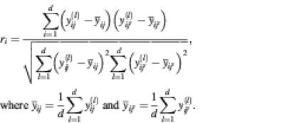
Correlation. For each clone, we calculated the average Pearson product-moment (linear) correlation between pairs of spots across data from the d arrays. If clone i has been spotted k_i times, there will be [k_i(k_i – 1)]/2 distinct pairs in its spot set. For a given pair of spots (denoted ij and ij′) we constructed the vectors [y^(l)_ij, …, y^(d)_ij] and [y^(l)_ij, …, y^(d)_ij], and computed the correlation coefficient with respect to clone i as

For a given clone, the correlation coefficient was calculated for all distinct pairs in the spot set, and the average correlation coefficient was used as an indicator of repeatability for the clone.

To assess the overall degree of repeatability in a whole data set in terms of correlation, we averaged correlation coefficients over all repeatedly spotted clones.

Mean absolute pairwise deviation. For each array we define the mean absolute pairwise deviation as the average absolute differences between measurements from paired spots (both containing the same clone). The average is taken over all clones and all distinct pairs in the spot set of each clone, that is,

where n′ is the number of terms in the sums.

Repeatability coefficient. As an indicator of the internal quality of a single microarray experiment we calculated a repeatability coefficient for each array (9). We defined the coefficient of repeatability as the value below which the difference between two measurements (log ratio) of a repeatedly spotted clone on the same array may be expected to lie with a probability of 95%. This coefficient was calculated for each array using analysis of variance (ANOVA) based on the spots from repeatedly spotted clones. As defined previously, let y_ij be the measured log ratio of repeatedly spotted clone i, where j = 1, …, k_i. For the ANOVA analysis we assumed each y_ij to be an independent realization of the variable Y_i ∼ N(µ_i, σ_i²). Furthermore, for each Y_i, i = 1, …, n_m, we assumed the σ_i to be identical and equal to (a common) σ. The repeatability coefficient was then defined as 2.83 × , where is as estimated from the sum of squared residuals through

Similarly, we calculated repeatability coefficients for clones across arrays. In this calculation, the arrays are viewed as effects and is, for a fixed i, estimated by

Note that in the data sets analyzed, k_i is fixed for each clone across all arrays in a set. This is not a limitation of the method and the computations can be adapted to allow for variable numbers of spots for a given clone across the arrays analyzed.

Adaptive filtering of weak spots

Under the assumptions that the variation in log ratio between spots containing the same probe at different levels of signal intensities is (i) indicative of quality of the data and (ii) representative for all measurements on the array with similar signal intensities, we defined a method to adapt the filtering thresholds to accommodate a fixed level of data quality.

We describe the method as applied to filtering based on the ratio of spot intensity over background intensity (SB ratio), but we emphasize that the method can be applied to any ‘measure of quality’ one would define as a filtering criterion. Possible choices of filtering criteria could be other versions of signal-to-noise criteria, e.g. the (spot intensity – background intensity)/(spot intensity), or more complex criteria such as the composite quality score presented by Wang et al. (10). We also tested the method with the difference of spot intensity minus background intensity (SB difference).

For each spot containing any probe that had been repeated, we calculated the selected filtering criterion (SB ratio) for both channels. The two channels were analyzed separately. For each channel, the values for the filtering criterion were then sorted and evaluated as possible candidates for the filtering threshold. For each possible filtering threshold, we calculated the estimated repeatability standard deviation based on the filtered data. We then compared the estimated repeatability standard deviation with a chosen target value σ₀. We defined the threshold for filtering as the smallest value at which the estimated repeatability standard deviation was below σ₀.

We chose the threshold for the estimated repeatability standard deviation to be σ₀ = 0.43 based on the following reasoning. A log 2 difference of 1 corresponds to a 2-fold change, and we believed this is a reasonable criterion for repeatability of spots containing the same clone. For data of good quality we would thus like the difference between the log ratio of a pair of spots from the same clone to be inside the interval [–1,1]. In our setting, this amounts to choosing σ₀ = 0.43, since the interval [–1,1] equals a 90% confidence interval of the difference between two realizations of an N(µ_i, σ²₀ random variable.

As the two channels would normally define differing cut-off values for filtering, we chose to handle this conservatively, i.e. to discard ratio data for all observations where the measurement from at least one channel was below the threshold value for this channel. As a visual aid for interpreting the filtering procedure based on the repeatability statistics, we plotted differences of log ratios from pairs containing the same clone versus the minimum (over the two spots in a pair) ratio of spot intensity over background intensity. From these plots we identified the threshold where 90% of the differences were smaller than 1 (in absolute value).

RESULTS

The first five data sets selected for analysis were chosen because they represented large publicly available data sets of human origin with a general clinical relevance. These five data sets originate from high-profile publications and are thus likely to represent state-of-the-art cDNA microarray technology. The data sets represented different laboratories, thus reflecting varying laboratory and analysis procedures. The procedural variation was considered beneficial, as it was expected to reflect general methodological variation inherent in the technological platform of spotted cDNA microarrays. The last data set was taken from our own laboratory at the Norwegian Radium Hospital (DNR) and was selected for comparison as part of developing a quality control effort in our own microarray production and analysis facilities.

The data sets represented a wide range in the total number of data points and printing patterns (Table 1). We calculated the number of spots that would be removed according to often-used filter criteria (Table 2). These numbers do not directly relate to the data quality, but nevertheless indicate that there is considerable variation in the relative levels of signal-to-background between the data sets.

Table 1. Summary descriptive statistics for the selected data sets.

	Number of arrays	Number of array elements (n)	Number of unique clones	Number repeatedly spotted (nm)	Number of spots, repeatedly spotted clones (ns)
Mopo	83	9216	8830	189	387
Mopo-clin	29	9216	8733	99	198
Lymphoma	67	18 432	14 181	2832	6759
NCI60	63	10 000	9703	3	6
Prostate	25	6500	6500	116	233
DNR	4	11 552	9377	1496	2992

From three publications (4,5,7) we extracted data from subsets of the arrays publicly available. This was because differing array print formats had been used, and we chose to use only the largest subset of identically printed arrays in order to ensure data integrity. The columns ‘Number of array elements’, ‘Number repeatedly spotted’ and ‘Number of spots, repeatedly spotted clones’, correspond to the numbers n, n_m and n_s, as defined in the Materials and Methods.

Table 2. Filtering statistics as given with common filtering rules.

	Total number of spots	% flags	% spot < background	% spot <1.4 × background	% spot <100 + background
Mopo	774 144	8.00	3.12 (2.53)	18.02 (15.26)	10.43 (8.84)
Mopo-clin	267 264	10.91	15.95 (12.10)	58.62 (48.80)	50.74 (41.67)
Lymphoma	1 234 944	1.20	2.45 (2.28)	33.42 (32.81)	47.66 (47.06)
NCI60	630 000	0.25	5.68 (5.66)	43.41 (43.28)	17.92 (17.88)
Prostate	162 500	NA	NA	NA	NA
DNR	46 208	31.91	3.41 (0.72)	7.15 (0.06)	45.36 (16.25)

The column ‘Total number of spots’ shows the total number of spots summed over all arrays from each data set. The ‘% flags’ column shows the percentage of spots that had been flagged, manually or by image analysis software, for each data set. The remaining columns show the total percentage of spots that would be removed according to common filtering criteria. For each of these columns, the main number shows the percentage when flagged spots are disregarded in the total number of spots, while the corresponding numbers in parentheses show the percentage of the number of spots also including the spots that were flagged. NA, data not available. The very high number of flagged spots in the DNR data set was due to a flagging procedure included in the GenePix image analysis software.

Global assessment of repeatedly spotted clones

Using the spots of clones that had been spotted in several positions on an array, we investigated the repeatability of the data sets. We calculated correlations for paired spot observations (as described in Materials and Methods) for each pair of each clone across all arrays, and averaged the correlations across the pairs to obtain a correlation for each clone. For each data set, the clone correlations were subsequently averaged to obtain an indicator of repeatability (Table 3). The Lymphoma data set appeared to have considerably higher repeatability in terms of average correlation than the other data sets.

Table 3. Correlation coefficient, mean absolute pairwise deviation, and repeatability statistics, σ for clones across arrays.

	Correlation coefficient		Mean absolute pairwise deviation		Repeatability statistic, σ
	All	Filtered	All	Filtered	All	Filtered
Mopo	0.646 (0.334)	0.676 (0.347)	0.598 (0.425)	0.510 (0.389)	0.588 (0.355)	0.470 (0.310)
Mopo-clin	0.527 (0.398)	0.634 (0.469)	0.929 (0.629)	0.565 (0.343)	0.855 (0.507)	0.539 (0.359)
Lymphoma	0.714 (0.269)	0.777 (0.397)	0.519 (0.317)	0.366 (0.222)	0.518 (0.294)	0.335 (0.200)
NCI60	0.429 (0.285)	0.515 (0.686)	1.159 (0.277)	0.558 (0.635)	1.101 (0.223)	0.463 (0.538)
Prostate	0.293 (0.342)	NA	0.615 (0.313)	NA	0.580 (0.313)	NA
DNR	0.592 (0.628)	0.593 (0.627)	0.900 (1.038)	0.899 (1.038)	0.901 (0.746)	0.889 (0.758)

The numbers are average values with standard errors in parentheses. For correlation coefficients, a clone average, across correlation coefficients from all pairs for the clone, was first calculated before a non-weighted average and standard error across clones was calculated for each data set. The mean absolute pairwise deviation was calculated as the average across all combinations of same-clone spot-pair and array within each data set. The ‘Repeatability statistic, ’ column shows the average for each data set of estimates of the standard deviations in the ANOVA model calculated for each repeatedly spotted clone (high quality corresponds with a small value for the repeatability coefficient). For each statistic, the value as calculated from all available data points (excluding spots that were below background or manually flagged) as well as the value calculated from the ‘standard’ filter-criterion of SB ratio ≥1.4, are given in columns ‘All’ and ‘Filtered’, respectively. The repeatability coefficient (as defined in the Materials and Methods) can be obtained from the estimated standard deviations by multiplying the repeatability statistics by 2.83. The corresponding standard error can also be found by scaling with the same factor.

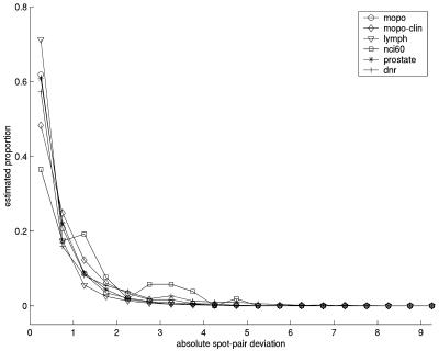
Although correlation coefficients have a straightforward interpretation, they may sometimes be misleading (9). We therefore also calculated the average absolute deviations (absolute value of the difference between spot 1 and spot 2) between measurements from paired spots (both containing the same clone), as well as a repeatability coefficient. Both of these indicators agreed well with the correlation coefficients when investigating clone by clone, i.e. that clones with high correlation across arrays also had smaller average deviations and smaller repeatability coefficients (data not shown). Except for the Prostate data set, the deviations and repeatability coefficients were also in agreement with the correlation coefficients when viewed globally for each data set (Table 3). The Prostate data set illustrated one of the points made by Altman and Bland (9), namely that a low correlation does not necessarily mean that the agreement between two data series is bad; the correlation tends to give a low estimate of agreement if there is little overall variation in the data. Although all data sets contained intra-clone spot pairs where the difference in log ratio between the two spots was as high as 8 or more, the distributions of spot-pair deviations were different (Fig. 1). For instance, in the Lymphoma data set, 87.5% of all pairwise absolute deviations were <1 (in absolute value), whereas for the Mopo-clin and DNR data sets the corresponding percentages were ∼73%.

Figure 1.

Plot showing the proportion of observations inside fixed-width intervals of intra-clone spot-pair deviations for the data sets mopo (circles), mopo-clin (diamonds), lymphoma (triangles), nci60 (squares), prostate (asterisks) and dnr (plus symbols). The deviations are based on log base 2 ratios and are calculated from all spots that had not been flagged and contained positive background-corrected spot intensities in both channels. The plot summarizes the information from separate histograms for each data set. The values on the vertical axis give the proportion of the data sets (range 0–1) present in the interval, and the values on the horizontal axis are the midpoints of the intervals. The intervals are 0–0.5, 0.5–1, …, 9.5–10. Values equal to the lower limit of each interval are included. Values equal to the upper limit of each interval are not included.

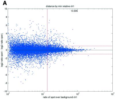
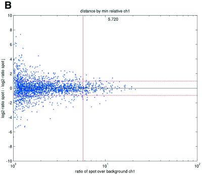
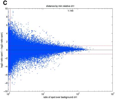
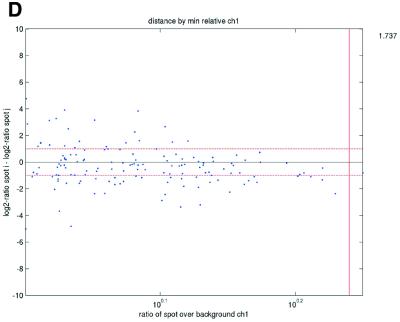
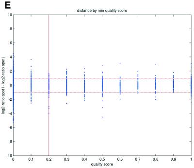
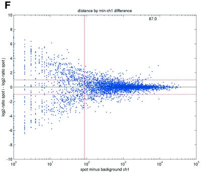
Previous studies have indicated that reliable measurements are more difficult to obtain for low-abundance than for high-abundance transcripts (11). In terms of signal intensities, this suggests that lower intensity measurements may be suspected to be less reliable than higher measurements. In terms of repeatability, a similar pattern was also observed in the data sets in the present study (Fig. 2). We consistently found that repeatedly printed spots with high signal intensities gave good repeatability, while the quality deteriorated as spot intensities approached the background signal levels. Plots of deviations between pairs of repeatedly spotted clones, pooled across arrays in each data set, versus both the ratios and differences between spot intensities and background intensities (minimum over the two spots in a pair) showed that the highest absolute deviations were found when the ratios or differences were low (Fig. 2).

Figure 2.

(Opposite) Spot-pair differences versus quality index. For each distinct pair of spots containing the same clone, the difference of log base 2 transformed gene expression ratio in the two spots was calculated. A quality index was calculated for each spot and the minimum over two spots in a pair was used to represent the pair. The plots show all pair differences versus (minimum) quality pooled over all arrays from each data set. For the ScanAlyze data sets mopo (A), mopo-clin (B), lymphoma (C) and NCI60 (D) we show the differences plotted versus the SB ratio calculated from channel 1 for each spot. For the prostate (E) data set, the spot quality index was provided by the authors. For the DNR (F) data set we show the differences plotted versus the SB difference calculated from channel 1 for each spot. Data for channel 2 are not shown, as the data are comparable with the respective channel 1 plots. Note that the x-axes are not on the same scale. The horizontal dashed lines are at –1 and 1, showing the limits for 2-fold difference in expression ratios between two spots in the same pair. The vertical lines are placed at the x-value which would result in 95% of the differences lying between –1 and 1 if used as a filtering criterion (by removing all data points to the left). Note that the NCI60 dataset had very few repeatedly spotted clones and that the quality index provided with the Prostate dataset only had discrete values with steps of 0.1 in the range 0–1.

Local assessment of repeatedly spotted clones

When investigating data quality locally on each array, we found considerable variation in repeatability across arrays within each data set (Table 4). This was also evident when investigating deviations of intra-clone spot pairs on each array. From Table 4, it is clear that the often-used filtering criterion of removing spots where the SB ratio was <1.4 provided a considerable improvement in repeatability compared with no filtering. However, the variation in repeatability between different data sets indicates that this common criterion was not equally appropriate for all experimental setups. In particular, the results suggested that the 1.4 criterion was far too low for the DNR data set, where only 0.06% of the spots not flagged would be filtered. The variation within data sets further indicates that there were varying levels of noise in different arrays from the same data set—motivating slide-individual adaptation of the filtering criterion.

Table 4. Repeatability statistics, σ, as calculated for arrays over repeatedly spotted clones.

	All applicable	Standard filtering
Mopo	0.674 (0.145)	0.548 (0.087)
Mopo-clin	0.885 (0.133)	0.504 (0.127)
Lymphoma	0.569 (0.120)	0.320 (0.058)
NCI60	0.974 (0.642)	0.632 (0.496)
Prostate	0.621 (0.217)	NA
DNR	1.131 (0.335)	0.917 (0.113)

The numbers are average values of the estimated standard deviations in the ANOVA model, as averaged within each data set across all array slides in that data set. The corresponding number in parentheses shows the standard error, as calculated from all array slides in the corresponding data set. The ‘All applicable’ column shows data as calculated from all data points with spot above background and not technically flagged. In the ‘Standard filtering’ column, data shown are as calculated from all data points where SB ratio ≥1.4. As in Table 3, the repeatability coefficient can be found by multiplying by 2.83. NA, data not available.

Adaptive filtering with control of data quality

Visual inspection of plots of the intra-clone spot-pair deviations versus the (minimum over the two spots in the pair) spot intensities may suggest sensible thresholds for the minimum spot intensity required for the repeatability to be acceptable (Fig. 2). However, we preferred to use the repeatability statistics to computationally determine the threshold (see Materials and Methods). By this method we found filtering thresholds for the spot intensity relative to the background intensity, both when comparing by ratios and by differences.

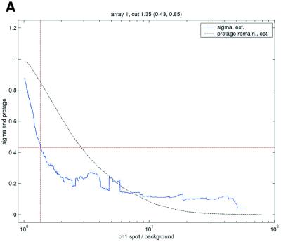
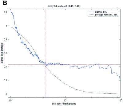
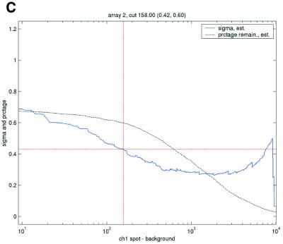
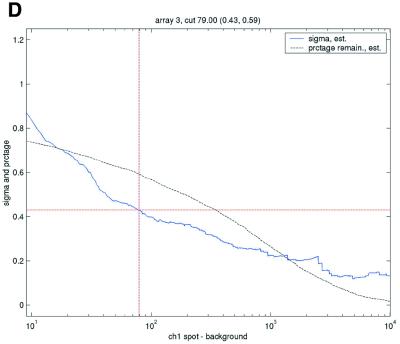
Enforcing a common level of data quality resulted in a highly varying level of filtering between the different arrays and data sets (Table 5). This was seen most directly in the number of data points filtered as not meeting the array-specific criterion. Given the repeatability statistics calculated from the 1.4 times background criterion, it was expected that the filtering thresholds for the SB ratio would generally be >1.4, except in the case of the Lymphoma data set. The array-specific thresholds found varied highly but are not as straightforward to compare across data sets. Illustrations of the variation in repeatability coefficient for different possible filtering values are shown in Figure 3.

Table 5. Adaptive determination of threshold for spot intensity relative to background intensity.

	Number of spots applicable	% remaining	Threshold
			ch1	ch2
Mopo	684 331	19.9	15.62 (13.60)	10.53 (12.98)
Mopo-clin	171 285	14.5	3.98 (3.07)	4.13 (3.52)
Lymphoma	1 119 833	70.2	1.83 (1.36)	1.30 (0.15)
DNR	29 836	66.4	113 (35.4)	335 (117.8)

The ‘Number of spots applicable’ column shows the total number of spots applicable to filtering in each data set. The ‘% remaining’ column shows the percentage of applicable spots that met the array specific quality-filtering criteria. For the DNR data set we found the spot minus background difference to be more useful than the SB ratio as a ‘quality-index’ to use for filtering. For the other data sets, data shown are for filtering based on the SB ratio. The ‘Threshold’ columns show the averages and the standard errors, in parentheses, of the array-specific filtering thresholds found for each data set and each channel.

Figure 3.

Filtering thresholds from quality-based filtering. Estimates of the standard deviation, , in the ANOVA model were obtained from all points strictly to the right of each possible cut-off value on the x-axes (solid lines). To adapt filter cut-off values we sought the smallest x-value giving rise to smaller or equal to a target value of 0.43. The vertical dashed lines are placed at the respective thresholds on the x-axes, corresponding to the cut-value shown in the plot-title. The horizontal dashed lines (red) are placed at y = 0.43, corresponding to the σ₀ used in the test. The solid (blue, ‘sigma, est.’) lines show the estimated values of sigma for each possible cut-off along the x-axis. The dashed (black, ‘prctage remain., est.’) lines show the estimated percentage of points that would remain when filtering at a given cut-off along the x-axis. Plots are shown for channel 1 data from arrays 1 and 34 in the Lymphoma data set. In this data set, array 1 was one of the better arrays in terms of data quality. The desired level of repeatability was attained with a threshold value at 1.28 for the SB ratio (in channel 1), whereas for array 34 the corresponding cut-off was found at 4.40. From the DNR data, channel 1 data for arrays 2 and 3 are shown in plots (C) and (D), respectively. As can be seen from these plots, the estimated cut-off values for filtering was much higher in array 2 than in array 3. (A) Lymphoma, array 1, channel 1, SB ratio. (B) Lymphoma, array 34, channel 1, SB ratio. (C) DNR, array 2, channel 1, SB difference. (D) DNR, array 3, channel 1, SB difference.

DISCUSSION

Information from repeatedly spotted clones is a valuable resource for data quality evaluation and control. An underlying line of thought is that several observations of the same quantity, under similar conditions, should be similar, and are more reliable than a single observation. Otherwise the observations contain pertinent information about the quality of the data. This is one of the rationales behind experiment replication (12,13). Replication goes some way in improving microarray data quality, but it may be objected that it is a not very cost-effective procedure and that the distribution of noise is far from random, frequently rendering the same observations problematic across replications. In comparison to experiment (array) replication, the experimental conditions relating to sample preparation, hybridization and scanning are much more similar for two spots on the same array. We consider experiment replication as a necessary strategy for assessing reproducibility that is complementary to internal duplication of spots. Moreover, we argue that reproducibility across identical arrays can be evaluated within our framework of repeatability of repeatedly spotted clones.

Internal duplication of spots has been applied in order to obtain more reliable estimates of expression ratios. Tseng et al. (14) used repeatedly spotted genes to remove all observations of each poor quality gene from the data. For each repeatedly spotted gene, they calculated the mean and standard deviation of the observed ratios of the gene (in their presentation each gene was spotted four times). A quality index for each gene was defined as the calculated standard deviation divided by the calculated mean of the ratios. Genes with a large value of the quality index were removed from the data. A cut-off value was defined dependent on the mean average signal in both channels. For each gene they found the 50 genes whose mean intensity (average of signal in both channels) were closest to the mean intensity of the selected gene. For all 50 genes the quality index was calculated and the cut-off value was defined as the 90th percentile of these quality indices (i.e. 10% of the quality indices are larger than the cut-off value). This strategy bears resemblance to ours in that both consider the variability of repeatedly spotted clones, but they differ in the following aspects. Tseng et al. (14) calculate the variability for each repeatedly spotted gene, requiring a larger number of multiple spots than our strategy, where the variability is calculated from all repeatedly spotted genes together. Further, their strategy for removal of spots requires removal of all spots from selected bad quality genes, and cannot be applied to genes that are not repeatedly spotted.

A necessary prerequisite to apply our method is that the number of repeated spots present on the arrays is sufficient for robust data analysis to be performed. As illustrated by the data sets used in this study, repeatedly spotted clones are common in array designs. In this case, elimination of multiples is less cost effective than retaining copies. Figure 1 shows that there is a clear relationship between intraclone spot-pair deviation and signal intensities, permitting our analytical approach. However, these values are based on probes naturally spotted in repeats when plates with PCR products from different cDNA libraries are printed on the same array. Indeed, there are significant contributions to variation, notably PCR product and pin variation, that are not accounted for in this analysis; this information was not available with the data sets analyzed. Thus, the variance of repeatedly spotted clones with the data sets used most likely represents an overestimation, and filtering criteria may need to be relaxed to counter this effect. To eliminate this problem, slides should be deliberately designed to include a subset of clones with repeatedly spotted clones from identical PCR products and with identical pins. We think that slides including such repeated spots would provide a very useful tool for many aspects of quality control and comparison. With respect to serving as a foundation for intensity-based filtering strategies, the set of repeatedly spotted probe sequences should include probes whose target mRNAs have a wide range of abundance. The approach can be generalized to encompass other sets of repeatedly spotted probes that can be safely assumed to give identical measurements. For instance, if one makes the (perhaps rather strong) assumption that distinct probes from the same gene should give the same measurement, it would be possible to use all spots representing the same gene. The optimal spot design remains to be decided, such as the optimal number of repeats per probe, the positioning of repeated spots, and the distribution of expected abundances across a wide range of mRNA samples. There is clearly a trade-off between increasing the number of copies per clone and the desire to measure as many genes as possible. However, we argue that internal duplication of spots is a viable approach to microarray data quality control that represents little added cost compared with other strategies.

Analysis of repeatability using repeatedly spotted probes gives a very direct estimate of data quality. In our study, we observed what appeared to be systematic differences in quality between different experimental setups. This may be a reflection of a number of technical issues inherent to the technology, such as defining optimal RNA extraction procedures, labeling and hybridization techniques, as well as printing, scanning and data handling variations. In order for microarrays to be widely accepted in clinical and diagnostic use, having high requirements to the precision and reliability of measurements, it appears that time is well spent optimizing technical parameters to maximize the amount of biologically relevant information.

When interpreting the results from this study, it is important to keep in mind that the different data sets had highly differing numbers of spots with at least one other copy; ranging from 6759 in the Lymphoma data set to 198 in the Mopo-clin data set, disregarding the NCI data set. Although the 99 clones spotted twice in the Mopo-clin data are likely to be sufficient to obtain a description of data quality, it could be argued that this may not be a sufficiently high number to serve as a foundation for filtering. For instance, in the Mopo-clin data set we identified a handful of repeatedly spotted clones that consistently had poor repeatability (data not shown); a similar and partly overlapping set of consistently poorly repeatable clones was identified in the Mopo data set. Clearly, such clones will systematically bias the filtering procedure and result in overestimated values for the filtering thresholds. When clones that consistently are poorly measured can be identified, the filtering procedure should be carried out after an initial step of removing the corresponding spots from the data set.

Several issues remain to be resolved with respect to microarray data filtering. One of the most central questions is how to determine the best discriminating ‘quality-criterion’ to use. This subject has not been resolved in this report. Several criteria other than the ones investigated in this report can be defined (10,15). Wang et al. (10) defined a composite quality score for each spot by multiplying quality scores of spot size, spot signal-to-noise ratio, local background variability and spot saturation. To use the composite quality score for filtering, a cut-off value must be set. Wang et al. (10) instruct the reader to set a cut-off value (values of 0.3, 0.5 and 0.85 are mentioned in the text). Our repeatability coefficient can be used to set array-dependent cut-offs for this composite quality score.

However, based on a statistically sound method for measuring data quality, filtering criteria can be evaluated by their ability to separate high quality measurements from poor quality measurements. In this respect, repeatability of measurements from repeatedly spotted clones should provide a sound framework for evaluating filtering criteria.

With any filtering procedure there is a trade-off between optimizing measurement reliability and avoiding loss of information. This should also be kept in mind when adapting a filtering criterion to ensure a given level of repeatability. For some studies, for instance if it is known that the mRNA sample(s) are of uncertain quality and when the duplicate observations of the same clone are based on different PCR products (and are thus not identical replicates), the cut-off value of σ₀ = 0.43 used in this study may be too strict and it may be more reasonable to relax these parameters and accept the risk of including more noisy data. We have chosen a cut-off value of σ₀ = 0.43 to be used for all microarrays, assuming that repeated clones differing more than 2-fold in ratio are undesirable regardless of the dynamic range of the log ratios on the microarray. We are investigating a repeatability measure that, in addition to the variability within clones (intraclone variability), also includes the variability between clones.

A possible further use of our method is to evaluate the relative merits of various normalization and calibration methods. Assuming that higher repeatability will be observed with better estimates of log ratios, or any other estimate of gene expression of interest, this approach can be used to compare and optimize various normalization and calibration methods, as better repeatability would be expected with an improved normalization procedure. Under similar assumptions, the framework can also be used to evaluate and optimize other parts of the cDNA microarray pipeline, ranging from methods for RNA extraction to various strategies for defining the background intensity estimates.

The optimal validation of our method would be to demonstrate biological significance when using our filtering procedure. Due to the absence of objective criteria, and the required detailed biological knowledge of a given data set, this falls outside the scope of the present paper. In any case, our method provides a general strategy to obtain objective quality measurements across slides and experiments, and to ensure homogenous data quality by adjusting filtering criteria adaptively.

REFERENCES

- 1.Schuchhardt J., Beule,D., Malik,A., Wolski,E., Eickhoff,H., Lehrach,H. and Herzel,H. (2000) Normalization strategies for cDNA microarrays. Nucleic Acids Res., 28, e47. [DOI] [PMC free article] [PubMed] [Google Scholar]
- 2.Yang Y.H., Dudoit,S., Luu,P. and Speed,T.P. (2001) Normalization for cDNA Microarray Data. SPIE BiOS, San Jose, CA.
- 3.Marton M.J., DeRisi,J.L., Bennett,H.A., Iyer,V.R., Meyer,M.R., Roberts,C.J., Stoughton,R., Burchard,J., Slade,D., Dai,H. et al. (1998) Drug target validation and identification of secondary drug target effects using DNA microarrays. Nature Med., 4, 1293–1301. [DOI] [PubMed] [Google Scholar]
- 4.Alizadeh A.A., Eisen,M.B., Davis,R.E., Ma,C., Lossos,I.S., Rosenwald,A., Boldrick,J.C., Sabet,H., Tran,T., Yu,X. et al. (2000) Distinct types of diffuse large B-cell lymphoma identified by gene expression profiling. Nature, 403, 503–511. [DOI] [PubMed] [Google Scholar]
- 5.Ross D.T., Scherf,U., Eisen,M.B., Perou,C.M., Rees,C., Spellman,P., Iyer,V., Jeffrey,S.S., Van de Rijn,M., Waltham,M. et al. (2000) Systematic variation in gene expression patterns in human cancer cell lines. Nature Genet., 24, 227–235. [DOI] [PubMed] [Google Scholar]
- 6.Perou C.M., Sorlie,T., Eisen,M.B., van de Rijn,M., Jeffrey,S.S., Rees,C.A., Pollack,J.R., Ross,D.T., Johnsen,H., Akslen,L.A. et al. (2000) Molecular portraits of human breast tumours. Nature, 406, 747–752. [DOI] [PubMed] [Google Scholar]
- 7.Sorlie T., Perou,C.M., Tibshirani,R., Aas,T., Geisler,S., Johnsen,H., Hastie,T., Eisen,M.B., van de Rijn,M., Jeffrey,S.S. et al. (2001) Gene expression patterns of breast carcinomas distinguish tumor subclasses with clinical implications. Proc. Natl Acad. Sci. USA, 98, 10869–10874. [DOI] [PMC free article] [PubMed] [Google Scholar]
- 8.Luo J., Duggan,D.J., Chen,Y., Sauvageot,J., Ewing,C.M., Bittner,M.L., Trent,J.M. and Isaacs,W.B. (2001) Human prostate cancer and benign prostatic hyperplasia: molecular dissection by gene expression profiling. Cancer Res., 61, 4683–4688. [PubMed] [Google Scholar]
- 9.Altman D., and Bland,J. (1983) Measurements in medicine: the analysis of method comparison studies. The Statistician, 32, 307–317. [Google Scholar]
- 10.Wang X., Ghosh,S. and Guo,S.W. (2001) Quantitative quality control in microarray image processing and data acquisition. Nucleic Acids Res., 29, e75. [DOI] [PMC free article] [PubMed] [Google Scholar]
- 11.Bittner M., Chen,Y., Amundson,S., Khan,J., Fornace,A.J., Dougherty,E., Meltzer,P. and Trent,J. (2000) Obtaining and evaluating gene expression profiles with cDNA microarrays. In Suhai,S. (ed.), Genomics and Proteomics. Kluwer Academic, New York, pp. 5–25.
- 12.Lee M.L., Kuo,F.C., Whitmore,G.A. and Sklar,J. (2000) Importance of replication in microarray gene expression studies: statistical methods and evidence from repetitive cDNA hybridizations. Proc. Natl Acad. Sci. USA, 97, 9834–9839. [DOI] [PMC free article] [PubMed] [Google Scholar]
- 13.Yue H., Eastman,P.S., Wang,B.B., Minor,J., Doctolero,M.H., Nuttall,R.L., Stack,R., Becker,J.W., Montgomery,J.R., Vainer,M. et al. (2001) An evaluation of the performance of cDNA microarrays for detecting changes in global mRNA expression. Nucleic Acids Res., 29, e41. [DOI] [PMC free article] [PubMed] [Google Scholar]
- 14.Tseng G.C., Oh,M.K., Rohlin,L., Liao,J.C. and Wong,W.H. (2001) Issues in cDNA microarray analysis: quality filtering, channel normalization, models of variations and assessment of gene effects. Nucleic Acids Res., 29, 2549–2557. [DOI] [PMC free article] [PubMed] [Google Scholar]
- 15.Yang M.C., Ruan,Q.G., Yang,J.J., Eckenrode,S., Wu,S., McIndoe,R.A. and She,J.X. (2001) A statistical method for flagging weak spots improves normalization and ratio estimates in microarrays. Physiol. Genomics, 7, 45–53. [DOI] [PubMed] [Google Scholar]