Quantitative quality control in microarray image processing and data acquisition

Abstract

A new integrated image analysis package with quantitative quality control schemes is described for cDNA microarray technology. The package employs an iterative algorithm that utilizes both intensity characteristics and spatial information of the spots on a microarray image for signal–background segmentation and defines five quality scores for each spot to record irregularities in spot intensity, size and background noise levels. A composite score q_com is defined based on these individual scores to give an overall assessment of spot quality. Using q_com we demonstrate that the inherent variability in intensity ratio measurements is closely correlated with spot quality, namely spots with higher quality give less variable measurements and vice versa. In addition, gauging data by q_com can improve data reliability dramatically and efficiently. We further show that the variability in ratio measurements drops exponentially with increasing q_com and, for the majority of spots at the high quality end, this improvement is mainly due to an improvement in correlation between the two dyes. Based on these studies, we discuss the potential of quantitative quality control for microarray data and the possibility of filtering and normalizing microarray data using a quality metrics-dependent scheme.

INTRODUCTION

Microarray technology, which allows massive parallel profiling of gene expression in a single hybridization experiment, has recently emerged as a powerful molecular genetic tool for biomedical research (1–4). In a microarray experiment two samples of mRNA are labeled with different fluorophores (usually Cy5 and Cy3) and co-hybridized onto a glass slide on which up to tens of thousands of clones of cDNA ESTs or oligos have been immobilized at arrayed positions. The representation of individual transcripts in each sample is reflected in the amount of hybridization to the corresponding clones on the array, which can be measured by the individual dye intensities at the clone positions. Ratios of gene abundance are then calculated and used to detect meaningful differential expression between the two samples. While a growing body of literature is focusing on statistical analysis of microarray data (5–7), there seems to have been scant attention paid to acquiring quality data. It is crucial for any high throughput technology to have sufficient quality control for each operation in the study, especially the data acquisition step. This is particularly true for microarray studies, since the technology is still evolving and many researchers are using home-made array chips. Noise and irregularities of spot shape, size and position are common problems, especially in large-scale high density microarrays. Therefore, users need to be able to acquire quality data, to control for imperfections that happen during printing and hybridization. Without a good scheme to produce reliable, high quality data, any complex data mining tools one may use can lead to misleading results. Indeed, as the adage goes, ‘garbage in, garbage out’.

In this paper we describe an image processing and data acquisition package called Matarray. The package consists of the following four major steps: spot detection, signal/background segmentation, signal intensity determination and quality determination. It employs a simple algorithm that utilizes both spatial and intensity information for spot detection and signal segmentation and the procedure can be iterated to improve performance. Five quality scores are defined for each spot on the array according to their size, signal-to-noise ratio, background uniformity and saturation status. Based on these individually defined scores, a composite score q_com is defined for each spot to give an overall assessment of its quality. We investigate the ratio distribution from replicate data sets on the same slide, from duplicate slides and from the same images processed with different image processing packages and correlate the results with q_com. Through these studies we demonstrate that the inherent variability in the expression data is in large part due to spot quality and removing spots with low q_com can dramatically improve the reliability of data. We further examine the dependence of data variability on spot quality and show that an exponential relationship exists between the variance in ratio measurements and q_com. Although our results may depend on the specific experimental design, instruments and techniques, the basic principle and method we propose in this paper can be applied in general settings.

MATERIALS AND METHODS

Microarray slides used in this paper to demonstrate Matarray and quality metrics-based ratio analysis were of the following three designs fabricated in our center.

MAC010. 1600 spots on each slide with a single cDNA clone (β-actin) being used for printing. mRNAs were extracted from skeletal muscle and the sample was split into two, one labeled with Cy5 and one with Cy3. The two labeled samples were then mixed and co-hybridized to the same array. In this design all spots should give the same Cy5 and Cy3 intensity values and ratio measurements.

MAC030. Two replicates of 1536 spots on each slide, corresponding to 1536 different human clones. mRNAs were extracted from a melanoma cell line (UACC-903) and the same split sample co-hybridization was carried out as described in the above design. In this design the ratio of Cy5 to Cy3 dye intensities should be the same across all spots while the individual dye intensities for each spot can be anywhere within the dynamic range of the scanner.

MAC040. 9216 spots on each slide, corresponding to 9216 different human clones. mRNAs were extracted from a human myeloid cell line ML1 and line UACC-903, labeled with Cy5 and Cy3, respectively, and co-hybridized to the slides. This design is in contrast to the last two, where the same sample target was used in co-hybridization.

All slides were printed using a GMS 417 Arrayer from Genetic MicroSystems (Woburn, MA, now acquired by Affymetrix, Santa Clara, CA). The preparation of cDNA clones and mRNA samples and labeling and hybridization were carried out using the same protocol as previously described (8). After hybridization, the slides were scanned with a ScanArray 5000 (GSI Lumonics, Billerica, MA) and image files were obtained.

Matarray image processing and data acquisition procedure

Matarray was developed in Matlab (MathWorks, available at http://www.mathworks.com/) and exploits a simple algorithm that combines both intensity and spatial information to carry out spot detection and signal segmentation. It starts with overlaying grids on the image with user-provided anchor points and dimensions. These grids act as a first attempt to locate the centers of spots. The image is then segmented into spot patches according to the grids and the patch boundaries are formed by the mid-point lines between the spot and its nearest neighboring spots (Fig. 1A). The patches define a neighborhood region for each spot, in which the segmentation of signal from noise will be performed and local background and signal values will be calculated. A circle is drawn around each grid node (the putative spot center) with a user-defined radius large enough to enclose all possible signal pixels. To improve the positions of the grids, all pixels outside the circle and inside the patch are putatively categorized as local background of the spot and the mean and standard deviation (SD) of the intensity values are calculated. Pixels inside the circle that have an intensity value larger than its local background mean + 2 SD are considered as putative signal pixels and this information is used to calculate the new spot center. After new centers have been identified, the circular mask and patch is redefined for each spot and the local background is re-calculated. This iterative procedure to improve spot detection can be carried out repeatedly until it gives a satisfactory result and we have found that the performance improves quickly with each iteration; usually only two iterations are needed. The final signal pixels will be defined as those that are inside the circular mask and have intensity values larger than the local background mean + 2 SD, and the signal intensity values of each spot will be defined as the mean of signal pixels minus that of the local background. Figure 1B shows a typical cross-sectional pixel intensity distribution inside a circular mask and demonstrates the algorithm for data acquisition.

Figure 1.

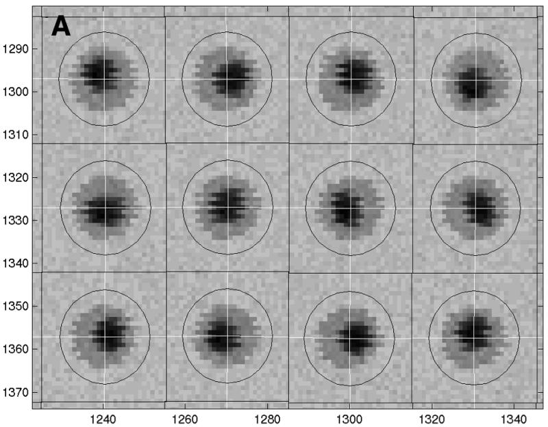
Spot detection and signal acquisition. (A) The image is segmented into spot patches, grids are overlaid to locate spot centers and circular masks are defined to separate the signal region from the background region. (B) Signal acquisition algorithm.

This signal segmentation method utilized both spatial (the spot is inside the circular mask) and intensity (signal should be higher than background noise) information. An integrated algorithm like ours is more accurate than a method purely based on physical location, such as a fixed cell method, and more robust against noise than an edge detection method, which only considers the intensity information. It is a better balance between sensitivity and specificity than either of the methods used alone. Microarray researchers have realized the potential of integrating the two approaches in better classifying signal pixels and in giving more robust and accurate measurement. Many efforts have been made in this direction, notably the Mann–Whitney method (9) and the trimmed measurement method (10). Compared with these methods our method is conceptually simple and intuitive. Moreover, the unique extra iterative procedure we designed can improve spot detection further.

We have tested our program on a set of high density slides from MAC040. This design has 9216 spots on each slide, with the spot-to-spot distance being ∼18 pixels (180 µm) and spot size being ∼12–14 pixels (120–140 µm) in diameter. We found by visual inspection that on average the program is able to locate centers accurately for >99.5% of spots. For those spots for which the program failed to satisfactorily define their centers, the majority (>90%) of them are in problematical regions where even visual determination of spot centers is difficult. Problems include, for example, a very high noise level, close proximity to neighboring spots and extremely irregular spot shapes. Because of the nature of the problematical regions, we believe that data from these areas are much less reliable than from others. Therefore, it is more important to record the problems when querying the quality of data than to try to laboriously and often unsuccessfully align the grids in these regions. We will address this issue in more detail in the following section, when we will define a few parameters to assess the quality of data acquired from each spot.

RESULTS

Spot quality determination

The reliability of the data is affected by multiple factors, ranging from problems in array fabrication and hybridization to image processing. We investigated the following five most common problems encountered in image processing and defined a quality score for each: spot size irregularity, signal-to-noise ratio, local background level and variation and intensity saturation. These five scores were then combined into a composite quality score to reflect the overall quality of the spot being assessed.

Size of the spot. Spots with smaller than usual size combined with high intensity should be penalized, since they are more likely due to isolated noise than dye incorporation due to hybridization; spots with an excessively large diameter, on the other hand, may indicate contaminants in close proximity and/or that the spot is likely to be too close to its neighbors. Either can imply that the printing and/or hybridization conditions are not optimized. We define a quality score for each spot to record size irregularity as

1

where A is the area of the spot, measured by the number of signal pixels, A₀ is the average spot area and ÔxÔ is the absolute value of x. Notice that the normalization condition is automatically satisfied by the above definition.

Signal-to-noise ratio. The signal-to-noise ratio quantifies how well one can resolve a true signal from the noise of the system. Typically the background noise is used for the computation. It is clear that when the signal-to-noise ratio is low, the intrinsic variation in the data is high and confidence in the accuracy of the data is low. Therefore, we define a second quality score for each dye channel of each spot as

q_sig–noise = 1 – [bkg_l/(sig + bkg_l)] = sig/(sig + bkg_l) 2

where sig is the mean intensity level of the spot and bkg_l is its mean local background.

Local background variability. A third quality score is defined for each dye to reflect the variation in local background noise, since it is an indicator of contaminants in the area and to some extent directly affects the accuracy of the data extracted from signal pixels (our algorithm uses background + 2 SD as the signal threshold),

q_bkgl = f₁/CV_bkg 3

where CV_bkg is the coefficient of variation of the local background and f₁ is a normalization constant that satisfies max(q_bkg1) = 1.

Excessively high local background. Problematical regions on a microarray slide often have higher than average background noise and for that reason we define a second quality score for the local background in each dye channel as

q_bkg2 = f₂{1 – [bkg_l/(bkg_l + bkg₀)]} 4

where bkg₀ is the global average of background noise and f₂ is a normalization constant that satisfies max(q_bkg2) = 1.

Saturation in photo intensity detection. Saturation happens when spot pixel intensity values exceed the detection range of the photomultiplier tube or the electron detector. It usually occurs in spots of highly expressed genes or spots that contain contamination, since it typically results in a strong intensity value. The saturation issue poses a different problem compared with the other issues discussed earlier. When irregularities in spot size or shape happen or when noise is high and variable one expects the inherent variability in data measurements to be high and indeed this is true, as we will show in the following section. On the other hand, when saturation happens, there is no prior reason for the variability in measurements to be high. Instead, the measurement distribution is shifted from that when there is no saturation, especially when the instrument settings have not been adjusted to give a ratio of 1 for mRNAs of the same abundance in the two samples (as the quantum yield of the two dyes are different), and both false positives and false negatives are likely. In view of this, instead of constructing a continuous function q_sat, we define a threshold of tolerance of the deviation shift. For spots with a number of saturated pixels above this threshold, we simply discard them. To determine a sensible threshold value, we used synthetic spots of Gaussian shape to assess the effect of saturated pixels on mean or total pixel intensity. The simulation indicates that when the number of saturated pixels is small, error is small. For example, when there is <5% saturated pixels, the error in mean intensity value is <3%; at 10% saturation, the error is still <8%. However, when the number of saturated pixels is >10%, the error increases rapidly. A typical spot on a microarray image has ∼150–250 signal pixels and 10% correspond to ∼20 pixels. We have decided to use 10% as a cut-off value and define a quality score q_sat for each dye to be

5

This score is defined under the assumption that we use the mean or total pixel intensity value. Note that the median value of pixel intensity is less sensitive to variations in the two tails if the intensity distribution is unimodal and would be less affected by the saturation problem. In fact, theoretically, if the number of saturated pixels is <50%, the median pixel intensity is not affected, and we will use 50% as the cut-off value. Since mean intensity is less affected by variations in the pixel intensity distribution, which is determined by the amount of cDNA deposited on each pixel in the spot and is not always unimodal, we will use the mean for our analysis unless otherwise specified and use equation 5 for q_sat.

For the last four quality scores defined for both dye channels a geometric mean will be taken as the corresponding overall quality score for that factor, namely

6

Composite quality score q_com. To give an overall assessment of the spot quality one may design a function to reflect the magnitude of each type of problem, by giving each individual quality score an appropriate weight. For simplicity as well as for the fact that the true weights are unknown, we have for now defined the composite quality score as

q_com = (q_size × q_sig–noise × q_bkg1 × q_bkg2) × q_sat 7a

or

7b

q_sat is treated differently from the other four quality scores because of its dichotomous nature.

Data reliability and spot quality

The above quality scores are constructed to gauge the quality and reliability of the data we acquired from each spot on a microarray image. Therefore, by using the quality score we can assign a measure of confidence to the data. In this section we will investigate the relationship between data reliability and the spot quality scores through the following approaches.

Variation in ratio measurement versus quality scores. According to the experimental design of MAC010 and MAC030 the ratio of Cy5 to Cy3 dye intensities should be uniform across the whole slide, although for slides from MAC030 the intensity values from different spots can be of any value. These slides served as good model systems to investigate data variability versus quality scores. Figure 2 shows scatter plots between (log-transformed) intensity ratios and spot quality scores q_size, q_sig–noise, q_bkg1 and q_bkg2 for a typical MAC030 slide. Evidently, although there are differences in the detailed characteristics of the relationship between ratio and individual quality scores, the general trend is the same, i.e. the ratios derived from spots of high quality scores fall into a much tighter distribution as compared with spots of low quality scores. This suggests that the variability in ratios is due primarily to the variability in spot quality. We did not show a correlation with q_sat because of its dichotomous format and because, as discussed above, we expected saturation to cause deviations of measurement distributions from the true one rather than to contribute significantly to data variability.

Figure 2.

The correlation between variability in intensity ratio measurements and individual quality scores.

Figure 3 shows the variation in intensity ratio values as a function of the composite quality score for the same slide as used in Figure 2. Clearly q_com correlates remarkably well with the variability in ratio measurements. Ratios from spots with high q_com are much less variable than spots with low q_com. The results suggest that q_com can be used as a good measure of variability in ratio measurements.

Figure 3.

The variability in intensity ratio measurements is correlated with q_com.

Consistency of results from replicates and duplicates is correlated with q_com. We had multiple slides from each design and slides from MAC030 had two replicate sets of spots on each. We used these slides to investigate the consistency of results from duplicates/replicates and to see whether more consistent results can be achieved by removing bad spots as judged by their low q_com. Figure 4A plots the ratio of ratio measurements from two duplicate MAC040 slides against the geometric mean of q_com between them. It is clear that for spots of high quality in both duplicates the measurements are very consistent, whilst when spot quality is low in one or both duplicates, the measurements can differ enormously. To quantify this observation further, we calculated Pearson correlation coefficients between log-transformed ratio measurements from the two duplicates using different cut-off values of q_com, and give the results in Figure 4B. Obviously, discarding poor quality spots greatly improves data consistency between the two duplicates. For example, the correlation between the two whole sets of duplicates was very low (<0.1), with almost no difference from two random sets of 9216 data points; however, if we discard spots with q_com < 0.3, the correlation coefficient quickly increases to 0.88, and if we only retain spots with q_com > 0.5 it increases further to 0.94. Similar results have been found for data from replicates on the same slide.

Figure 4.

Consistency of results between two duplicate MAC040 slides and dependence on spot quality. (A) The ratio of the intensity ratio measurements from slide 1 versus that from slide 2 is plotted against the geometric mean of q_com over two duplicates. (B) The Pearson correlation coefficient between the two duplicates is plotted against cut-off values of q_com.

Consistency of results from different image processing programs. We compared Matarray with two commercially available packages, ImaGene (BioDiscovery, Los Angeles, CA) and Array Vision (Imaging Research, Ontario, Canada). We found that in general the three packages give fairly consistent results. For example, Figure 5A gives a scatter plot of ratio measurements using ImaGene versus that using Matarray for a slide from MAC030. Clearly, for a majority of the spots the correlation between the two packages is very good. There are some spots that yield inconsistent results and we envisage that these outliers are mostly spots of poor quality. This is indeed true, as one can see from Figure 5B, where the 10% of spots with the lowest q_com have been removed.

Figure 5.

Intensity ratio measurements obtained using Imagene compared with those obtained using Matarray for the cases when (A) all spots were included and (B) 10% of spots with the lowest q_com were discarded.

Different image processing algorithms should give the same result for an image of good quality. However, when there is significant noise or irregularities in the image, the results can be rather different. To illustrate and quantify this assertion further, we calculated Pearson correlation coefficients between the log-transformed ratio measurements obtained using the three packages, applying different cut-off values for q_com. The results for a MAC030 chip are given in Figure 6. This figure shows that the correlation between different packages can be quite low if we include all spots on the slide. However, when we remove poor quality spots, the correlation dramatically improves. We found that for spots with a quality score >0.85, the correlation coefficients are usually >0.9 among the three packages for all slides tested from the three designs.

Figure 6.

Consistency of results between different microarray image processing packages also depend on spot quality score.

Dependence of data variability on q_com. We have investigated the characteristics of ratio measurements distribution versus q_com in more detail. To do so we used slides from MAC040, for its high density (9216 clones on each) and more realistic experimental design (samples from two different origins were used in each hybridization). We found that distribution of the log-transformed ratio measurements is essentially bell-shaped at all quality levels, with the spread of distribution dependent on q_com. We further quantified this relationship by calculating the variance of the distribution and correlating it with the quality score. For each set of 9216 spots we sort the data according to q_com and divide them into 18 bins each with 500 spots (discarding the lowest 216 spots, which always have q_com < 0.01). Mean q_com and variance σ² of the log(ratio) distribution were calculated for each bin and the results for a typical slide are given in Figure 7A. The relationship between the variance σ² and q_com seems to resemble an exponential decay. This was confirmed in an empirical fitting to the log-transformed variance log(σ² – σ²₀), where σ²₀ is the asymptope of σ² at q_total→1, as shown in Figure 7B. The straight line is the least- square linear fit to the data. It is clear that dependence of log(σ² – σ²₀) on q_com is linear. For the data shown in Figure 7B, the coefficient of determination r² of the linear regression is 98% and P < 0.0001. For all slides (seven) tested in general (six of seven) the r² values were >90%, indicating that the linear model fits the data very well and that indeed the variance in ratio measurement drops off exponentially as q_com increases. One slide where there is no significant correlation between variation and spot quality score does not fit this linear model. Under visual inspection this slide seems to have an excessively high background with several visible stains of regular geometrical shape. These characteristics suggest that non-random factors are affecting the quality of this slide and special care other than the processes we described should be taken.

Figure 7.

Variance σ² of the log-transformed ratio depends on q_com. (A) σ² decreases with increasing q_com. (B) Log-transformed σ² depends linearly on q_com.

Note that log(ratio) = log(Cy5) – log(Cy3) and its variance var[log(ratio)] is related to the variance of individual dyes by

var[log(ratio)] = var[log(Cy5)] + var[log(Cy3)] – 2 covar[log(Cy5), log(Cy3)] 8

In Figure 8A we give the plot of variances var[log(ratio)], var[log(Cy5)] and var[log(Cy3)] and covariance covar[log(Cy5), log(Cy3)] as functions of q_com for the slide shown in Figure 7. From this figure one can see that for the first few data points with q_com < 0.4 the improvement in ratio measurement is mainly due to an improvement in the measurement of individual dyes. However, for spots with q_com > 0.4, the variances in the individual dye intensities do not change much with increasing q_com and the drop in var[log(ratio)] seems to be mainly due to an increase in covar[log(Cy5), log(Cy3)]. These data points correspond to the top 7000 spots (76%) in quality. Remember that the behavior of the correlation coefficient between the two dyes covar[log(Cy5), log(Cy3)]/ is largely determined by the behavior of covar[log(Cy5), log(Cy3)] when both var[log(Cy5)] and var[log(Cy3)] are constants. Therefore, for the majority of spots that are not in the extreme low quality region the improvement in correlation between the two dyes is more significant than the improvement in variability of the individual dye intensities as spot quality improves and the exponential decay of var[log(ratio)] with increasing q_com is largely due to the contribution from the improvement in correlation between the two dyes. We have calculated the Pearson correlation coefficient between the two dyes, transformed it by log(1 – correlation coefficient) and give the plot in Figure 8B. Clearly, except for the first data point, the transformed correlation coefficient essentially depends linearly on q_com, indicating that the correlation between the two individual intensities does indeed improve exponentially with increasing q_com.

Figure 8.

Dependence of var[log(ratio)] on q_com. (A) Variances of ratio and individual intensities and covariance between the two dyes plotted against q_com. (B) The transformed correlation coefficient between the two dyes plotted as a function of q_com. The solid line shows the least squares linear fit to the data.

DISCUSSION

Microarray technology is still in its infancy, and making good chips and getting consistent results are an art. Many factors affect the quality of the final image data: quality of clone preparation, printing, quality of RNA, and hybridization, to name a few. Each and every step in obtaining the final image data can affect the final quality of the image data, causing variations in intensity readings and, in turn, the ratios. Using a composite quality score q_com we have demonstrated in this paper that the variability in intensity ratios used extensively by all microarray investigators is due in large part to the quality of image spots and that q_com acts as a good measure of data variability and can be utilized to gauge and remove inferior spots in order to improve data reliability. In addition, we have found that the variability in intensity ratios decreases exponentially with increasing q_com, further indicating that the variability can indeed be substantially reduced by choosing quality spots. Given the imperfections that are routinely encountered in making cDNA chips, the aforementioned results immediately suggest the necessity of quality evaluation of each and every spot in a microarray slide. Without this quantitative quality check, any sophisticated data analytical method will not yield the intended results.

Our study has also shown that the consistency between duplicate/replicate data sets depends closely on spot quality. Data from high quality spots are highly consistent across replicates/duplicates whilst that from poor quality spots can be totally irrelevant. This result is both important and intuitive and we think it may help to explain a phenomenon of microarray technology that has troubled many scientists. Many reports have shown that the correlation between replicates on the same slide or between duplicate slides is not ideal (11). To overcome this problem, some choose to add different clones rather than replicates if there is extra space on a slide (12); others suggest that adequate numbers of replicates and duplicates should be made to reduce false positives (11,13). We have shown that poor correlations between replicates and duplicates are mostly caused by spots of poor quality and, therefore, it is crucial to be able to tell them apart from spots of good quality before one makes use of replicate and duplicate data and performs complex analyses. Without an objective and quantitative scheme to do so, comparing replicates/duplicates could lead to spurious results.

The definition of spot quality scores is a complex issue; designing parameters that capture the major problems in a microarray image and constructing a composite score that delicately balances the consequences of each individual problem requires a lot of work. It should also be pointed out that there are factors causing variability that cannot be captured by the use of composite quality scores. For example, if an arrayer uses multiple pins that give rise to non-uniform dots, additional variations in intensity ratios can be introduced. Here we do not propose that we have solved the quality control problem, rather, we think it is an issue that needs to be worked out among array users. For example, one may want to use the minimum of all individual quality scores as an overall assessment, namely defining q_com = min({q_i}). We have looked into this case and found that the results are similar to using equation 7. Another possibility is to define q_com = Π q_i^n_i, where n_i are weights of the individual quality scores. Users may want to choose the values each time according to the magnitude of each problem on the image or each laboratory may come up with its own set of optimized {n_i}. One might also find that one needs to use a set of individual parameters corresponding to the common quality problems in microarrays and set a threshold for each, rather than defining a composite quality score. We hope that our work will serve to start an active discussion on this matter. A proper standardized quantitative quality control procedure for microarrays independent of instruments or software packages being used will not only generate reliable data for complex data mining tools, but also truly make the automation of microarray image analysis and data sharing from different laboratories feasible and practical.

Quantitative study of the relationship between data variability and spot quality is also significant because it may reveal to us the intrinsic principles governing the variability in microarray data and may be used to help identify the cause(s) of the imperfection. Furthermore, the results suggest the possibility of a quality metric-dependent filtering and normalization procedure. It is known that there is more variation in measurement when spot intensities are low and the canonical approach many array researchers take is to set threshold values for each dye and only use spots above the threshold for further analyses (14,15). Usually the means and SD of the log-transformed ratios of the retained spots were calculated, those further than a certain number of (for example 3) SD away from the mean are identified and the transcripts deposited at these spots are considered to have exhibited differential expression in the two samples (14,16). Intensity level thresholding is equivalent to filtering using the signal-to-noise ratio (q_sig–noise) when the background noise is uniform. We have found that q_com correlates with the variation in measurement much better than intensity values. As one can see from Figures 2–4, the variability in ratio measurements not only depends on the signal-to-noise ratio but also depends on spot size and local and global variations in background noise. This result suggests that q_com can be a better gauge for data filtering and one may take either of the following two approaches to utilize it. (i) Set a threshold value for q_com. Only spots above this value will be kept and they will be treated with the same statistics as outliers. (ii) Adopt a quality metrics-dependent gauging process. Figure 9 illustrates such a possible new filtering and normalization scheme. In Figure 9 a scatter plot of log(ratio) is given against q_com; solid lines are means of log(ratio) ± 3σ, where σ is the SD calculated using the best fitting line in Figure 7B. Spots outside these two lines can be considered to have significant differential expression between the two samples. Obviously this scheme has the potential for more sensitive detection at the high quality end and for generating far fewer false positives in the low quality region.

Figure 9.

The dependence of variability in ratio measurements on spot quality can be used as a new gauging scheme for outliers.

AVAILABILITY

The Matarray package is available free of charge. Interested users may contact the corresponding author.

References

- 1.Brown P.O. and Botstein,D. (1999) Exploring the new world of the genome with DNA microarrays. Nature Genet., 21 (suppl. 1), 33–37. [DOI] [PubMed] [Google Scholar]
- 2.Debouck C. and Goodfellow,P.N. (1999) DNA microarrays in drug discovery and development. Nature Genet., 21 (suppl. 1), 48–50. [DOI] [PubMed] [Google Scholar]
- 3.Khan J., Bittner,M.L., Chen,Y., Meltzer,P.S. and Trent,J.M. (1999) DNA microarray technology: the anticipated impact on the study of human disease. Biochim. Biophys. Acta, 1423, M17–M28. [DOI] [PubMed] [Google Scholar]
- 4.Diehn M., Alizadeh,A.A. and Brown,P.O. (2000) Examining the living genome in health and disease with DNA microarrays. J. Am. Med. Assoc., 283, 2298–2299. [PubMed] [Google Scholar]
- 5.Eisen M.B., Spellman,P.T., Brown,P.O. and Botstein,D. (1998) Cluster analysis and display of genome-wide expression patterns. Proc. Natl Acad. Sci. USA, 95, 14863–14868. [DOI] [PMC free article] [PubMed] [Google Scholar]
- 6.Tamayo P., Slonim,D., Mesirov,J., Zhu,Q., Kitareewan,S., Dmitrovsky,E., Lander,E.S. and Golub,T.R. (1999) Interpreting patterns of gene expression with self-organizing maps: methods and application to hematopoietic differentiation. Proc. Natl Acad. Sci. USA, 96, 2907–2912. [DOI] [PMC free article] [PubMed] [Google Scholar]
- 7.Zhang M.Q. (1999) Large-scale gene expression data analysis: a new challenge to computational biologists. Genome Res., 9, 681–688. (Erratum, Genome Res., 1999, 9, 1156] [PubMed] [Google Scholar]
- 8.Schena M., Shalon,D., Heller,R., Chai,A., Brown,P.O. and Davis,R.W. (1996) Parallel human genome analysis: microarray-based expression monitoring of 1000 genes. Proc. Natl Acad. Sci. USA, 93, 10614–10619. [DOI] [PMC free article] [PubMed] [Google Scholar]
- 9.Chen Y., Dougherty,E.R. and Bittner,M.L. (1997) Ratio-based decisions and the quantitative analysis of cDNA microarray images. J. Biomed. Optics, 2, 364–374. [DOI] [PubMed] [Google Scholar]
- 10.Zhou Y.-X., Kalocsai,P., Chen,J.-Y. and Shams,S. (2000) Information processing issues and solutions associated with microarray technology. In Schena,M. (ed.), Microarray Biochip Technology. BioTechniques Books, Natick, MA, pp. 167–200.
- 11.Lee M.L., Kuo,F.C., Whitmore,G.A. and Sklar,J. (2000) Importance of replication in microarray gene expression studies: statistical methods and evidence from repetitive cDNA hybridizations. Proc. Natl Acad. Sci. USA, 97, 9834–9839. [DOI] [PMC free article] [PubMed] [Google Scholar]
- 12.Golub T.R., Slonim,D.K., Tamayo,P., Huard,C., Gaasenbeek,M., Mesirov,J.P., Coller,H., Loh,M.L., Downing,J.R., Caligiuri,M.A., Bloomfield,C.D. and Lander,E.S. (1999) Molecular classification of cancer: class discovery and class prediction by gene expression monitoring. Science, 286, 531–537. [DOI] [PubMed] [Google Scholar]
- 13.Manduchi E., Grant,G.R., McKenzie,S.E., Overton,G.C., Surrey,S. and Stoeckert,C.J.,Jr (2000) Generation of patterns from gene expression data by assigning confidence to differentially expressed genes. Bioinformatics, 16, 685–698. [DOI] [PubMed] [Google Scholar]
- 14.DeRisi J., Penland,L., Brown,P.O., Bittner,M.L., Meltzer,P.S., Ray,M., Chen,Y., Su,Y.A. and Trent,J.M. (1996) Use of a cDNA microarray to analyse gene expression patterns in human cancer. Nature Genet., 14, 457–460. [DOI] [PubMed] [Google Scholar]
- 15.Khan J., Simon,R., Bittner,M.L., Chen,Y., Leighton,S.B., Pohida,T., Smith,P.D., Jiang,Y., Gooden,G.C., Trent,J.M. and Meltzer,P.S. (1998) Gene expression profiling of alveolar rhabdomyosarcoma with cDNA microarrays. Cancer Res., 58, 5009–5013. [PubMed] [Google Scholar]
- 16.Tavazoie S., Hughes,J.D., Campbell,M.J., Cho,R.J. and Church,G.M. (1999) Systematic determination of genetic network architecture. Nature Genet., 22, 281–285. [DOI] [PubMed] [Google Scholar]