Mechanics and Dynamics of Actin-Driven Thin Membrane Protrusions

Abstract

Motile cells explore their surrounding milieu by extending thin dynamic protrusions, or filopodia. The growth of filopodia is driven by actin filament bundles that polymerize underneath the cell membrane. We compute the mechanical and dynamical features of the protrusion growth process by explicitly incorporating the flexible plasma membrane. We find that a critical number of filaments are needed to generate net filopodial growth. Without external influences, the filopodium can extend indefinitely up to the buckling length of the F-actin bundle. Dynamical calculations show that the protrusion speed is enhanced by the thermal fluctuations of the membrane; a filament bundle encased in a flexible membrane grows much faster. The protrusion speed depends directly on the number and spatial arrangement of the filaments in the bundle and whether the filaments are tethered to the membrane. Filopodia also attract each other through distortions of the membrane. Spatially close filopodia will merge to form a larger one. Force-velocity relationships mimicking micromanipulation experiments testing our predictions are computed.

INTRODUCTION

In the crawling movement of eukaryotic cells, two types of membrane protrusions, lamellipodia and filopodia, are often observed. A lamellipodium is a flat and broad membrane extension filled with a dense and highly branched actin filament meshwork (1,2). Filopodia are needlelike membrane extensions occupied by aligned actin filaments organized into bundles (3–7). In both types of protrusions, actin filaments are polarized, with their fast-growing barbed ends pointing in the direction of cell motion and their pointed ends pointing toward the cell body. Cells extend filopodia from the lamellipodium (8) to explore their surrounding milieu. A nascent filopodium forms when the actin-bundling protein Fascin fuses individual actin filaments into ordered bundles (5). The elongation of the filopodium can progress for several microns. Force generation through actin polymerization has been studied extensively (9,10), but how the presence of the plasma membrane affects force generation and membrane protrusion dynamics is not well understood. In this article, we quantify the process of actin-powered filopodium extension using a computational model. We couple explicitly actin polymerization kinetics with the fluctuation dynamics of the plasma membrane to compute the protrusion speed as a function of the number of filaments in the bundle and the cell membrane elasticity, although the process of filopodia initiation is not explicitly modeled.

Electron microscopy of growing filopodia at the leading edge of mouse melanoma cells suggests that cross-linked F-actin bundles make up the filopodium (11,12). The number of actin filaments and the density of cross-linking proteins (Fascin) determine the rigidity of the bundle (13–15). The base of the filopodium is anchored in the highly cross-linked F-actin network of the lamellipodium (11,16,17). Under physiological conditions, most filopodia extend at a speed of ≈0.2 μm/s, growing up to 2-μm in length (11,18,19). After a critical length is reached, the filaments appear to buckle and the filopodium dissolves (5). Several auxiliary proteins are also found at the tip of the filopodia and may be implicated in the protrusion process (20,21). Models of filopodium growth have been limited to the classical Brownian ratchet model where the filopodium is described as a rigid diffusing object pushed by a single growing filament (10). The effects of actin bundles and the presence of the cell membrane have not been examined previously.

Static energetic considerations alone suggest that the presence of the membrane changes fundamentally the behavior of protruding F-actin bundles. We find that the restoring force exercised by the membrane pointing in the direction opposite to the protrusion direction is roughly constant. A single filament is not sufficient to overcome this restoring force; ∼2–3 growing actin filaments are necessary to produce significant extensions. Due to the membrane restoring force, the actin bundle undergoes a buckling instability when the filopodium reaches a critical length. An F-actin bundle of sufficient stiffness is required to extend the plasma membrane beyond several hundred nanometers. Therefore, even though a small number of filaments already have more than enough chemical polymerization energy to protrude, only a bundle with many filaments is stiff enough to protrude for microns. Membrane mechanics also defines the geometrical features of the filopodium: for instance, the membrane encasing the F-actin bundle has a well-defined radius related to the membrane elastic constants.

When the dynamical properties of the membrane are taken into account, we find that the protrusion speed depends on the elastic properties of the cell membrane. In contrast with the classic Brownian ratchet model, here, the membrane at the tip of the filopodium is flexible. We examine the protrusion dynamics in the limits of a rigid and flexible membrane tip. We also examine two mechanisms of force generation: 1), the Brownian ratchet model (10,22), where the fluctuations of the cell membrane leave sufficient space for the addition of actin monomers; and 2), the tethered ratchet model (23), where the F-actin filaments are physically attached to the cell membrane.

Other theoretical and computational studies have attempted to quantify cell motility (22,24–26). Mogilner and Rubinstein (27) specifically examined the physical parameters during filopodial protrusion. They also computed the F-actin bundle rigidity and the diffusion process of the actin monomers. Others have examined the kinetics of multifilament bundle growth (28–30). Here, we explicitly incorporate the dynamical properties of the cell membrane. Indeed, the most important lesson of this work is that cell protrusion dynamics depends sensitively on the physical properties of the plasma membrane. The membrane has an important influence on the geometry of the actin network and the cell dynamical properties, such as the protrusion growth speed.

STATIC ENERGETIC CONSIDERATIONS

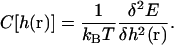
In this section, the static energetics of the filopodium protrusion process is examined using a coarse-grained theory. The mechanical energy of the membrane can be written in the Canham-Helfrich form (31,32) of

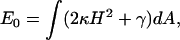(1)

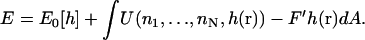
where H is the mean curvature of the membrane and dA is an area element. The values κ and γ are the bending modulus and the surface tension of the membrane, respectively. Contributions due to Gaussian curvature can be considered as boundary energy (33). If we consider a cylindrical symmetry, a point on the membrane can be characterized by two variables, (r, h(r)). Using the Monge representation, the mean curvature is given by

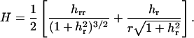(2)

An area element is 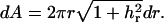Under a fixed protrusion length l, we impose the boundary conditions of h(0) = l and h(∞) = 0, mimicking the effect of membrane adhesion to other parts of the cytoskeleton. The equilibrium membrane geometry can be solved by minimizing the Helfrich energy. The resulting Euler-Lagrange equations are too cumbersome for convenient computation. Instead, we write h(r) as an expansion over a basis set and directly minimize the Helfrich energy with respect to the expansion coefficients. A typical membrane profile is displayed in Fig. 1 a.

FIGURE 1.

Equilibrium membrane energy as a function of the length of the protrusion, l, obtained from minimization of the Helfrich energy. (a) The membrane profile, h(r), is written as a series expansion and then expansion coefficients a_n varied until the minimum energy is reached. The value r′ = 500 nm is the radius of the outer boundary and h(0) = l, h(r′) = 0. For the particular profile shown, l = 1000 nm. (b) For relatively long protrusions, E is a linear function of l. The slope is given by 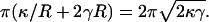For shorter protrusions, the energy profile is nonlinear. The inset shows the energy of the membrane for protrusions up to 50 nm.

The membrane energy as a function of the protrusion length displays two regimes (Fig. 1). For short protrusions, the membrane resembles a smooth bump and the overall mechanical energy grows quadratically with l. As l increases beyond 80 nm, the membrane forms a cylinder of a well-defined radius. An increase in l simply elongates the cylinder length. For long protrusions, the energy of a membrane cylinder is approximately given by

(3)

where R is the cylinder radius. The membrane energy is linear in l. Minimizing with respect to the radius gives Thus, the resorting force in the z direction is given by

(4)

Similar estimates have been obtained for membrane tethers (34).

We asked whether a single actin filament is sufficient to extend a filopodium. Energetic considerations suggest that the answer depends on the bending modulus, κ, and the surface tension, γ, of the membrane. If the free actin monomer concentration in the cell is (actin) = 10 μM, the free energy of a growing actin filament decreases −k_BT ln((actin)/(actin)_c) = −4.4 k_BT per monomer. The critical actin concentration (for the barbed end) is (actin)_c = 0.12 μM. Each added monomer increases the filament length by ∼Δ = 2.8 nm. Thus, the free energy decreases as 1.6 × l, per actin filament. On the other hand, the energy of the membrane, when a cylindrical protrusion has formed, grows as E₀ = −fl where f is given in Eq. 4. For typical plasma membranes, κ ≈ 20 k_BT (35,36) and γ ≈ 0.005 k_BT/nm² (36). This gives f = −2.8 k_BT/nm. Thus, from energy balance alone, a single filament is unable to protrude at all. At least two filaments are needed to overcome the membrane restoring force. For a single actin filament to protrude indefinitely, the free actin concentration has to be at least 500 μM.

We note that the actin filament bundle must be anchored to the cytoskeleton to provide any protrusive force. Here, we assume that the underlying cytoskeletal network is rigid. Additionally, because the pointed end is embedded in the actin filament meshwork, we assume that no depolymerization can occur.

If the flexibility of the actin filaments is taken into account, then buckling and breaking would occur after a critical growth length is reached. The restoring force of the membrane, f, acts as an external force on the semiflexible actin filament. Ignoring thermal fluctuations, there is a critical force, f_b, for which if f > f_b, the filament begins to buckle. A standard calculation (37) gives

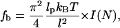(5)

where l_p is the persistence length of the filament and l is the overall length of the filament. For a single actin filament, l_p = 17 μm (38), and I(N) is a dimensionless factor representing the bundle stiffness as a function of the number of filaments in the bundle (27). For the membrane force given by Eq. 4, a single growing actin filament will begin to buckle at l = 170 nm. This result indicates that even though there might be enough chemical energy to drive the growth of a filopodium, a few actin filaments are not stiff enough to extend a filopodium significantly.

The strategy employed by cells to generate thin membrane protrusions is to use F-actin bundles. The persistence length of a filament bundle grows approximately as the number of filaments in the bundle squared, if there are strong cross links between the filaments: i.e., I(N) = N². Therefore, the buckling length grows as the number of filaments. For example, for a bundle of 10 filaments, a filopodium can grow to 1700 nm before the onset of buckling. At forces >f_b, the relative deflection of the filopodium, z/L, is proportional to (37).

Fig. 1 shows that the membrane energy of the filopodium grows linearly as a function of its length. The effective force on the membrane tip is given by Eq. 4. Therefore, a possible model to describe the filopodial protrusion process is to consider an object under the load force given in Eq. 4, and pushed by an F-actin bundle. Dynamical models of filopodium protrusion are discussed in the next section.

Filopodia attract each other

The presence of the plasma membrane introduces an effective attractive force between two filopodia. The length scale of the attraction, d₀, may determine the spacing between filopodia at the leading edge. If the separation between filopodia is within the interaction range, then they will merge to form a larger filopodium. This effect has implications in filopodium formation.

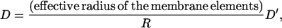
Let the distance between two equal-length filopodia be d (Fig. 2). The unfavorable membrane-energy is minimized if d is zero. From small deformation approximations of the Helfrich theory, the decay length of membrane distortions is ∼ Thus, the interaction distance is d₀ ≈ 4R where R is the radius of a filopodium. Thus, we find that bundles spaced greater than a few hundred nanometers do not interact. The attractive force between the filopodia must also overcome the bending rigidity of the F-actin bundle to merge. Thus, substantial forces may be needed. Therefore, if d > d₀, the filopodia will not merge. With decreasing distance, the membrane between the filopodia will merge and rise toward the tip (Fig. 2, inset). In this regime, the attractive force is quite substantial and depends on the length of the filopodia. To estimate the attractive force, we assume that the lengths and radii of filopodia do not change before and after merging. The change in the membrane energy is ∼2E₀ − E₀ = E₀, where E₀ is the energy of a single membrane tube in Eq. 3. Thus, the effective force, F_a, between filopodia is approximately E₀/d₀, which depends on the membrane properties κ and γ, as well as the length of the filopodia.

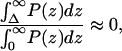
FIGURE 2.

The interaction energy between two filopodia as a function of their separation, d. The energy is minimized when the filopodia merge. The interaction range, d₀, is approximately twice the diameter of the filopodium; d₀ is ≈200 nm. The circles are our computational results and the solid line is a guide to the eye. The dashed line shows the estimated energy using the force estimate of Eq. 6.

Using Eq. 3, we find that the effective attraction force is approximately

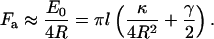(6)

The force is a linear function of l. If l = 500 nm, the force is ∼30 pN.

The relation d₀ ≈ 4R and a more accurate estimate of the interaction energy between filopodia can be obtained by carrying out finite element calculations of the membrane geometry. The computational procedure is given in Appendix A. To find the range of interaction between filopodia, we compute the average membrane energy as a function of d,

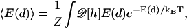(7)

where E(d) is the shape energy of the filopodia, which is given by Eq. A1. The functional integral, represents an integration over all possible membrane configurations, and Z is the partition function. This energy is a measure of the enthalpy of attractive interaction and includes thermal fluctuations. Fig. 2 shows 〈E(d)〉 as a function d for two F-actin bundles of l = 1000 nm. (〈E(d)〉 is a linear function of l; this is not shown in Fig. 2.) In this calculation, F-actin bundles are assumed to be rigid. During the merging process, curved bundles may change the membrane geometry between the filopodia. We have not computed the energy for this situation.

We have shown that F-actin bundles closer than d₀ should merge and form a larger bundle if the bundle lengths are long enough. We speculate that this mechanism could be responsible for the experimentally observed λ-patterns at the base of the filopodium inside the lamellipodium actin network and filopodium initiation (11). The details of the merging event depend on the interaction of the membrane with F-actin and the elastic deformations of the actin bundles. These issues are beyond the scope of this work.

DYNAMICAL MODELS OF FILOPODIUM PROTRUSION

Force generation due to bending fluctuations of growing filaments has been studied extensively (24,26). In these models, the fluctuations of the F-actin tip create sufficient space for the addition of actin monomers. The subsequent relaxation of the bent filaments propels the object (plasma membrane, bacterial cell wall, etc.) forward. These mechanisms depend on the geometry of the actin filament behind the moving object, i.e., the angle of the actin filaments with respect to the object. However, the filaments in the filopodium are parallel to each other and presumably perpendicular to the cell membrane at the leading edge. Bundling proteins, such as Fascin, cross-link filaments tightly together (11). Growth due to fluctuating filaments is an unlikely mechanism for filopodial growth for two reasons:

1. F-actin bundles fused by Fascin are quite rigid; the persistence length of the bundle is tens to hundreds of microns.

2. Being perpendicular to the cell membrane, it is difficult for a fluctuating bundle tip to generate sufficient space for monomer addition.

These reasons have been discussed before by Mogilner and Rubinstein (27). Hence, we assume that for filopodia, the protrusion is mostly due to the thermal fluctuations of the membrane; lateral fluctuations of the F-actin bundle itself will not be considered.

The polymerization ratchet model, where a single polymerizing filament propels a diffusing rigid object, has been studied (10). Here, we consider an N-filament polymerization ratchet model and apply it to filopodial growth. We consider two main models of filament bundle growth:

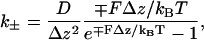
• Model 1. We assume that the tip of the filopodium behaves as a rigid object (cap). The rigid cap can diffuse in the z-direction with a diffusion constant D. In the previous section, we showed that the cell membrane exerts a constant opposing force on the F-actin bundle. Thus, a filopodium may be effectively modeled as a rigid cap under the load force given by Eq. 4 and propelled by the growing bundle (Fig. 3). In this model, the relative stagger of the filaments in the z-direction is important, although the arrangement of the filaments in the x,y-plane is unimportant. Aside from the geometrical arrangement of the filaments, and the bundled morphology of F-actin, this is the classical Brownian ratchet model (10). This model is also similar to the growth of protofilaments in microtubules, for which the force generation properties have been considered before (28,30).

• Model 2. We simulate the flexible cell membrane explicitly and the growth of filopodium is investigated quantitatively (Fig. 3). The dynamics of fluctuating cell membrane is included. The membrane can fluctuate with a diffusion constant D′. (The relationship between D and D′ is discussed in the next section.) Various possible interactions between the F-actin tip and the cell membrane are considered. The detailed formulation of the equations is given in Appendix B. In this model, the arrangement of the filaments in the x,y-plane is important.

FIGURE 3.

Two possible models for describing filopodium extension. The first model (left) is the standard Brownian ratchet model where a F-actin bundle protrudes against a rigid object under load. The rigid object is the tip of the membrane extension, or cap. The load force on the cap is give by Eq. 4. For this model, the spatial arrangement of the bundle in the x,y-plane is of no importance. However, how the filaments are staggered in the z-direction is important. In the second model (right), a flexible membrane is considered. For the flexible membrane, we find that the geometrical arrangement of the filaments is important. In our computation, we vary the spacing between the filaments, d. The physiological spacing is ∼d = 15 nm. In these models, D is the diffusion constant of the rigid membrane cap and D′ is the diffusion constant of the small membrane elements.

Our aim is to compare the two models and demonstrate the effect of the cell membrane. The mathematical details of the models are given in Appendices B and C.

Force generation from a growing bundle of F-actin is significantly different from the single-filament situation (28–30). The protrusion dynamics depends on the spatial arrangement of the filaments in the bundle. The growth of the filaments is stochastic: the lengths of the filaments at any given moment are likely to be unequal. As a result, the object being pushed does not have to diffuse the full 2.8-nm distance to add another monomer. The protrusion speed is significantly higher if there are many filaments in the bundle. This is explored in more detail in Results.

RESULTS

The diffusion constant of an object being propelled depends on the viscosity of the surroundings and the shape of the diffusing object. Under normal cellular conditions, cytoplasmic viscosity can range from 0.03 poise (39,40) to 30 poise (39,41,42); the size of the objects (molecules) may vary from nanometers to microns. Therefore, the diffusion constant can range from 1 to 10⁷ nm²/s. For the sake of generality, we compute the protrusion dynamics for a wide range of D. Note that D for Model 1 is related to D′ of Model 2. D describes the transverse diffusion of the complete membrane cap and D′ describes the transverse diffusion of a small membrane element. Since the diffusion constant of a platelike object in the transverse direction is related to its horizontal dimension, then the relationship between D and D′ is

(8)

where R is the radius of the membrane cap. Results from Model 1 will be compared with those of Model 2 by scaling the diffusion constant with Eq. 8.

In Model 2, the fluctuations of the membrane are potentially coupled via hydrodynamic interactions. In Appendix C, we argue that this coupling is negligible when considering filopodium growth.

We also investigate the speed of filopodial growth as a function of the number of filaments in the bundle (N). We assume that the free actin monomer concentration, (actin), is the same as that of the cytosol. This approximation is valid for filopodia shorter than several microns (27). Throughout the article, (actin) = 10 μM (43). The details of the model parameters can be found in Appendix C. Note that no fitting of parameters was needed: all parameters are either taken from the literature or estimated.

Model 1: bundled filaments propelling a rigid cap

Fig. 4 a shows the protrusion speed as a function of the diffusion constant for a F-actin bundle propelling a rigid membrane cap (Model 1). In the rapid diffusion limit where D/Δ² is much larger than the monomer addition rate, all protrusion speeds approach a plateau value, although the plateau value depends on N. Fig. 4 b shows the dependence of speed on N. In the rapid diffusion limit, the protrusion speed approaches an asymptotic curve.

FIGURE 4.

Model 1: a rigid cap being propelled by an F-actin bundle. The external force, F, is 13 pN, given by Eq. 4. (a) Velocity as a function of the log of the diffusion constant, D, for various number of filaments. (b) The protrusion speed as a function of number of filaments, N, for different values of D.

When D is high, the protrusion velocity is a function of the polymerization kinetics of F-actin and the number of filaments, N. An estimate of the protrusion velocity in this limit can be obtained by assuming that the cap is in thermal equilibrium with respect to z-diffusion. In this limit, the position of the cap satisfies the equilibrium distribution, To examine the effect of filament geometrical arrangement, we first consider two filaments staggered by Δ/2 (Fig. 5). The protrusion velocity in this case is approximately

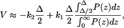(9)

where we have assumed that

(10)

and neglected pathways where two or more successive additions to the same filament occur. This assumption is valid when FΔ ≫ k_BT. For the filopodium, FΔ = 8 k_BT and therefore the assumption is valid. Note that this estimate is valid when the filaments are staggered by Δ/2 with respect to each other. For other geometries, the velocities will be significantly different (see the graph in Fig. 5). In general, for N-filaments, velocity is a sensitive function of the relative stagger of the filaments.

FIGURE 5.

For two filaments propelling a rigid object under load, an estimate of the protrusion speed can be obtained in the limit of D → ∞. The steady-state probability distribution can be separated into several regions, each with a protrusion velocity. The total average velocity is a statistical sum of these contributions. The protrusion velocity for two filaments as a function of the stagger spacing, x, is shown on the right. The actin concentration in this case is 100 μM. A load force of 13 pN is applied in the −z direction.

The speed enhancement due to the F-actin bundle mostly arises from the smaller interval, which the object has to diffuse to add a monomer to a filament tip. For N-filaments equally staggered by Δ/N, instead of diffusing a distance of Δ to add a monomer, Δ/N is sufficiently far to ratchet the cap forward. The probability of generating the distance Δ/N is an exponential function of the external force. If the membrane cap is flexible, the same arguments apply. However, in the following section, we will see that the possibility of generating a gap between the membrane and the filaments is tremendously enhanced by membrane flexibility.

Model 2: flexible membrane enhances protrusion speed

We carried out the full dynamical calculation where the cell membrane is allowed to fluctuate. In Fig. 6 a, the protrusion velocities from Models 1 and 2 are compared. When the membrane is flexible, the filopodium protrudes substantially faster. The explanation of this result is the following: when the membrane is flexible, a local fluctuation that generates a gap between the membrane and the filaments is more likely than when the membrane is rigid. The rigid membrane must overcome the full load force, F. A flexible membrane only has to overcome the unfavorable local bending energy, which is substantially lower than FΔ. Once the monomer is added, the membrane prefers to relax to a flat configuration, and the generation of additional space between the membrane and F-actin becomes favorable. Thus, the filaments in fact help each other to grow, via thermal fluctuations of the plasma membrane.

FIGURE 6.

Model 2: comparison between the flexible and rigid membrane, and the effect of the filament arrangement. (a) Protrusion velocity as a function of the diffusion constant for Models 1 and 2. There are 25 filaments in the bundle. The diffusion constants D and D′ are adjusted according to Eq. 8. The inset shows the dependence of the protrusion velocity on the membrane bending constant, κ. The physiological value is κ = 20 k_BT. (b) The effect of the filament arrangement in the bundle: Protrusion velocity drops substantially when the filaments are together (d = 0). Comparison with the rigid membrane is also shown. This result implies that for the flexible membrane, the arrangement of the filaments can have important effects on the speed. The filaments help each other to protrude via the flexible membrane. The diffusion constants D and D′ are again adjusted according to Eq. 8.

To validate this explanation, we carried out the computation for the hypothetical situation where all of the filaments are located at x = y = 0. Thus, instead of the physiological spacing of d = 15 nm, we choose d = 0 nm (Fig. 3 b). The membrane is still flexible; the only difference is the arrangement of the filaments. In Fig. 6 b, the filopodium protrusion speed as a function of the number of filaments in the bundle is compared for these situations. We see that a spatial separation between filaments, which corresponds to the bundle structure, enhances the protrusion velocity.

The protrusion speed can vary, depending on the number of filaments in the bundle. In an experiment where N is known, the effect of membrane flexibility can be observed using our model estimates. The membrane rigidity can be manipulated by depleting or adding cholesterol to the plasma membrane. Our model predicts that the protrusion velocity will change as a function of the membrane rigidity. The inset in Fig. 6 a shows the protrusion velocity as a function of the membrane bending constant, κ. Membrane surface tension or stretch modulus, γ, is held constant.

Force velocity relations

To find the general force-dependence of the protrusion velocity, we compute the protrusion velocity of the bundle under an arbitrary applied force. In Model 1, the load force can be applied directly to the rigid membrane cap. Alternatively, to mimic a possible experiment, the load force can be applied to a rigid bead that obstructs the filopodium growth. We examine both situations using computational modeling.

Fig. 7 a shows the protrusion velocity of the filopodium as a function of the load force, F, in Model 1. Note that the membrane already exerts an opposing force of F = 13 pN if κ = 20 k_BT and γ = 0.005 k_BT/nm². Thus, for filopodia, velocities for forces <13 pN would not be observed. For a small number of filaments (N < 50), the force-velocity relationship shows the standard exponential character. However, for a larger number of filaments, the bundle growth responds to force differently, especially for forces in the physiologically relevant range of 10–20 pN. Force-velocity relationships of this type can be measured for F-actin bundles in reconstituted systems growing against a rigid object (44).

FIGURE 7.

Force-velocity diagrams. (a) Model 1 with a rigid membrane cap. We vary the load force on the membrane cap, F. The dotted lines are the results for rapid diffusion, D = 10⁴ nm²/s. The solid lines are results for slow diffusion, D = 50 nm²/s. The load force arising from membrane elastic energy is between 10 and 20 pN. The dot-dashed line is the elongation velocity of a single actin filament. (b) Force velocity curve in a possible experiment. The comparison between Models 1 and 2 is shown for N = 25. The load force is applied via a large bead at the tip of the filopodium. The diffusion constant for the bead is varied from D₂ = 100 nm²/s to D₂ = 1000 nm²/s. The load force, F′, such as from a laser trap, is applied to the bead. A rigid membrane with D = 2000 nm²/s is compared with a flexible membrane with D′ = 10⁴ nm²/s. Notice that for F′ = 0, the flexible membrane situation is slower than the rigid membrane when D₂ = 100 nm²/s. This is the opposite of the result when D₂ = 1000 nm²/s. This is due to the presence of the slow rigid object, which hinders the protrusion, even for F′ = 0.

To compute the force-velocity relationship of a filopodium in vivo, the load force can be applied using a bead bound by a laser trap, the bead obstructs the growing filopodium. In addition to the fluctuating membrane, the fluctuations of the bead also play a role. Fig. 7 b shows the force-versus-velocity relationships for this situation. The bead has its own diffusion constant, D₂. The bead and the tip of the filopodium are assumed to interact via hard-core potentials. The force-velocity relationship indicates that a rigid membrane produces faster growth velocities when D₂ is small, opposite of the trend in Fig. 6. Interestingly, the obstruction of the bead introduces an unexpected effect. Now, to add monomers, a collective fluctuation of the bead and the membrane is needed. Since the bead fluctuates much more slowly than the flexible membrane, the bead suppresses the small membrane fluctuations that enhance the filopodium growth velocity.

DISCUSSION

Filopodial extension is now recognized as the result of a F-actin bundle, anchored in the lamellipodium network, protruding against the resistive restoring force of the membrane (5,7,10,27). The main purpose of this article is to explore the effects of the plasma membrane on the protrusion of actin bundles, or filopodia. We quantified the mechanical resistance force generated by the membrane, opposing the filopodial growth. We showed that the elasticity of the membrane can generate attractive forces between spatially separated filopodia, potentially bending the F-actin bundles and creating additional reorganization of the leading edge. Dynamical features such as membrane ruffles may be the result of membrane elasticity as well.

The elasticity of the cell membrane also influences the protrusion dynamics of the filopodium. We find that the fluctuations of a flexible membrane can enhance the filopodial growth velocity (see Fig. 8). Several factors/parameters such as the spatial arrangement of the filaments in the bundle, the membrane-bending modulus and diffusivity, and the actin monomer concentration at the tip of the filopodium, are all important in determining the protrusion velocity. Some of these parameters, such as the membrane elastic constants, are known. The transverse membrane diffusion constant, D′, can be measured by analyzing the fluctuating dynamics of stained membrane. Actin monomer concentration at the filopodium tip is more problematic. A possible approach is to compute the actin monomer concentration profile using a reaction diffusion equation (27). However, the actin monomers are not free to diffuse within the filopodium; the presence of the bundle must be incorporated to properly estimate the actin monomer concentration. When the number of filaments in the bundle is large, and the filopodium is long, the growth of the filopodium becomes diffusion-limited (27).

FIGURE 8.

Filaments mutually enhances the growth of the filopodium. Membrane fluctuations are rectified by a growing filament. The subsequent relaxation of the membrane creates more space for the growth of other filaments. The enhancement is a direct function of the membrane flexibility. The same mechanism must also exist for the lamellipodium growth where branched filaments are coupled via membrane fluctuations.

In an in vitro experiment with lipid vesicles, factors influencing filopodium protrusion dynamics maybe controlled. The elastic properties of the lipid vesicle, the amount of cross-linking proteins, and the number of actin monomers can be varied. Quantitative comparison between theory and experiment is then possible.

Membrane fluctuations may play a similar role during lamellipodium protrusion (45). The actin filaments within the lamellipodium are usually not in a bundled form, but branched and cross-linked (46). The protruding filaments at the lamellipodium leading edge should assist each other in the same manner as the filopodium. Depending on the Arp2/3 and the capping protein concentrations, the spacing between the filament tips in the lamellipodium is substantially larger. Thus, the enhancement of the protrusion velocity by the fluctuating membrane may be quantitatively different. Physical attachment (tethering) of the filaments to the leading-edge membrane can also change membrane fluctuation characteristics. The dynamical role of the membrane in the lamellipodium is in need of quantification.

Several proteins, such as Ena/VASP, have been observed to aggregate at the tip of filopodia (20,21). They may mediate the generation of protrusions, very much like other capping proteins that are attached to the membrane (e.g., formin). Force-generation with tethered growing filaments has been studied before (47,48). It is possible that capping of F-actin modifies the polymerization rate constants, k₁ and k₂. In addition, tethering between F-actin and the membrane changes the fluctuation behavior of the leading-edge membrane. The most significant effect of tethering is that it changes the mean time where a sufficient gap is generated between the filament and the membrane. An estimate can be obtained by examining the mean first-passage time of generating a gap of Δ = 2.8 nm. In general, if the tethering protein is a passive mechanical element, then tethering increases the time needed to generate a gap; however, the tethering protein may take advantage of the hydrolysis cycle of actin to actively generate a gap.

This model does not account for the dynamics after the buckling length of the filopodium is reached. When the bundle starts to bend, the increased strain in the filaments will change the polymerization and depolymerization kinetics, and may lead to the breakage of the filaments. In all of these processes, the cell membrane plays a substantial role and, as shown here, must be considered in quantitative models of cell motility.

APPENDIX A: MEMBRANE STATISTICAL MECHANICS WITH FINITE ELEMENTS

During cell movement, filopodia typically extend from the lamellipodium whose thickness is ∼200 nm (46). To incorporate the appropriate boundary conditions and include the thermal fluctuations and statistical mechanics in our computational model, we carried out equilibrium Monte Carlo simulations of filopodia extension from the lamellipodial edge. Fig. 9 shows a snapshot from the simulation. We vary the length of the filopodium by fixing the overall length of the F-actin bundle to be l. The energetics of the system is explored as a function of l. Note that, in this situation, there is no overall symmetry and the membrane must be specified by a three-dimensional coordinate system. To compute the membrane energy, we implemented a finite element representation of the membrane that allows for arbitrary boundary conditions. The membrane is free to fluctuate and change the vertex of the finite elements. The actin filaments in the bundle (not shown in the figure for clarity) are treated as parallel rigid cylinders (6-nm in diameter). The spacing between the filaments from center to center is d = 15 nm. At the tip of the filopodium, the membrane is not allowed to sample configurations below z = l.

FIGURE 9.

Representative membrane configuration obtained from a Monte Carlo simulation. The membrane area is composed of triangular finite elements. (Inset) The membrane energy of a growing filopodium as a function of its length.

To compute the average membrane enthalpy of Eq. 7, the membrane surface, h, is tiled by a triangular lattice of finite elements. Each triangle, indexed by i and characterized by a vector normal to the triangle, a_i, can change its size and orientation. Eq. 1 can be written in a discretized form (49–51),

(A1)

where the i-summation is over all the triangles in the membrane. For each triangle, the j-summation is over all the neighboring triangles of i. l_ij is the length of the edge shared by i and j triangles. Δ_i is the area of the i^th triangle. The values κ and γ are the bending modulus and surface tension of the membrane, respectively. The membrane geometries can be varied by changing the positions of the vertices. By moving the vertices, all possible membrane geometries can be sampled. The functional integral in Eq. 7, symbolizes integration over all possible membrane configurations. The enthalpy average is obtained using the Metropolis Monte Carlo procedure (52).

APPENDIX B: MODEL 1—RIGID CAP PROPELLED BY THE F-ACTIN BUNDLE

We model the tip of the filopodia as a rigid circular disk with the radius and one-dimensional diffusion constant D. A load force, F, is applied in the direction opposite to the protrusion (−z direction). The load force is given by Eq. 4. We treat the F-actin bundle as N-parallel rigid filaments polymerizing (depolymerizing) in Δ = 2.8-nm increments. Note that Δ is one-half of the actin monomer size. The cap can only move in the z-direction and no rotation or change of orientation is allowed (Fig. 3). Therefore, the x,y-positions of the filaments and the relative distances in between the filaments are unimportant. However, the relative positions of the filaments in the z-direction are important. We have assumed that the filaments are evenly staggered by Δ/N in the z-direction.

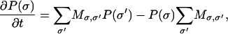
To compute the dynamics, we consider the joint probability, P(z,n₁,…,n_N,t), where N is the total number of filaments and n_α is the number of monomers in the α^th filament. The probability satisfies the equation

(B1)

where k₁ and k₂ are the polymerization and depolymerization rates of F-actin, respectively, and D is the transverse diffusion constant of the rigid cap. F is the load force on the cap. The value of F is given by Eq. 4.

The polymerization kinetics of F-actin has been measured. In our model, we use k₁ = 11.6 (actin) s⁻¹, k₂ = 1.4 s⁻¹ (53).

The probability of adding actin monomers depends on the cap position, z, and the number of monomers in the α^th filament, n_α. This relationship is captured by the function H(z, n_α). If there is sufficient space between the filament and the cap, i.e., z > n_αΔ, then H = 1; otherwise, H = 0.

The solution of Eq. B1 is obtained using a Monte Carlo algorithm. The details of the method are given in Appendix D. The possible kinetic events defining the dynamics are

1. Addition of a monomer with rate k₁ to any of the filaments if the space between the filament and the cap is >Δ.

2. Loss of a monomer with rate k₂ from any of the filaments.

3. Diffusion of the cap against a constant force, F, applied in −z-direction, with a rate k₊ by the amount Δz.

4. Diffusion of the cap with rate k₋ by −Δz, if the cap does not overlap the physical space occupied by the filaments.

The values k₊ and k₋, which must satisfy the detailed balance condition, are given in Appendix D. These rates are valid in the range of small Δz, such that the diffusing cap can be considered to be in a local steady state.

APPENDIX C: MODEL 2—FLUCTUATING FLEXIBLE MEMBRANE PROPELLED BY F-ACTIN BUNDLE

In Model 2, we simulate the membrane and the F-actin bundle interactions by incorporating the flexibility of the membrane. Unlike Model 1, the membrane can adopt any shape. We incorporate realistic interactions between the F-actin tip and the membrane. Unlike Model 1 where the membrane cap is rigid, no external forces are needed since the tension and resistance of the membrane are automatically incorporated. The F-actin bundle in the filopodium has the same properties as defined in Model 1. However, in this model, the geometrical arrangement of the filaments is important. The relative distance between the filaments, d, is taken to be 15 nm to mimic the physiological situation (see Fig. 3). As explained in the text, the arrangement of the filaments in the bundle has important effects on the propulsion dynamics of the filopodium. For the unphysical situation where d = 0 nm, the protrusion velocity is changed substantially. These aspects are discussed in more detail in Results.

To couple the growth of the F-actin with the dynamical movement of the membrane, we examine the forces acting on the cell membrane at the leading edge. In the regime of low Reynolds number, viscous frictional force is balanced by the forces between the membrane and F-actin, and the Brownian random force; we have

(C1)

where r = (x, y) and E(h) is the membrane energy as a function of the membrane configuration and force due to the growing actin bundle. The Oseen tensor, D′(r – r′), describes the viscous friction from the surrounding solvent and hydrodynamic coupling between different membrane locations, and ζ(r, t) is the random force that satisfies the fluctuation dissipation theorem (54). The presence of the actin bundle is contained in the membrane energy E(h) and, therefore, the membrane fluctuations are coupled to the growth of the actin filament bundle. In this article, we make the approximation

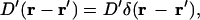(C2)

which simplifies the model enormously. In general, hydrodynamic effects act over large length-scales and cannot be neglected for fluctuating membranes. In this case, however, the filopodium is <100 nm in radius. In this length regime, the internal viscous friction of the plasma membrane is actually more important than hydrodynamics (55). Furthermore, the filopodium grows near the substrate where the velocity field of the fluid is typically damped out by wall effects. With this combination of factors, the approximation of Eq. C2 is justified. However, D′ is now a phenomenological parameter and must be measured for the membrane at the leading edge of crawling cells. In Results, above, we show that D′ is a crucial parameter, which controls the protrusion speed.

To model the joint actin/membrane dynamics, a Fokker-Planck equation can be used to describe membrane movements in the three-dimensional Cartesian space (x, y, h(x, y)) coupled to the filaments (n₁,…,n_N). The time-evolution of the probability distribution, P(h(r),n₁,…,n_N,t), is given by

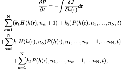where h(r) is the membrane height as a function of r = (x, y) and n_α is the number of monomers in the α^th filament. H(h(r), n_α) is the function that determines if there is sufficient space between the F-actin and the membrane for the addition of another monomer. If h(r) > n_αΔ, then H = 1; otherwise, H = 0. The intrinsic membrane flux, J, is defined as

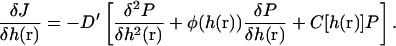(C3)

The definitions of φ and C are

(C4)

(C5)

E is the energy functional of Eq. 1 plus a term due to the presence of the actin filament and possible external forces F′,

(C6)

Here, U is the potential between the actin bundle tip and the plasma membrane. Equation C3 is the functional generalization of the ordinary Smoluchowski equation (56), the derivation of which will be given in a separate publication.

The interaction potential, U, is determined by the protrusion mechanism. For the Brownian ratchet model, U is a hardcore potential determined by the membrane position, h(r), and the heights of the filaments, n_αΔ. If h(r) > n_αΔ, then U = 0; otherwise, U = ∞. If there is a tether (Ena/VASP or other proteins) between the membrane tip and the membrane, then U is modified slightly: If h(r) > n_αΔ, then otherwise, U = ∞. All of the filaments interact with the membrane, thus we assume all the filaments are tethered. The tether elastic constant, κ_t, is a property of the tethering protein and an unknown parameter.

To solve the functional equation of Eq. C3, the membrane surface, h(r), is discretized into a set of small membrane elements. We work in the Cartesian coordinate system and, therefore, each membrane element has coordinates (x_i, y_j, h(x_i, y_j)). The membrane fluctuates by changing h_ij = h(x_i, y_j). The diffusion constant, D′, therefore describes the diffusing characteristics of each membrane element. The position of the membrane cap, z, is defined as

(C7)

where M is the number of membrane points in the cap. Since the transverse diffusion constant of a platelike object is proportional to its linear dimension, the relationship of Eq. 8 emerges.

APPENDIX D: MONTE CARLO SOLUTION ALGORITHM

The Fokker-Planck equations of Eqs. B1 and C3 are difficult to solve in closed form. Instead, we devised a Monte Carlo algorithm to generate trajectories of the moving system. The trajectories are averaged to obtain the reported results.

The algorithm is best explained in the context of Eq. B1. The one-dimensional variable, z, is discretized into small intervals. If the intervals are small enough, then a local steady-state approximation is valid and a local solution of the Fokker-Planck equation can be obtained for the interval. From this local solution, fluxes and transition rates to the neighboring intervals can be obtained (57). We find

(D1)

where k_± is the transition rate from z_i to z_i ± Δz, respectively. The transition rates satisfy the condition of detailed balance. The dynamic evolution of the system can be considered as a Markov process where the addition and subtraction of the monomers, and the movement of z, are the possible Markov transitions. Again, the procedure is valid when Δz is sufficiently small. In our calculations, Δz = Δ/N where Δ = 2.8 nm.

Combining all the possible transitions, the master equation of the composite system of filaments and the membrane cap can be written as

(D2)

where σ labels the composite state of the actin/membrane system as σ = (i,n₁,…,n_N), and P(σ) is the probability of the system to be in state σ. Likewise, M is the composite transition-probability matrix whose rate constants are given as k₁, k₂, and k_±. The nonzero elements of M are

• Addition of a monomer: If σ = (i,n₁,…,n_α,…,n_N) and σ′ = (i,n₁,…,n_α−1,…,n_N), and if the distance between the filament tip and z_i is >Δ, then M_{σ, σ′} = k₁; else, M_{σ, σ′} = 0.

• Loss of a monomer: If σ = (i,n₁,…,n_α,…,n_N) and σ′ = (i,n₁,…,n_α−1,…,n_N), then M_{σ, σ′} = k₂.

• Fluctuation of the membrane cap from z_i to z_i+1: If σ = (i,n₁,…,n_N) and σ′ = (i + 1,n₁,…,n_N), then M_{σ, σ′} = k₊; else M_{σ, σ′} = 0.

• Fluctuation of the membrane cap from z_i to z_i–1: If σ = (i,n₁,…,n_N) and σ′ = (i − 1,n₁,…,n_N), and if z_i–1 is not less than any of the filament height, then M_{σ, σ′} = k_–; else M_{σ, σ′} = 0.

These definitions completely specify the matrix M.

To generalize this procedure to Eq. C3, we discretize the membrane surface, as well as the membrane height, h(r). Thus, the membrane is a surface in a three-dimensional grid, (i, j, k). If Δh is small enough, the same local steady-state approximation applies. The transition rates between k and k ± 1 are

(D3)

where E is the membrane energy of Eq. C6. The composite state of the system is now labeled as σ = (i,j,k,n₁,…,n_N). The elements of the transition matrix are given by

• Addition of a monomer: If σ = (i,j,k,n₁,…,n_α,…,n_N) and σ′ = (i,j,k,n₁,…,n_α+1,…,n_N), and if the distance between the filament tip and h_k(i, j) is >Δ, then M_{σ, σ′} = k₁; else, M_{σ, σ′} = 0.

• Loss of a monomer: If σ = (i,j,k,n₁,…,n_α,…,n_N) and σ′ = (i,j,k,n₁,…,n_α−1,…,n_N), then M_{σ, σ′} = k₂.

• Fluctuation of the membrane cap from h_k(i, j) to h_k+1(i, j): If σ = (i,j,k,n₁,…,n_N) and σ′ = (i′,j′,k+1,n₁,…,n_N), and if h_k+1(i′, j′) is not less than any of the filament height, then M_{σ, σ′} = k₊δ_{i, i′}δ_{j, j′}; else M_{σ, σ′} = 0.

• Fluctuation of the membrane cap from z_i to z_i–1: If σ = (i,j,k,n₁,…,n_N) and σ′ = (i′,j′,k−1,n₁,…,n_N), and if h_k–1(i′, j′) is not less than any of the filament height, then M_{σ, σ′} = k_–δ_{i, i′}δ_{j, j′}; else M_{σ, σ′} = 0.

These definitions completely specify the Markov dynamics of the membrane and the filament growth.

In principle, it is possible to solve the Markov equation of Eq. D2 by finding the eigenvalues and eigenvectors of the transition matrix. However, the dimension of M is extremely large. Instead, Monte Carlo importance sampling of representative trajectories is more appropriate. The algorithm of Bortz, Kalos, and Lebowitz can accomplish this (58). Given a current state σ at time t, all future destination-states (i.e., trajectories) can be found iteratively by this algorithm. Dynamical observable such as the protrusion length as a function of time can be expressed as the trajectory average,

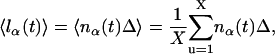(D4)

where the sum is over X number of repeated trajectories. To compute the trajectories, the following procedure is followed:

• For the current state, σ, find 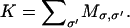K is then the rate of leaving the current state. Define a sequence of intervals between 0 and K. The intervals are given by the transition rate constants, M_{σ, σ′}. Note that many of the transition rates are zero. The identity of the destination state, σ′, is still unknown.

• Choose a random number, r, such that 0 < r < K.

• Find which interval r falls between 0 and K. This defines the destination state, σ′.

• Choose another random number, r′, between 0 and 1 and compute dt = −log(r′)/K. The value dt is the time elapsed during the change of state.

• Update the time to t = t + dt and the current state to σ′.

• Repeat the procedure.

By repeating the algorithm given above, all possible dynamical changes in the system are sampled. The algorithm is a form of importance sampling where the likely trajectories appear more frequently according to their statistical weight in trajectory space. All computational results in the article are obtained using this procedure.

Although adding membrane flexibility to the model revealed many interesting effects, we note that the computational cost incurred is substantial, especially when D′ is large. In this regime, most of the computer time is used to simulate membrane movement, and polymerization events are rare. In Fig. 6 a, protrusion velocities, when D′ > 10⁶ nm²/s, are difficult to obtain.

References

- 1.Pollard, T. D., L. Blanchoin, and R. D. Mullins. 2000. Molecular mechanisms controlling actin filaments dynamics in nonmuscle cells. Annu. Rev. Biophys. Biomol. Struct. 29:545–576. [DOI] [PubMed] [Google Scholar]
- 2.Borisy, G. G., and T. M. Svitkina. 2000. Actin machinery: pushing the envelope. Curr. Opin. Cell Biol. 12:104–112. [DOI] [PubMed] [Google Scholar]
- 3.Small, J. V. 1988. The actin cytoskeleton. Electron Microsc. Rev. 1:155–174. [DOI] [PubMed] [Google Scholar]
- 4.Lewis, A. K., and P. C. Bridgman. 1992. Nerve growth cone lamellipodia contain two populations of actin filaments that differ in organization and polarity. J. Cell Biol. 119:1219–1243. [DOI] [PMC free article] [PubMed] [Google Scholar]
- 5.Svitkina, T. M., E. A. Bulanova, O. Y. Chaga, D. M. Vignevic, S. Kojima, J. M. Vasiliev, and G. G. Borisy. 2003. Mechanism of filopodia initiation by reorganization of dendritic network. J. Cell Biol. 160:409–421. [DOI] [PMC free article] [PubMed] [Google Scholar]
- 6.Svitkina, T. M., and G. G. Borisy. 1999. Progress in protrusion: the tell-tale scar. Trends Biochem. Sci. 24:432–436. [DOI] [PubMed] [Google Scholar]
- 7.Mejillano, M. R., S. Kojima, D. A. Applewhite, F. B. Gertler, T. M. Svitkina, and G. G. Borisy. 2004. Lamellipodial versus filopodial mode of the actin nanomachinery: pivotal role of the filament barbed end. Cell. 118:363–373. [DOI] [PubMed] [Google Scholar]
- 8.Small, V. J., T. Stradal, E. Vignal, and K. Rottner. 2002. The lamellipodium: where motility begins. Trends Cell Biol. 12:112–119. [DOI] [PubMed] [Google Scholar]
- 9.Forscher, P., C. H. Lin, and C. Thompson. 1992. Novel form of cone motility site-directed actin filament assembly. Nature. 357:515–518. [DOI] [PubMed] [Google Scholar]
- 10.Peskin, C., G. Odell, and G. Oster. 1993. Cellular motions and thermal fluctuations: the Brownian ratchet. Biophys. J. 65:316–324. [DOI] [PMC free article] [PubMed] [Google Scholar]
- 11.Svitkana, T. M., E. A. Bulanova, O. Y. Chana, D. M. Vignjevic, S. Kojima, J. M. Vasiliev, and G. G. Borisy. 2003. Mechanism of filopodia initiation by reorganization of a dendritic network. J. Cell Biol. 160:409–421. [DOI] [PMC free article] [PubMed] [Google Scholar]
- 12.Vignjevic, D., D. Yarar, M. D. Welch, J. Peloquin, T. M. Svitkana, and G. G. Borisy. 2003. Formation of filopodia-like bundles in vitro from a dendritic network. J. Cell Biol. 160:951–962. [DOI] [PMC free article] [PubMed] [Google Scholar]
- 13.Tseng, Y., E. Fedorov, J. M. McCaffery, S. C. Almo, and D. Wirtz. 2001. Micromechanics and microstructure of actin filament networks in the presence of the actin-bundling protein human Fascin: a comparison with α-actinin. J. Mol. Biol. 310:351–366. [DOI] [PubMed] [Google Scholar]
- 14.Kureishy, N., V. Sapountzi, S. Prag, N. Anilkumar, and J. C. Adams. 2002. Fascins, and their roles in cell structure and function. Bioassays. 24:350–361. [DOI] [PubMed] [Google Scholar]
- 15.Jawhari, A. U., A. Buda, M. Jenkins, K. Shehzad, C. Sarraf, M. Noda, M. J. Farthing, M. Pignatelli, and J. C. Adams. 2003. Fascin, an actin-bundling protein, modulates colonic epithelial cell invasiveness and differentiation in vitro. Am. J. Pathol. 162:69–80. [DOI] [PMC free article] [PubMed] [Google Scholar]
- 16.Tseng, Y., K. M. An, O. Esue, and D. Wirtz. 2004. The bimodal role of filamin in controlling the architecture and mechanics of F-actin networks. J. Biol. Chem. 279:1819–1826. [DOI] [PubMed] [Google Scholar]
- 17.Kole, T. P., Y. Tseng, I. Jiang, J. L. Katz, and D. Wirtz. 2005. Intracellular mechanics of migrating fibroblasts. Mol. Biol. Cell. 16:328–338. [DOI] [PMC free article] [PubMed] [Google Scholar]
- 18.Mallavarapu, A., and T. Mitchison. 1999. Regulated actin cytoskeleton assembly at filopodium tips controls their extension and retraction. Semin. Cell Biol. 5:157–163. [DOI] [PMC free article] [PubMed] [Google Scholar]
- 19.Steketee, M. B., and K. W. Tosney. 2002. Three functionally distinct adhesions in filopodia: shaft adhesions control lamellar extension. J. Neurosci. 22:8071–8083. [DOI] [PMC free article] [PubMed] [Google Scholar]
- 20.Lanier, L. M., M. A. Gates, W. Witke, A. S. Menzies, A. M. Wehman, J. D. Macklis, D. Kwiatkowski, P. Soriano, and F. B. Gertler. 1999. Mena is required for neurulation commissure formation. Neuron. 22:313–325. [DOI] [PubMed] [Google Scholar]
- 21.Rottner, K., B. Behrendt, J. V. Small, and J. Wehland. 1999. VASP dynamics during lamellipodia protrusion. Nat. Cell Biol. 1:321–322. [DOI] [PubMed] [Google Scholar]
- 22.Mogilner, A., and G. Oster. 1996. Cell motility driven by actin polymerization. Biophys. J. 71:3030–3045. [DOI] [PMC free article] [PubMed] [Google Scholar]
- 23.Kovar, D. R., and T. D. Pollard. 2004. Insertional assembly of actin filament barbed ends in association with formin produces picoNewton forces. Proc. Natl. Acad. Sci. USA. 101:14725–14730. [DOI] [PMC free article] [PubMed] [Google Scholar]
- 24.Mogilner, A., and G. Oster. 1996. The physics of lamellipodial protrusion. Eur. Biophys. J. 25:47–53. [Google Scholar]
- 25.Grimm, H. P., A. B. Verkhovsky, A. Mogilner, and J.-J. Meister. 2003. Analysis of actin dynamics at the leading edge of crawling cells: implications for the shape of keratocyte lamellipodia. Eur. Biophys. J. 32:563–577. [DOI] [PubMed] [Google Scholar]
- 26.Carlsson, A. E. 2001. Growth of branched network against obstacles. Biophys. J. 81:1907–1923. [DOI] [PMC free article] [PubMed] [Google Scholar]
- 27.Mogilner, A., and B. Rubinstein. 2005. The physics of filopodial protrusion. Biophys. J. 89:1–14. [DOI] [PMC free article] [PubMed] [Google Scholar]
- 28.van Doorn, G. S., C. Tanase, B. M. Mulder, and M. Dogterom. 2000. On the stall force for growing microtubules. Eur. Biophys. J. 29:2–6. [DOI] [PubMed] [Google Scholar]
- 29.Stukalin, E. B., and A. B. Kolomeisky. 2005. Polymerization dynamics of double-stranded biopolymers: chemical kinetic approach. J. Chem. Phys. 122:104903. [DOI] [PubMed] [Google Scholar]
- 30.Stukalin, E. B., and A. B. Kolomeisky. 2004. Simple growth models of rigid multifilament biopolymers. J. Chem. Phys. 121:1097–1104. [DOI] [PubMed] [Google Scholar]
- 31.Canham, P. 1970. The minimum of the energy of bending as a possible explanation of the biconcave shape of the human red blood cell. J. Theor. Biol. 26:61–81. [DOI] [PubMed] [Google Scholar]
- 32.Helfrich, W. 1973. Elastic properties of lipid bilayers: theory and possible experiments. Z. Naturforsch. Z. Naturforsch. C. 28:693–703. [DOI] [PubMed] [Google Scholar]
- 33.Powers, T. R., G. Huber, and R. E. Goldstein. 2002. Fluid membrane tethers: minimum surfaces and elastic boundary layers. Phys. Rev. E. 65:041901. [DOI] [PubMed] [Google Scholar]
- 34.Derenyi, I., F. Julicher, and J. Prost. 2002. Formation and interaction of membrane tubes. Phys. Rev. Lett. 88:238101. [DOI] [PubMed] [Google Scholar]
- 35.Evans, E., and W. Rawicz. 1990. Entropy-driven tension and bending elasticity in condensed-fluid membranes. Phys. Rev. Lett. 64:2094–2097. [DOI] [PubMed] [Google Scholar]
- 36.Dai, J., and M. P. Sheetz. 1999. Membrane tether formation from blebbing cells. Biophys. J. 77:3363–3370. [DOI] [PMC free article] [PubMed] [Google Scholar]
- 37.Landau, L., and E. M. Lifshitz. 1986. Theory of Elasticity, 3rd Ed. Butterworth-Heinemann, Boston, MA.
- 38.Gittes, F., B. Mickey, J. Nettleton, and J. Howard. 1993. Flexural rigidity of microtubules and actin filaments measured from thermal fluctuations in shape. J. Cell Biol. 120:923–934. [DOI] [PMC free article] [PubMed] [Google Scholar]
- 39.Dembo, M. 1986. Mechanics and control of the cytoskeleton in Amoeba proteus. Biophys. J. 55:1053–1080. [DOI] [PMC free article] [PubMed] [Google Scholar]
- 40.Fushimi, K., and J. Theriot. 1991. Low viscosity in the aqueous domain of cell cytoplasm measured by picosecond polarization microfluorimetry. J. Cell Biol. 112:719–725. [DOI] [PMC free article] [PubMed] [Google Scholar]
- 41.Valberg, P. A., and H. A. Feldman. 1987. Magnetic particle motions within living cells. Measurement of cytoplasmic viscosity and motile activity. Biophys. J. 52:551–561. [DOI] [PMC free article] [PubMed] [Google Scholar]
- 42.Kole, T. P., Y. Tseng, L. Huang, J. L. Katz, and D. Wirtz. 2004. Rho kinase regulates the micromechanical response of adherent cells to Rho activation. Mol. Biol. Cell. 15:3475–3484. [DOI] [PMC free article] [PubMed] [Google Scholar]
- 43.Marchand, J.-B., P. Moreau, A. Paoletti, P. Cossart, M. F. Carlier, and D. Pantaloni. 1995. Actin-based movement of Listeria monocytogenes: actin assembly results from the local maintenance of the uncapped filament barbed ends at the bacterium surface. J. Cell Biol. 130:331–343. [DOI] [PMC free article] [PubMed] [Google Scholar]
- 44.Soo, F. S., and J. A. Theriot. 2005. Large-scale quantitative analysis of sources of variation in actin polymerization-based movement in Listeria monocytogenes. Biophys. J. 89:703–723. [DOI] [PMC free article] [PubMed] [Google Scholar]
- 45.Atilgan, E., D. Wirtz, and S. X. Sun. 2005. Morphology of the lamellipodium and the organization of actin at the leading edge of crawling cells. Biophys. J. 89:3589–3602. [DOI] [PMC free article] [PubMed] [Google Scholar]
- 46.Pollard, T. D., and G. G. Borisy. 2003. Cellular motility driven by actin assembly and disassembly of actin filaments. Cell. 112:453–465. [DOI] [PubMed] [Google Scholar]
- 47.Dickinson, R. B., L. Caro, and D. L. Purich. 2004. Force generation by cytoskeletal filament end-tracking proteins. Biophys. J. 87:2838–2854. [DOI] [PMC free article] [PubMed] [Google Scholar]
- 48.Kozlov, M. M., and A. D. Bershadsky. 2004. Processive capping by formin suggests a force-driven mechanism of actin polymerization. J. Cell Biol. 167:1011–1017. [DOI] [PMC free article] [PubMed] [Google Scholar]
- 49.Nelson, D., T. Piran, and S. Weinberg (editors). 2004. Statistical Mechanics of Membranes and Surfaces, 2nd Ed. World Scientific, Singapore.
- 50.Kumar, P. B., G. Gomper, and R. Lipowsky. 2001. Budding dynamics of multicomponent membranes. Phys. Rev. Lett. 86:3911–3914. [DOI] [PubMed] [Google Scholar]
- 51.Julicher, F. 1996. Conformal degeneracy of vesicles. J. Phys. II France. 6:1797–1823. [Google Scholar]
- 52.Frenkel, D., and B. Smit. 2002. Understanding Molecular Simulation. Computational Science Series, 2nd Ed. Elsevier, Dordrecht, The Netherlands.
- 53.Pollard, T. D. 1986. Rate constants for the reaction of ATP- and ADP-actin with the ends of actin filaments. J. Cell Biol. 103:2747–2754. [DOI] [PMC free article] [PubMed] [Google Scholar]
- 54.Doi, M., and S. F. Edwards. 1986. The Theory of Polymer Dynamics. Clarendon Press, Oxford, UK.
- 55.Yeung, A., and E. Evans. 1995. Unexpected dynamics in shape fluctuations of bilayer vesicles. J. Phys. II France. 5:1501–1523. [Google Scholar]
- 56.Risken, H. 1996. The Fokker-Planck Equation, 2nd Ed. Springer-Verlag, Berlin.
- 57.Wang, H., C. S. Peskin, and T. C. Elston. 2003. A robust numerical algorithm for studying biomolecular transport processes. J. Theor. Biol. 221:491–511. [DOI] [PubMed] [Google Scholar]
- 58.Bortz, A., M. Kalos, and J. Lebowitz. 1975. A new algorithm for Monte Carlo simulation of spin systems. J. Comput. Phys. 17:10–18. [Google Scholar]