Slaving: Solvent fluctuations dominate protein dynamics and functions

Abstract

Protein motions are essential for function. Comparing protein processes with the dielectric fluctuations of the surrounding solvent shows that they fall into two classes: nonslaved and slaved. Nonslaved processes are independent of the solvent motions; their rates are determined by the protein conformation and vibrational dynamics. Slaved processes are tightly coupled to the solvent; their rates have approximately the same temperature dependence as the rate of the solvent fluctuations, but they are smaller. Because the temperature dependence is determined by the activation enthalpy, we propose that the solvent is responsible for the activation enthalpy, whereas the protein and the hydration shell control the activation entropy through the energy landscape. Bond formation is the prototype of nonslaved processes; opening and closing of channels are quintessential slaved motions. The prevalence of slaved motions highlights the importance of the environment in cells and membranes for the function of proteins.

… everything that living things do can be understood in terms of the jigglings and wigglings of atoms.

R. P. Feynman (1)

Proteins perform most of the functions of living things, from metabolism to thinking. Textbooks usually show proteins naked, neglect fluctuations, and take little notice of the protein environment. Real proteins, however, are wiggling and jiggling, dressed by the hydration shell, and embedded in a cell or cell membrane. Feynman (1) stated the central problem succinctly, namely understanding protein functions in terms of the atomic motions. We are still very far from this goal, but progress is being made. Here we consider the effect of solvent fluctuations on protein processes. We will show that protein motions can be nonslaved or slaved. Nonslaved motions are independent of the solvent fluctuations. Slaved motions have rates that are proportional to the fluctuation rate of the solvent, but are smaller. We introduce a model, based on the energy landscape of the protein, that suggests how the protein controls its slaved dynamics. We use myoglobin (Mb) as a prototype, but the concepts apply also to many other proteins.

The Dichotomy of Motions

The main result of the present article emerges when the temperature dependences of protein processes are compared with the dielectric relaxation rate coefficient k_diel(T) (2) of the solvent, essentially the average tumbling rate of the solvent water molecules. Fig. 1 shows k_diel(T) (2) and the rate coefficients for various processes in Mb embedded in a 3:1 (vol/vol) glycerol/water solvent (3–7). [We do not consider vibrations here, which can be described by normal modes (8).] We characterize the rate coefficients for selected processes by using the Inset in Fig. 1. The Inset shows a cross section through part of Mb with a heme group situated in the heme cavity and a major cavity called Xe-1 and labeled D. Small ligands such as carbon monoxide (CO) bind covalently at the heme iron. We denote the position of the CO by S if it is in the solvent, by A if it is bound covalently to the iron, by B if it is still in the heme pocket but not covalently bound (9–11), and by D (11–13) if it resides in the Xe-1 pocket. The rate coefficient for the covalent binding B → A is called k_BA(T) and the one for the escape from D into the solvent is called k_DS(T). Mb molecules can assume three different structures or taxonomic substates: A₀, A₁, and A₃ (5, 14–16). Fluctuations between these substates are denoted by k₀₁(T) and k₁₃(T). Fast fluctuations, observed for instance by vibrational echo experiments (17), are denoted by k_ff. Slower fluctuations, observed after spectral hole burning (18), are labeled k_fluct(T). The relaxations of the width and the position of the stretch frequency of the bound CO after a pressure release are described by the rate coefficient k_relax (14, 15).

Fig. 1.

The temperature dependence of selected rate coefficients in Mb. The rate coefficient for the dielectric fluctuations in the solvent (glycerol/water, 3:1 vol/vol) is denoted by k_diel (2, 7). (Inset) A cross section through part of Mb. In state A, not labeled, the CO ligand binds at the iron in the center of the heme group, shown in red. B indicates the site occupied by CO after dissociation from Fe, and D indicates the CO position in the Xe-1 cavity. The protein rate coefficients refer to binding of CO at the heme iron (k_BA) (3), exit into the solvent S (k_DS, ▪) (3, 7), equilibrium fluctuations after hole burning (k_fluct, ⧫) (18), and fluctuations among the taxonomic substates A₀, A₁, and A₃ (k₀₁, •; k₁₃, ▴) (15, 16). Some of the A-state relaxation data are from ref. 67. The rate coefficients for the shift of the center frequency and the width (pentagon, ▾) of the CO stretch band after a pressure change are denoted by k_relax (14, 15). The dephasing rate of the CO stretching mode of Mb-CO is denoted by k_ff (17).

Two classes of protein processes, nonslaved and slaved, emerge from an Arrhenius plot (Fig. 1). The two classes of processes are clearly distinguished in the plot of log(k/k_diel) in Fig. 2. Nonslaved processes, such as the geminate binding of the CO (k_BA) and the fast fluctuations (k_ff), have temperature dependences that are very different from k_diel(T). They follow Arrhenius relations with pre-exponential factors of the order of 10¹³ s⁻¹ or less. At least two different nonslaved processes exist. Some, like k_BA and k_ff, can be observed to far below 200 K. Other fast motions, observed by using the Mössbauer effect (19, 20) and neutron scattering (21) become unobservable below the protein glass (dynamic) transition, which in a 3:1 glycerol/water solvent occurs at about 170 K (5, 15). Slaved processes, such as the escape of the CO into the solvent (k_DS), and protein relaxations and fluctuations (A₀ ⇌ A₁, A₁ ⇌ A₃, k_relax, k_fluct), have approximately the same temperature dependence as k_diel, depend markedly on solvent viscosity, and are absent in a solid surrounding (3). Their temperature dependencies can be described by the Vogel–Fulcher equation, k(T) = Aexp[H/k_B(T − T₀)] (14). If fit to an Arrhenius relation, the pre-exponential factor can be much larger than 10¹³ s⁻¹ and the activation enthalpy is temperature dependent. Slaved processes can still have small internal (i.e., nonsolvent) enthalpy barriers, as exemplified by the ratio k_DS/k_diel in Fig. 2. This ratio has a small slope, corresponding to an internal activation barrier of about 10 kJ/mol, because CO is more tightly bound in D than S by about this amount. There may also be a small internal enthalpy barrier slowing entry and exit. Additional evidence for the solvent control of slaved transitions comes from comparing the rate coefficients k_DS in different solvents. Table 1 gives log k_DS, log k_diel, and log(k_DS/k_diel) in three different solvents at 220 K, by using data from Kleinert et al. (7). Although the dielectric relaxation rates differ by more than a factor of 1,000, the ratio k_DS/k_diel is unchanged. These results imply that the rate coefficient for a slaved transition can be written as

Here k(T) is the rate of a slaved process and n(T) is a coefficient indicating how much the protein, including the hydration shell, slows the effect of the solvent fluctuations. The coefficient k_diel(T) is a steep function of T (Fig. 1), whereas n(T) depends only weakly on T. The solvent thus dominates the activation enthalpy for slaved processes, whereas the protein controls the activation entropy. Fig. 2 shows that n(T) varies widely from one process to another. It is ≈10 for the pressure relaxation (k_relax), 10³ for equilibrium fluctuations after hole burning (k_fluct), 10⁴ for the exit of CO from Mb, and 10⁵ for fluctuations between A₀ and A₁. These observations raise two questions: How does the solvent influence the protein? How does the protein control the coefficient n(T)? We turn to the energy landscape to answer these questions.

Fig. 2.

Temperature dependence of the ratio (k/k_diel), where k stands for the rate coefficients of the processes shown in Fig. 1. The symbols are as in Fig. 1.

Table 1.

The ratio (k_DS/k_diel) for Mb in different solvents at 220 K

Solvent	log(kDS/s−1)	log(kdiel/s−1)	log(kDS/kdiel)
60% EW	3.1	8.2	−5.1
75% GW	0.7	6.0	−5.3
90% GW	−0.2	5.1	−5.3

The data are from Kleinert et al. (7). W, water; E, ethylene glycol; G, glycerol.

The Energy Landscape

Proteins and nucleic acids can assume a large number of different conformations called conformational substates (3, 22–25). A substate is specified by the coordinates of every atom of the protein and its hydration shell. The energy landscape thus is a construct in a high-dimensional conformation space, with ≈10⁴ coordinates. Substates are conformational minima, described by points in this space. The substates are organized into tiers characterized by the magnitude of the barriers between them. The top tier in Mb, with the largest barriers, is formed by three taxonomic substates, A₀, A₁, and A₃. The taxonomic substates are identified by the stretch frequencies, ν_CO, of CO bound to the heme iron. Their properties, for instance, structure, function, and reaction rates, can be determined individually (5, 26). A₁ dominates at high pH and stores dioxygen. A₀ dominates at low pH and is involved in NO enzymatics (27). The function of A₃, if any, is not known. Each taxonomic substate can assume a very large number of different conformations, mainly because of different orientations of amino acid side chains and conformations of the hydration shell. These protein conformations are called statistical substates because they are so numerous that they cannot be characterized individually. Within each statistical substate reside local conformational minima characterized by very small barriers (28).

Protein motions are jumps between substates (29). At temperatures well below 170 K in a 3:1 glycerol/water solvent only transitions between local conformational minima are observed (28). Above ≈170 K some very fast processes (k > 10⁹ s⁻¹ ≫ k_diel) are seen in inelastic neutron scattering and Mössbauer experiments (19–21). Slow slaved motions also become observable above ≈170 K (Fig. 1). At 170 K, the slaved rate coefficients are <10⁻⁴ s⁻¹. We interpret the very fast processes as transitions among local conformational minima and the slaved motions as jumps between statistical and between taxonomic substates. This situation is sketched in Fig. 3 (30). Fig. 3a shows three statistical substates as shallow craters within a small part of the energy landscape. The two coordinates fc1 and fc2 in Fig. 3 are not two coordinates of a particular atom, but are functionally relevant coordinates that describe individual steps (31). Within each crater there are many local minima, shown as small circles. Fig. 2 and Eq. 1 imply that the rate coefficients for slaved transitions are proportional to k_diel; for simplicity we assume that they are given by k_diel. At ≈170 K, a protein in a statistical substate fluctuates rapidly among the local minima and only every 10⁴ s or so jumps to another statistical substate. At physiological temperatures, however, transitions between statistical substates occur in <1 ns. The resulting dynamics is sketched in Fig. 3b, which represents an entire taxonomic substate. Each protein performs a random walk in the conformation space (32). A protein starting in a substate I can reach a substate F by a large number of different paths. Only a single realization of the many possible paths is shown in Fig. 3b. The model introduced here uses a Brownian motion in conformation space. An earlier model used a Brownian oscillator in real space to explain the temperature dependence of the mean-squared displacement at the position of the heme iron as observed by the Mössbauer effect (33).

Fig. 3.

2D cross sections through the energy landscape of Mb. The functional coordinates fc1 and fc2 describe the transitions between selected substates (31). (a) Cross section of a small part of the energy landscape. Three statistical substates are shown as shallow craters. The small circles inside the craters are local conformational minima. At temperatures well below 170 K, only transitions among the local conformational minima are observable. Above 170 K, jumps among statistical substates, induced by fluctuations in the solvent and shown as heavy arrows, become observable. (b) At 300 K, each protein performs a random walk in the conformation (energy) landscape. A walk that terminates at the black square opens a channel. A walk starting from an “excited” state describes a relaxation. The actual random walk is far more complex than shown here, because it occurs in a few thousand dimensions rather than the two shown here. The scales in a and b are very different. In a only a very small region in the conformational space is shown; b represents the entire space of a particular taxonomic substate.

Solvent Fluctuations Are Responsible for Slaving

Fluctuations permit conformational motions (34, 35), for instance, flips of the side chains and motions of the backbone, thus causing transitions among the substates (36). Slaving, the fact that many protein fluctuations occur with the temperature dependence of the solvent fluctuations, implies that the solvent fluctuations overwhelm the intrinsic fluctuations of the protein and the hydration shell. Fluctuations in the enthalpy H, the volume V, and the electric dipole moment M (37, 38) can be responsible for slaving. The fluctuations are given by the relevant susceptibilities, the heat capacity C_P at constant pressure, the isothermal bulk compressibility B_T, and the polarizability (dielectric susceptibility) χ (39):

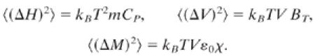Here k_B is the Boltzmann constant and ɛ₀ the permittivity coefficient of vacuum. V and m are volume and mass of the protein, respectively. The susceptibilities of solvents are larger than those of proteins: C_p for water is ≈4.2 J⋅K⁻¹⋅g⁻¹ and 1.3 J⋅K⁻¹⋅g⁻¹ for proteins; B_T is ≈4.5 × 10⁻¹⁰ Pa⁻¹ for water and ≈2 × 10⁻¹⁰ Pa⁻¹ for proteins. Most striking is the difference for χ = ɛ − 1, where ɛ is the dielectric coefficient. For water, as well as the hydration shell, ɛ is ≈80. Photon-echo experiments and calculations indicate that the protein itself, without the hydration shell, can be modeled as having a much smaller ɛ than the solvent (40–43). These data suggest that the electric dipole moment fluctuations are the dominant cause of the slaving. The fluctuating dipoles in the solvent interact with the dipoles in the hydration shell and with the charged side chains of the protein (44). Both the dipole–dipole and the dipole–charge interactions are long-ranged. Dipoles in a large volume of the solvent thus dominate the dipoles in the hydration shell. The fluctuations in the hydration shell and of the charged residues consequently are controlled by the solvent (45) and produce volume, enthalpy, and dielectric fluctuations in the protein. The hydration shell and the charged residues thus couple the protein to the surrounding thermal bath (46, 47).

The model can explain the slowing coefficient, n(T), the hierarchy of slaved processes without large internal enthalpy barriers, and the nonexponential time dependence of many slaved processes. Consider the random walk in Fig. 3b where the black square F represents, for instance, an open channel for the escape of a CO molecule. The time to exit through a channel is 1/k_DS. Because each step occurs in approximately a time 1/k_diel, the slowing coefficient n(T) is roughly equal to the number of steps necessary to reach the open channel substates, or n(T) = k_diel/k_DS (Eq. 1). The hierarchy of n(T) in Fig. 2 follows from structural considerations. The pressure used in the pressure relaxation experiments (15) produces only minor structural changes (48) and thus only a few steps are needed for the relaxation. Opening a channel for the entrance or exit of CO requires a larger structural change, explaining the larger value n(T) ∼ 10⁴. Fluctuations between A₀ and A₁ require two independent events, swinging in and out of His-64 and the presence of a solvated proton. Both events happen many times before a coincidence occurs, leading to n(T) ∼ 10⁵. Because the number of substates in the transition region between A₀ and A₁ is much smaller than the total number of statistical substates the protein barrier is entropic (49).

Slaved processes are often nonexponential in time (14, 15, 50) and can be described by a stretched exponential, exp{−(kt)^β}, β < 1, or a power law, (1 + κt)^−η.¶ Fig. 3b illustrates this effect as a complex increase in mean-squared displacement with time (homogeneous nonexponential behavior). Additionally, different structures of the protein will have different initial substates, I, and require different pathways to the final substate, F, with different times required for each path (inhomogeneous nonexponential behavior) (51, 52). The interplay between inhomogeneous and homogeneous contributions to protein dynamics has been observed experimentally (53, 54), and modeled in detail (55, 56). The fluctuation experiment of Shibata et al. (18), a pressure release experiment (15), and hole-burning experiments below 1 K (57) all give β ≈ 0.25, suggesting anomalous diffusion (58).

Slaving Occurs in Many Proteins

Mb has served as a test system for so many studies that it is important to ask whether the concepts that have emerged are valid also for other proteins. The answer is yes. A wide variety of proteins display slaved processes including separated hemoglobin chains (59), bacteriorhodopsin (60), leghemoglobin (61), azurin (62), the photosynthetic reaction center (63), dehydrogenases (64), catalase, phosphatase, and xylanese (65, 66).∥

Conclusions

Solvent motions dominate a broad range of protein processes, from conformational fluctuations and relaxations to ligand motions and catalysis. The solvent is an active participant and not an innocent bystander. Equally important is the protein energy landscape. Without the large number of statistical substates, the protein could not generate entropic barriers. The present approach, based on the rate of solvent fluctuations, provides more insight than the one based on the Kramers equation (4, 6, 7) because the rates for protein processes are compared directly to the rates of solvent fluctuations, without a detour involving viscosity. The results raise many questions. Mb is a small and not particularly flexible protein. How does slaving manifest itself in larger and multimeric proteins that execute large conformational motions, for instance, myosin? What is the energy landscape of a protein in vacuum? How do protein–protein and protein–RNA interactions affect the dynamics? What is the dielectric relaxation rate in membranes and cells? Do membranes and cells use the interaction between environment and protein to perform and control reactions? Is slaving involved in the functions of DNA and RNA? The answers to these questions may lead to a better understanding of how proteins work in the biological environment.

Abbreviations

• Mb, myoglobin

References

- 1.Feynman R. P., (1963) Six Easy Pieces (Addison–Wesley, Reading, MA), pp. 59.
- 2.Huck J. R., Noyel, G. A. & Jorat, L. J. (1988) IEEE Trans. Electr. Insul. 23, 627-638. [Google Scholar]
- 3.Austin R. H., Beeson, K. W., Eisenstein, L., Frauenfelder, H. & Gunsalus, I. C. (1975) Biochemistry 14, 5355-5373. [DOI] [PubMed] [Google Scholar]
- 4.Beece D., Eisenstein, D. L., Frauenfelder, H., Good, D., Marden, M. C., Reinisch, L., Reynolds, A. H., Sorensen, L. B. & Yue, K. T. (1980) Biochemistry 19, 5147-5157. [DOI] [PubMed] [Google Scholar]
- 5.Ansari A., Berendzen, J., Braunstein, D., Cowen, B. R., Frauenfelder, H., Hong, M. K., Iben, I. E. T., Johnson, J. B., Ormos, P., Sauke, T. B. & Scholl, R. (1987) Biophys. Chem. 26, 337-355. [DOI] [PubMed] [Google Scholar]
- 6.Ansari A., Jones, C. M., Henry, E. R., Hofrichter, J. & Eaton, W. A. (1994) Biochemistry 33, 5128-5145. [DOI] [PubMed] [Google Scholar]
- 7.Kleinert T., Doster, W., Leyser, H., Petry, W., Schwarz, V. & Settles, M. (1998) Biochemistry 37, 717-733. [DOI] [PubMed] [Google Scholar]
- 8.Melchers B., Knapp, E. W., Parak, F., Cordone, L., Cupane, A. & Leone, M. (1996) Biophys. J. 70, 2092-2099. [DOI] [PMC free article] [PubMed] [Google Scholar]
- 9.Schlichting I., Berendzen, J., Phillips, G. N., Jr. & Sweet, R. M. (1994) Nature 371, 808-812. [DOI] [PubMed] [Google Scholar]
- 10.Hartmann H., Zinser, S., Komninos, P., Schneider, R. T., Nienhaus, G. U. & Parak, F. (1996) Proc. Natl. Acad. Sci. USA 93, 7013-7016. [DOI] [PMC free article] [PubMed] [Google Scholar]
- 11.Ostermann A., Waschipky, R., Parak, F. G. & Nienhaus, G. U. (2000) Nature 404, 205-208. [DOI] [PubMed] [Google Scholar]
- 12.Chu K., Vojtechovsky, J., McMahon, B. H., Sweet, R. M., Berendzen, J. & Schlichting, I. (2000) Nature 403, 921-923. [DOI] [PubMed] [Google Scholar]
- 13.Srajer V., Ren, Z., Teng, T. Y., Schmidt, M., Ursby, T., Bourgeois, D., Pradervand, C., Schildkamp, W., Wulff, M. & Moffat, K. (2001) Biochemistry 40, 13802-13815. [DOI] [PubMed] [Google Scholar]
- 14.Iben I. E. T., Braunstein, D., Doster, W., Frauenfelder, H., Hong, M. K., Johnson, J. B., Luck, S., Ormos, P., Schulte, A., Steinbach, P. J. & Xie, A. H. (1989) Phys. Rev. Lett. 62, 1916-1919. [DOI] [PubMed] [Google Scholar]
- 15.Frauenfelder H., Alberding, N. A., Ansari, A., Braunstein, D., Cowen, B. R., Hong, M. K., Iben, I. E. T., Johnson, J. B., Luck, S., Marden, M. C. & Mourant, J. R. (1990) J. Phys. Chem. 94, 1024-1037. [Google Scholar]
- 16.Johnson J. B., Lamb, D. C., Frauenfelder, H., Müller, J. D., McMahon, B., Nienhaus, G. U. & Young, R. D. (1996) Biophys. J. 71, 1563-1573. [DOI] [PMC free article] [PubMed] [Google Scholar]
- 17.Rector K. D., Jiang, J. W., Berg, M. A. & Fayer, M. D. (2001) J. Phys. Chem. B 105, 1081-1092. [Google Scholar]
- 18.Shibata Y., Kurita, A. & Kushida, T. (1999) Biochemistry 38, 1789-1801. [DOI] [PubMed] [Google Scholar]
- 19.Keller H. & Debrunner, P. G. (1980) Phys. Rev. Lett. 45, 68-71. [Google Scholar]
- 20.Parak F., Knapp, E. W. & Kucheida, D. (1982) J. Mol. Biol. 161, 177-194. [DOI] [PubMed] [Google Scholar]
- 21.Doster W., Cusack, S. & Petry, W. (1989) Nature 337, 754-756. [DOI] [PubMed] [Google Scholar]
- 22.Frauenfelder H., Petsko, G. A. & Tsernoglou, D. (1979) Nature 280, 558-563. [DOI] [PubMed] [Google Scholar]
- 23.Frauenfelder H., Sligar, S. G. & Wolynes, P. G. (1991) Science 254, 1598-1603. [DOI] [PubMed] [Google Scholar]
- 24.Onuchic J. N. & Wolynes, P. G. (1993) J. Chem. Phys. 98, 2218-2224. [Google Scholar]
- 25.Ansari A., Berendzen, J., Bowne, S. F., Frauenfelder, H., Iben, I. E. T., Sauke, T. B., Shyamsunder, E. & Young, R. D. (1985) Proc. Natl. Acad. Sci. USA 82, 5000-5004. [DOI] [PMC free article] [PubMed] [Google Scholar]
- 26.Yang F. & Phillips, G. N., Jr. (1996) J. Mol. Biol. 256, 762-774. [DOI] [PubMed] [Google Scholar]
- 27.Frauenfelder H., McMahon, B. H., Austin, R. H., Chu, K. & Groves, J. T. (2001) Proc. Natl. Acad. Sci. USA 98, 2370-2374. [DOI] [PMC free article] [PubMed] [Google Scholar]
- 28.Thorn-Leeson D. T., Wiersma, D. A., Fritsch, K. & Friedrich, J. (1997) J. Phys. Chem. B 101, 6331-6340. [Google Scholar]
- 29.Kitao A., Hayward, S. & Gō, N. (1998) Proteins 33, 496-517. [DOI] [PubMed] [Google Scholar]
- 30.Fritsch K. & Friedrich, J. (1997) Physica D 107, 218-224. [Google Scholar]
- 31.García A. E. & Hummer, G. (1999) Proteins 36, 175-191. [PubMed] [Google Scholar]
- 32.Bryngelson J. D. & Wolynes, P. G. (1989) J. Phys. Chem. 93, 6902-6915. [Google Scholar]
- 33.Knapp E. W., Fischer, S. F. & Parak, F. (1982) J. Phys. Chem. 86, 5042-5047. [Google Scholar]
- 34.Careri G., Fasella, P. & Gratton, E. (1975) CRC Crit. Rev. Biochem. 3, 141-164. [DOI] [PubMed] [Google Scholar]
- 35.Cooper A. (1984) Prog. Biophys. Mol. Biol. 34, 181-214. [DOI] [PubMed] [Google Scholar]
- 36.Eisenmesser E. Z., Bosco, D. A., Akke, M. & Kern, D. (2002) Science 295, 1520-1523. [DOI] [PubMed] [Google Scholar]
- 37.Dachwitz E., Parak, F. & Stockhausen, M. (1989) Ber. Bunsen-Ges. Phys. Chem. 93, 1454-1458. [Google Scholar]
- 38.Chang I., Hartmann, H., Krupyanskii, Y., Zharikov, A. & Parak, F. (1996) Chem. Phys. 212, 221-229. [Google Scholar]
- 39.Callen H. B., (1985) Thermodynamics and an Introduction to Thermostatistics (Wiley, New York).
- 40.Warshel A. & Aqvist, J. (1991) Annu. Rev. Biophys. Biophys. Chem. 20, 267-298. [DOI] [PubMed] [Google Scholar]
- 41.Voges D. & Karshikoff, A. (1998) J. Chem. Phys. 108, 2219-2227. [Google Scholar]
- 42.Jordanides X. J., Lang, M. J., Song, X. Y. & Fleming, G. R. (1999) J. Phys. Chem. B 103, 7995-8005. [Google Scholar]
- 43.Cohen B. E., McAnaney, T. B., Park, E. S., Jan, Y. N., Boxer, S. G. & Jan, L. Y. (2002) Science 296, 1700-1703. [DOI] [PubMed] [Google Scholar]
- 44.Bizzarri A. R. & Cannistraro, S. (2002) J. Phys. Chem. B 106, 6617-6633. [Google Scholar]
- 45.Singh G. P., Parak, F., Hunklinger, S. & Dransfeld, K. (1981) Phys. Rev. Lett. 47, 685-688. [Google Scholar]
- 46.Careri G. & Gratton, E. (1977) BioSystems 8, 185-186. [DOI] [PubMed] [Google Scholar]
- 47.Pal S. K., Peon, J. & Zewail, A. H. (2002) Proc. Natl. Acad. Sci. USA 99, 1763-1768. [DOI] [PMC free article] [PubMed] [Google Scholar]
- 48.Urayama P., Phillips, G. N., Jr. & Gruner, S. M. (2002) Structure (London) 10, 51-60. [DOI] [PubMed] [Google Scholar]
- 49.Zhou H.-X. & Zwanzig, R. (1991) J. Chem. Phys. 94, 6147-6152. [Google Scholar]
- 50.Jackson T. A., Lim, M. & Anfinrud, P. A. (1994) Chem. Phys. 180, 131-140. [Google Scholar]
- 51.Xia X. Y. & Wolynes, P. G. (2001) Phys. Rev. Lett. 86, 5526-5529. [DOI] [PubMed] [Google Scholar]
- 52.Hänggi P., Talkner, P. & Borkovec, M. (1990) Rev. Mod. Phys. 62, 251-341. [Google Scholar]
- 53.Post F., Doster, W., Karvounis, G. & Settles, M. (1993) Biophys. J. 64, 1833-1842. [DOI] [PMC free article] [PubMed] [Google Scholar]
- 54.Tian W. D., Sage, J. T., Champion, P. M., Chien, E. & Sligar, S. G. (1996) Biochemistry 35, 3487-3502. [DOI] [PubMed] [Google Scholar]
- 55.Wang J. & Wolynes, P. (1994) Chem. Phys. 180, 141-156. [Google Scholar]
- 56.Wang J. & Wolynes, P. (1996) J. Phys. Chem. 100, 1129-1136. [Google Scholar]
- 57.Schlichter J., Fritsch, K.-D., Friedrich, J. & Vanderkooi, J. M. (1999) J. Chem. Phys. 110, 3229-3234. [Google Scholar]
- 58.Zeldovich Ya. B., Ruzmaikin, A. A. & Sokoloff, D. D., (1990) The Almighty Chance (World Scientific, Teaneck, NJ).
- 59.Alberding N., Chan, S. S., Eisenstein, I., Frauenfelder, H., Good, D., Gunsalus, I. C., Nordlund, T. M., Perutz, M. F., Reynolds, A. H. & Sorensen, L. B. (1978) Biochemistry 17, 43-50. [DOI] [PubMed] [Google Scholar]
- 60.Beece D., Browne, S. F., Czégé, J., Eisenstein, L., Frauenfelder, H., Good, D., Marden, M. C., Marque, J., Ormos, P., Reinisch, L. & Yue, K. T. (1981) Photochem. Photobiol. 33, 517-522. [Google Scholar]
- 61.Stetzkowski F., Banerjee, R., Marden, M. C., Beece, D. K., Bowne, S. F., Doster, W., Eisenstein, L., Frauenfelder, H. & Reinisch, L. (1985) J. Biol. Chem. 260, 8803-8809. [PubMed] [Google Scholar]
- 62.Ehrenstein D. & Nienhaus, G. U. (1992) Proc. Natl. Acad. Sci. USA 89, 9681-9685. [DOI] [PMC free article] [PubMed] [Google Scholar]
- 63.McMahon B. H., Müller, J. D., Wraight, C. A. & Nienhaus, G. U. (1998) Biophys. J. 74, 2567-2587. [DOI] [PMC free article] [PubMed] [Google Scholar]
- 64.Demchenko A. P., Rusyn, O. I. & Saburova, E. A. (1989) Biochem. Biophys. Acta 998, 196-203. [DOI] [PubMed] [Google Scholar]
- 65.Daniel R. M., Smith, J. C., Ferrand, M., Héry, S., Dunn, R. & Finney, J. L. (1998) Biophys. J. 75, 2504-2507. [DOI] [PMC free article] [PubMed] [Google Scholar]
- 66.Dunn R. V., Reat, V., Finney, J., Ferrand, M., Smith, J. C. & Daniel, R. M. (2000) Biochem. J. 346, 355-358. [PMC free article] [PubMed] [Google Scholar]
- 67.Scholl R. W., (1991) Ph.D. thesis (Univ. of Illinois, Urbana-Champaign).