

Abstract
The neural mechanism that mediates perceptual filling-in of the blind spot is still under discussion. One hypothesis proposes that the cortical representation of the blind spot is activated only under conditions that elicit perceptual filling-in, and requires congruent stimulation on both sides of the blind spot. Alternatively, the passive remapping hypothesis proposes that inputs from regions surrounding the blind spot infiltrate the representation of the blind spot in cortex. This theory predicts that independent stimuli presented to the left and right of the blind spot should lead to neighboring/overlapping activations in visual cortex when the blind-spot eye is stimulated, but separated activations when the fellow eye is stimulated. Using functional MRI, we directly tested the remapping hypothesis by presenting flickering checkerboard wedges to the left or right of the spatial location of the blind spot, either to the blind-spot eye or to the fellow eye. Irrespective of which eye was stimulated, we found separate activations corresponding to the left and right wedges. We identified the centroid of the activations on a cortical flat map and measured the distance between activations. Distance measures of the cortical gap across the blind spot were accurate and reliable (mean distance 6-8 mm across subjects, SD ~1 mm within subjects). Contrary to the predictions of the remapping hypothesis, cortical distances between activations to the two wedges were equally large for the blind-spot eye and fellow eye in areas V1 and V2/V3. Remapping therefore appears unlikely to account for perceptual filling-in at an early cortical level.
Keywords: visual perception, visual cortex, filling-in, perceptual closure, neuronal plasticity, brain mapping, fMRI, magnetic resonance imaging
INTRODUCTION
The blind spot refers to the region where the optic nerve exits the eye. This special region does not contain any photoreceptors to detect visual information from the world around us. Despite the absence of visual information from this region of the eye, we rarely notice a ‘hole’ in the visual field during monocular vision. Rather, vision almost always seems complete. This phenomenon of perceptual filling-in seems to occur automatically at a pre-attentive level of visual processing (Ramachandran 1992b). However, perceptual filling-in of the blind spot occurs only under certain circumstances. Psychophysical studies have revealed that the presence of spatiotemporally coherent elements on both sides of the blind spot—elements that likely reflect a single unified object—is the main prerequisite for perceptual filling-in (Walls 1954). Once this criterion is fulfilled, the blind spot can be perceptually filled-in with uniform background colors, geometric patterns, and discrete stimuli that cross the blind spot (Ramachandran 1992a).
There have been several proposals regarding what type of mechanism mediates perceptual filling-in of the blind spot (Dennett 1991; Pessoa et al. 1998; Ramachandran 1992a; Tripathy et al. 1996; Walls 1954). One hypothesis, which we refer to as the active completion hypothesis, proposes that perceptual filling-in results from the propagation of visual information from neurons that represent the region surrounding the blind spot to neurons that represent the blind-spot region itself. According to this hypothesis, neuronal filling-in only occurs for stimuli that also lead to perceptual filling-in, namely during congruent stimulation on opposing sides of the blind spot (Fiorani et al. 1992). When only a single side of the blind-spot surround is stimulated, perceptual filling-in fails to occur, presumably because neural activity remains restricted to the stimulated region and fails to propagate into the cortical representation of the blind spot.
An alternative account is the passive remapping hypothesis, which proposes that visual inputs from the retinal region surrounding the blind spot are displaced such that they infiltrate cortical regions that would have normally represented the blind spot. According to the remapping hypothesis, stimuli presented to one side of the blind spot, which do not induce perceptual filling-in, should still lead to cortical activations that extend into the cortical representation of the blind spot (Chino et al. 2001). As a result, the hole corresponding to the retinal blind spot is effectively sewn-up in cortex, such that inputs from opposite sides of the blind spot project to adjacent regions in cortex. A final theory is that perceptual filling-in does not involve any type of neuronal filling-in; the brain simply ignores the absence of information from the blind-spot region (Andrews and Campbell 1991; Dennett 1991; Durgin et al. 1995). However, neurophysiological studies suggest that the strong version of this theory is unlikely to be true.
Single-unit recordings in the primary visual cortex (V1) of monkeys demonstrate partial neuronal filling-in of the blind spot. About a quarter of the neurons recorded in the V1 representation of the blind spot can be reliably excited by stimuli presented to the blind-spot eye, though most of these neurons still respond more strongly to stimulation of the fellow (non-blind-spot) eye (Fiorani et al. 1992; Komatsu et al. 2000; Matsumoto and Komatsu 2005). The response of these neurons to stimuli presented near the border of the blind spot may reflect active neural completion, passive remapping of inputs towards the representation of the blind spot in cortex, or non-specific spreading (i.e., blurring) of projections from retina to cortex. Most of the neurons that remain responsive to the blind-spot eye have unusually large bilateral receptive fields that exceed the size of the blind spot itself (Komatsu et al. 2000), indicating that these neurons receive diffuse input. Interestingly, a subset of these neurons show evidence of enhanced activity when opposite sides of the blind spot are stimulated at the same time, suggesting some degree of active neural completion (Fiorani et al. 1992; Matsumoto and Komatsu 2005). However, there is other evidence to suggest that passive remapping might also contribute to neuronal filling-in. When a long bar stimulus was used to map the receptive fields of V1 neurons, receptive-field centers for the blind-spot eye showed somewhat greater displacement towards the center of the blind spot, as compared to the fellow eye (Fiorani et al. 1992; but see also Komatsu et al., 2000). These findings could potentially reflect the effects of passive remapping. Most studies of cortical reorganization have focused on the effects of retinal lesions in the normal visual field. Small bilateral retinal lesions can dramatically alter the receptive fields of V1 neurons corresponding to the lesioned area; these neurons can acquire new receptive fields adjacent to the lesioned visual-field location (Gilbert and Wiesel 1992; Kaas et al. 1990). Functional imaging studies have reported similar cortical remapping effects after bilateral loss of retinal input in humans (Baker et al. 2005; Baseler et al. 2002). Recent studies indicate that monocular retinal lesions may also lead to the selective displacement of the receptive fields for the lesioned eye (Calford et al. 1999; Calford et al. 2000; Schmid et al. 1996), especially if the lesions occur early in development and are followed by a long period of recovery (Chino et al. 2001). However, other studies have failed to observe topographic remapping effects in V1 after monocular retinal lesions (Murakami et al. 1997) or even after bilateral retinal lesions in adult monkeys (Smirnakis et al. 2005). In summary, there is mixed evidence regarding whether monocular retinal lesions consistently lead to passive remapping, and it remains unclear if remapping occurs in the case of monocular loss of input at the blind spot.
Here, we used functional magnetic resonance imaging (fMRI) to map the cortical representation of space around the blind spot in order to test for passive remapping in early visual areas. Activation maps obtained with fMRI have been shown to closely agree with the maps obtained from independent measures of multi-unit activity and local field potentials (Smirnakis et al. 2005). By using fMRI, it is possible to investigate the underlying mechanisms of neuronal filling-in of the blind spot in multiple visual areas. Previous fMRI studies have shown that there is a weakly responsive region in V1, corresponding to the cortical representation of the blind spot, that is no longer evident in area V2 (Tong and Engel 2001; Tootell et al. 1998). These findings suggest that there may be stronger neuronal filling-in in extrastriate areas, but few if any studies have systematically investigated filling-in of the blind spot in areas beyond V1.
According to the passive remapping hypothesis, the cortical representation of visual locations surrounding the blind spot should differ in topography for the blind-spot eye and the fellow eye, with remapping evident only for the blind-spot eye. To test this hypothesis, we presented a single wedge stimulus to the left or to the right of the spatial location of the blind spot (see Fig. 1A). Because the left wedge and the right wedge were presented independently, neither wedge shown alone led to perceptual filling-in. Nevertheless, the passive remapping theory predicts that cortical activations elicited by each wedge should spread into the blind-spot representation if it is seen with the blind-spot eye but not if it is seen with the fellow eye. As a result, cortical activations elicited by the two wedges should appear closer together during stimulation of the blind-spot eye (i.e., smaller cortical separation) than during stimulation of the fellow eye (Fig. 1A). We identified the cortical regions that are activated by stimuli presented to opposite sides of the spatial location of the right eye’s blind spot, and measured the cortical distance between these activations separately for the blind-spot eye and fellow eye. We found very similar cortical distance measures for the two eyes, in primary visual cortex (V1) and also extrastriate areas V2/V3. Therefore, the cortical representation of space around the blind spot appears to be the same for the two eyes, indicating that passive remapping is unlikely to account for neuronal filling-in of the blind spot in early visual areas.
Figure 1.
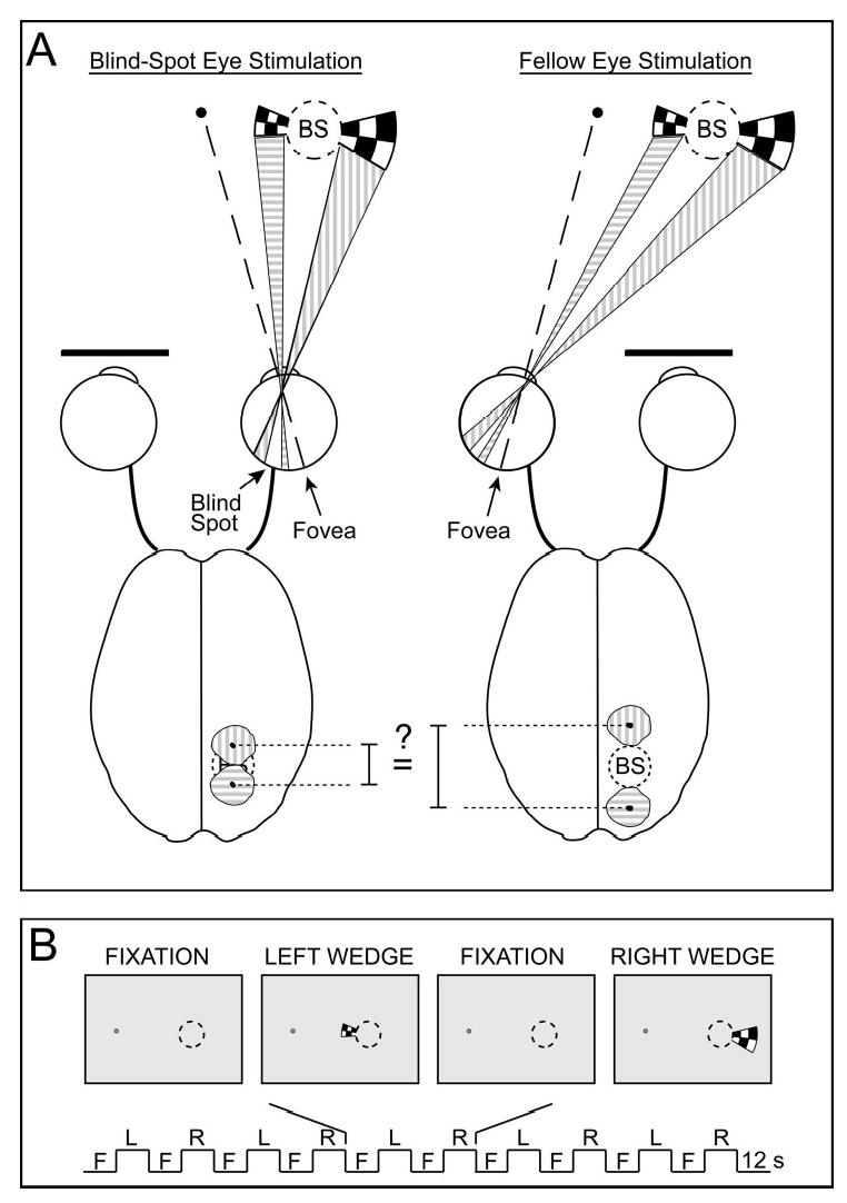
Experimental design and theoretical predictions of this study, shown in a schematic illustration. A: The passive remapping hypothesis predicts that independent stimuli presented to the left and right of the blind spot’s spatial location should lead to neighboring activations in visual cortex when the blind-spot eye is stimulated, but more separated activations when the fellow eye is stimulated. We tested this hypothesis by presenting wedges of flickering checkerboards independently to each eye, either to the left or to right of the blind spot’s spatial location. The wedges abutted the spatial location of the blind spot, and wedge sizes were adjusted to account for cortical magnification. B: During a single experimental run, wedges were alternately shown to the left (L) and to the right (R) of the blind-spot location for 12-s stimulus periods, interleaved between fixation rest periods (F).
METHODS
Observers
Four males, 27 – 33 years of age, participated in the study. Participants included two authors and two additional lab members who were naïve to the purpose of the study. All participants had normal visual acuity and were well experienced in fMRI experiments. All experiments were performed with the approval of Princeton University’s Institutional Review Panel for Human Subjects.
MRI Procedure
MRI scanning was performed with a head-only 3-Tesla Siemens Allegra scanner housed in the Department of Psychology at Princeton University using a standard birdcage head-coil. To minimize head motion, we used a custom bite-bar system to stabilize the participant’s head. The head stabilization reduced head motion to less than 1 mm throughout a session. A high-resolution anatomical scan was collected using a T1-weighted 3D MPRAGE sequence with 1-mm isotropic voxels. Functional BOLD signals were measured using gradient-echo echoplanar T2*-weighted imaging with the following parameters: TR 2000 ms, TE 40 ms, flip angle 90º, FOV 192 × 192 mm, matrix 64 × 64, in-plane resolution 3 × 3 mm, slice thickness 3 mm, 25 slices acquired perpendicular to the calcarine sulcus with no gap between slices.
Experimental Design and Stimuli
Visual stimuli were generated by a Macintosh computer, programmed in Matlab (The MathWorks Company) using the Psychophysics Toolbox software package (Brainard 1997). A luminance-calibrated Epson LCD projector was used to present stimuli on a rear-projection screen located beyond the subject’s head at the edge of the scanner bore. The screen had a diameter of 30 degrees when viewed through a mirror placed in front of the subject’s eyes. Subjects wore red-green anaglyph glasses, which allowed us to present luminance-calibrated stimuli to each eye independently (mean luminance through each filter, 7.4 cd/m2). In all experiments, the subject’s right eye served as the blind spot eye.
The study consisted of the following tasks: (1) behavioral localization of the blind spot’s spatial position, (2) fMRI localization of the blind spot’s cortical representation (2 runs), and (3) fMRI experiments to test for passive remapping of visual space around the blind spot (3-5 runs for each eye). The entire fMRI session lasted 2-2.5 hours. Experimental runs were about 4 min long, and required subjects to maintain steady fixation on a fixation point throughout the run. Retinotopic visual areas of each subject were identified in a separate MRI session using well-established methods (see Retinotopic mapping of visual areas). All MRI data collected in the blind-spot study were spatially aligned to each individual’s retinotopically defined visual areas.
(1) Localization of the blind spot’s spatial position
At the beginning of the MRI experiment, subjects first had to locate the position and extent of their right eye’s blind spot. Subjects were instructed to keep fixation on a bulls-eye (inner diameter 0.2º, outer diameter 1º) that was located 6º to the left of the screen’s center. A flickering disk was presented to the subject’s right eye, in a randomly selected position to the right of fixation. Using keys on a button box, subjects adjusted the size and position of the disk until it just vanished inside the blind spot. The size and position of the disk was recorded, and a new trial started with the appearance of the disk of another size and at an unpredictable position. Subjects performed a total of 3 blind-spot localization trials. Table 1 shows that subjects were able to map the spatial position and size of their blind spot reliably with standard deviations ranging from 0.01–0.31º. These reported positions and sizes are consistent with previous reports that the blind spot is somewhat variable across individuals, but is a vertically elongated ovoid region that roughly spans 4º × 6º, and positioned at about 15º eccentricity and about 2º below the horizontal meridian. The average size and position values of each subject’s blind spot were used to calculate the position and size of all subsequent visual stimuli.
Table 1.
Position and size of the blind spot for individual subjects
| Subject | Horizontal position (º) | Vertical position (SD) | Radius (SD) |
|---|---|---|---|
| S1 | 14.89 ± 0.01 | 0.04 (0.18) | 2.78 (0.07) |
| S2 | 16.76 ± 0.07 | −2.25 (0.05) | 2.78 (0.02) |
| S3 | 15.77 (0.07) | −0.95 (0.31) | 2.82 (0.09) |
| S4 | 15.77 (0.09) | −1.23 (0.24) | 2.92 (0.22) |
Mean and standard deviation of the blind spot’s size and position across 3 localization trials, shown in degrees of visual angle for individual subjects. These values were used to calculate the subsequent visual stimuli.
(2) Localization of the blind spot’s cortical representation
The cortical representation of the blind spot was identified using previously described methods (Tong and Engel 2001), by determining which cortical region responded more strongly to stimulation of the fellow eye as compared to stimulation of the blind-spot eye. A flickering checkerboard disk (size ~10º, contrast 80%, temp freq 7.5 Hz) that was twice the diameter of the right eye’s blind spot was alternately presented to the right blind-spot eye and to the left fellow eye. An fMRI run consisted of alternating 12-s periods of left-eye and right-eye stimulation, interleaved between 12-s periods of fixation rest. Subjects performed two fMRI runs for a total of 10 stimulus blocks for each eye. fMRI analyses consisted of multiple regression based on the general linear model, followed by linear contrasts, to identify brain regions that responded significantly more to stimulation of the left fellow eye than to stimulation of the right blind-spot eye. This contrast revealed selective activation of a small region in the fundus of primary visual cortex, anterior to the occipital pole, consistent with the known anatomical and functional location of the blind spot representation in human V1 (Tong and Engel 2001; Tootell et al. 1998).
(3) Testing for passive remapping at the blind spot
To test for passive remapping, we presented wedges of flickering checkerboards independently to each eye, either to the left or to the right of the blind spot’s spatial location (Fig.1A), and determined the corresponding regions of activation in early visual areas. The inner arcs of the wedge stimuli directly abutted the spatial location of the subject’s blind spot, which was drawn as a blank gray region. Although the stimuli were presented to only one side of the blind spot at a time during the fMRI experiments, we confirmed that simultaneous presentation of both stimuli on opposite sides of the blind spot led to perceptual filling-in for all subjects. The checkerboard wedges had a contrast of 80%, flickered at a rate of 7.5 Hz, and were adjusted in size to compensate for decreased cortical magnification in the periphery (Daniel and Whitteridge 1961) as illustrated in Figure 1. Actual wedge sizes were calculated based on the cortical magnification factor reported in a recent fMRI study (Duncan and Boynton 2003), and were adjusted so that each wedge had the same estimated horizontal extent in cortex as the blind spot itself. Therefore, wedge sizes varied slightly from subject to subject, with left wedges ranging from 3 – 3.4º and right wedges ranging 5.5 – 5.8º in the horizontal dimension.
In each fMRI run, stimuli were shown either to the right blind-spot eye or to the left fellow eye. The stimulus paradigm consisted of alternating 12-s periods of fixation rest and visual stimulation, with the flickering wedge shown to the left or to the right of the blind-spot location on alternate stimulus periods (Fig.1B). In each experimental run, the flickering wedge was presented 5 times on each side of the blind-spot location. Each subject performed 3-5 single experimental runs in which the stimuli were presented to the blind-spot eye, and an equal number of runs presented to the fellow eye.
Data analysis
All fMRI data underwent 3D motion correction using AIR (Woods et al. 1998), and subsequent analyses using BrainVoyager (Brain Innovation, Maastricht, The Netherlands). fMRI data underwent linear trend removal and were aligned to the high resolution, T1-weighted anatomical scan of the entire brain obtained in the same scan session. Talairach spatial normalization was applied to each subject’s brain to allow for reliable cortical segmentation and flattening (see Cortical segmentation and flattening procedures), and to transform the data into a common coordinate system. This ensured precise alignment of the MRI data for individual subjects across blind-spot mapping and retinotopic mapping sessions. The general linear model and multiple linear regression methods were used for all fMRI statistical analyses. Predictors for each stimulus condition (left wedge and right wedge) were set by convolving the relevant stimulus periods with a standard gamma function to account for the BOLD hemodynamic response. Separate activation maps for the left and right wedges were calculated for each fMRI run, which allowed us to compare the cortical locus of these activations across runs when either the blind-spot eye or the fellow eye was stimulated.
In each subject, we found separate cortical activations evoked by the left wedge and the right wedge in early visual areas. These activations were displayed on a cortical flat map of the subject’s brain, separately for each run. To ensure that a consistent and reliable criterion was used to localize cortical activations across different runs and conditions, the size of each cortical activation was held constant across runs by adjusting the statistical threshold to yield a region of interest of ~50 mm3 (see Fig. 3). This region corresponded well with the cortical volume that our wedge stimuli should have activated based on estimates of cortical magnification. We applied this criterion to all subjects, by matching the size of the cortical activations elicited by the left wedge and the right wedge on single runs, separately for area V1 and also V2/V3.
Figure 3.
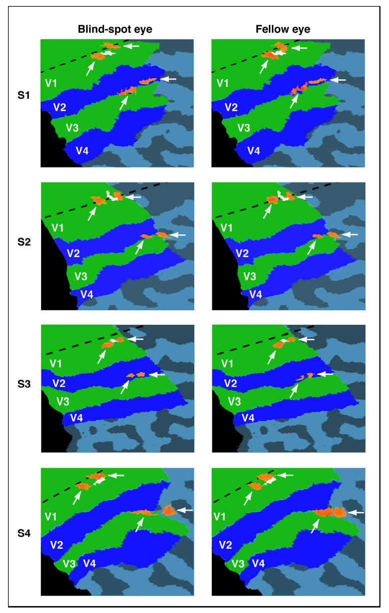
Cortical activation maps evoked by stimulation of the blind-spot eye (left column) and stimulation of the fellow eye (right column), shown on flat maps for all four subjects. Dashed lines indicate the horizontal meridian, and white regions near the horizontal meridian correspond to the V1 representation of the blind spot. Arrows point to activations evoked by the left and right wedges in early visual areas V1 and V2/V3. Statistical thresholds of these activations were adjusted separately to identify regions of peak activity of about 50 mm3 in volume (see Methods). Activations for each eye occurred in very similar locations of V1 and V2/V3, suggesting that the cortical representation of space around the blind spot is very similar for the two eyes.
To measure the cortical distance between activations corresponding to the left and right wedges on individual runs, we saved out the thresholded activation maps and performed subsequent analyses using Matlab (The MathWorks Company). We determined the centroids of the activations for the left wedge and the right wedge on the flattened representation of each subject’s Talaraich-normalized brain, and calculated the distance between the two centroids in a given area, e.g. V1. By separately analyzing individual fMRI runs for each eye, we were able to assess the reliability of cortical distance measures for each eye and to test for evidence of passive remapping (i.e., differences between the blind-spot eye and fellow eye).
Retinotopic mapping of visual areas
Retinotopic visual areas of each subject were identified in a separate MRI session using well-established methods (DeYoe et al. 1996; Engel et al. 1997; Sereno et al. 1995). Subjects maintained fixation while viewing ‘traveling wave’ stimuli consisting of rotating wedges and expanding rings, which were used to map cortical responses to changes in polar angle and eccentricity, respectively. Subjects were required to attend to the contrast-reversing checkerboard stimulus as it traversed the visual field by reporting whenever the stimulus briefly disappeared (for 53ms) at random intervals. Stimulus parameters were as follows: contrast 100%, temporal frequency 7.5 Hz, wedge size 45°, display radius 15°. The size of the wedge, ring, and checks were set to a fixed polar angle, and therefore increased in size as a function of eccentricity to compensate for cortical magnification (Daniel and Whitteridge 1961). Each fMRI run consisted of 10 cycles of mapping the visual field (32 sec/cycle), and subjects performed a total of 8 fMRI runs of polar angle mapping and 4 runs of eccentricity mapping.
Polar angle and eccentricity maps were created by calculating the average fMRI time series of each voxel, computing linear cross-correlation values with a predicted hemodynamic box-car function (duty cycle: 8s on, 24s off), determining the temporal phase that yielded the highest cross-correlation value for each voxel (threshold R ~0.25), and plotting the optimal phase values for polar angle and eccentricity tuning on a flattened representation of visual cortex. Boundaries between visual areas were delineated using field-sign mapping, which identifies reversals in the direction of polar angle phase encoding that run roughly orthogonal to the direction of eccentricity phase encoding (Sereno et al. 1995).
Cortical segmentation and flattening procedures
Cortical segmentation consisted of correcting for intensity inhomogeneities in the 3D anatomical image of each subject’s brain, applying Talairach spatial normalization, and using BrainVoyager’s auto segmentation region-growing algorithm to first identify boundaries between white and gray matter. The automatic gray-white matter delineation was visually inspected in detail, and fine-tuned corrections were performed manually. The resulting gray-white matter boundary map was used to create a 3-dimensional surface model of each subject’s brain. We “inflated” these surface models to obtain a smooth model of the brain where both sulci and gyri were visible on the surface. Virtual cuts were applied along the calcarine sulcus, and each subject’s surface model was then unfolded about the mid-brain, yielding a 2-dimensional “flat map” for each subject. The flattened representation involved minimal areal distortion of the 3D data (less than 14% on average). Retinotopic maps of visual areas were created using these flat maps.
In the present study, we constructed an alternative flat map that avoided cutting along the calcarine sulcus to ensure that the V1 representation of the blind spot remained intact. This involved applying virtual cuts along the lateral surface of the left hemisphere, including a cut along the lateral portion of the occipital lobe (roughly opposite to the calcarine sulcus), prior to cortical flattening. All cortical activations in this study were analyzed on these flat maps.
It should be noted that the average cortical distance measure obtained for each subject across all experimental conditions could reflect subtle spatial scaling effects due to Talairach transformation or slight variations due to cortical flattening. However, any such spatial scaling effects will remain constant across experimental conditions, and will not affect the interpretation of the results presented here, which emphasize the reliability of distance measures found within conditions and the reliability of any differences found across experimental conditions.
RESULTS
Localization of the blind spot’s cortical representation
We were able to localize the cortical representation of the blind spot in V1 by identifying the voxels that showed a greater response to stimulation of the fellow eye than to stimulation of the blind-spot eye. Figure 2 shows this activated region in a saggittal (A), coronal (B), and transverse (C) view of the brain, indicated as a white region highlighted by a surrounding red circle. The V1 representation of the right eye’s blind spot is located in the fundus of the calcarine sulcus in the left hemisphere. Figure 2 further shows an enlarged cutout of the flat map of the subject’s brain (D). The colored regions correspond to early visual areas V1, V2, V3, and V4 defined by retinotopic mapping (see Methods). The representation of the blind spot (white region) is located in the peripheral representation of V1 near the horizontal meridian, which runs through the middle of V1 roughly parallel to the V1/V2 boundary. Interestingly, the ‘hole’ resulting from the blind spot was only seen in area V1, and appeared filled-in at the level of V2.
Figure 2.
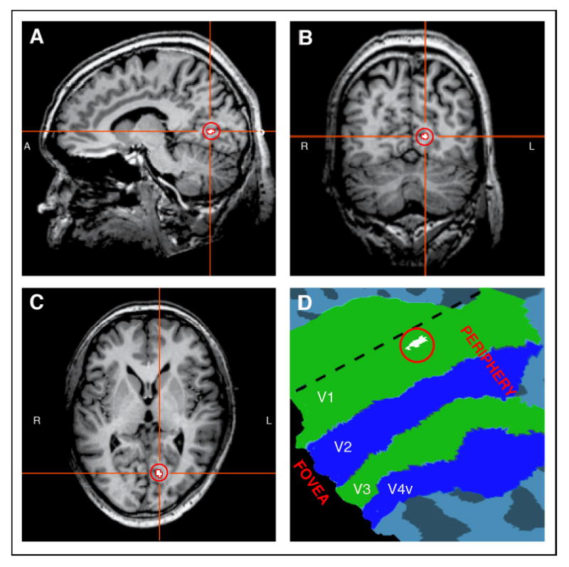
Cortical representation of the blind spot in V1, plotted in white and highlighted by a surrounding red circle, shown in sagittal (A), coronal (B), and transverse (C) views for a representative subject’s brain. This region responds more to stimulation of the fellow eye than to stimulation of the blind-spot eye. The V1 representation of the right eye’s blind spot is located in the fundus of the calcarine sulcus in the left hemisphere. D: V1 blind-spot region plotted on a flattened cortical map of retinotopic visual areas, V1- V4. The representation of the blind spot is located near the horizontal meridian (dashed line) in the periphery of V1.
Testing for passive remapping at the blind spot
To address the question of whether passive remapping occurs at the blind spot, we presented flickering checkerboard wedges separately to the left and to the right of the spatial location of the blind spot, and asked whether the cortical activations evoked by the wedges appear closer together when the blind-spot eye is stimulated than when the fellow eye is stimulated. Figure 3 shows the activation maps during stimulation of the blind-spot eye (left column) and fellow eye (right column) for all four subjects. Each subject shows separate activations (orange regions indicated by white arrows) corresponding to the left and right wedge in visual areas V1 and V2/V3, irrespective of whether we stimulated the blind-spot eye or the fellow eye. In area V1, activations are located near the horizontal meridian (dashed line) on opposite sides of the cortical representation of the blind spot (white region). Activations closer to the fovea correspond to presentations of the left wedge and the more peripheral activations correspond to presentations of the right wedge. The locations of, and the distance between, activations in area V1 are almost identical for the blind-spot eye and the fellow eye, suggesting that the representation of space in V1 is conserved for both eyes. Very similar results were found in area V2/V3, where activations appeared in the predicted location near the V2/V3 boundary corresponding to the horizontal meridian. Because the activations in area V2 closely bordered, and are not separable from, area V3, we will refer to these activations as being in area V2/V3. Again, activation maps appear to be qualitatively similar for the blind-spot eye and the fellow eye.
Next, we tested for passive remapping by quantifying the cortical distance between the centroid of each activation corresponding to the left wedge and the right wedge, when viewed by each eye (see Methods). According to the passive remapping hypothesis, cortical activations should appear closer together during stimulation of the blind-spot eye than during stimulation of the fellow eye. Figure 4A shows the cortical separation between activations in area V1 for all four subjects. The endpoints of each line depict the two centroids of activation, with line length indicating the cortical distance between activations corresponding to the left and right wedge. Thin grey lines show distance measures of single experimental runs and thick lines show mean distances across all runs for the blind-spot eye (solid) and fellow eye (dashed). For all subjects, we found almost identical activation positions and cortical distance measures for the blind-spot eye and the fellow eye. Figure 4B reveals that the magnitude of cortical distances were highly reliable and precise across single experimental runs, both for the blind-spot eye (black) and the fellow eye (white). The rightmost bars show the mean cortical distance and standard deviation across single experimental runs for each subject. The mean cortical distance, averaged across subjects, was 7.9 mm for the blind-spot eye and 7 mm for the fellow eye (Fig. 4B). The standard deviation across single experimental runs revealed an average error of less than 1 mm, indicating the high accuracy and reliability of our distance measures. The spatially precise measures found here are consistent with the high spatial precision of the fMRI BOLD signal as has been reported previously (Duncan and Boynton 2003; Engel et al. 1997). With these reliable cortical distance measures, we tested for evidence of passive remapping across the blind spot. A t-test, performed for each subject individually, revealed no statistically significant difference between cortical distance magnitudes during stimulation of the blind-spot eye and stimulation of the fellow eye for three out of four subjects (p = .22, .36, .50, respectively). One subject (S4) showed larger distance measures for the blind-spot eye than the fellow eye (t = 2.87, p < 0.05). Note however, that this difference runs contrary to the passive remapping hypothesis, which predicts that stimuli presented to the blind-spot eye should lead to neighboring or overlapping activations in cortex.
Figure 4.
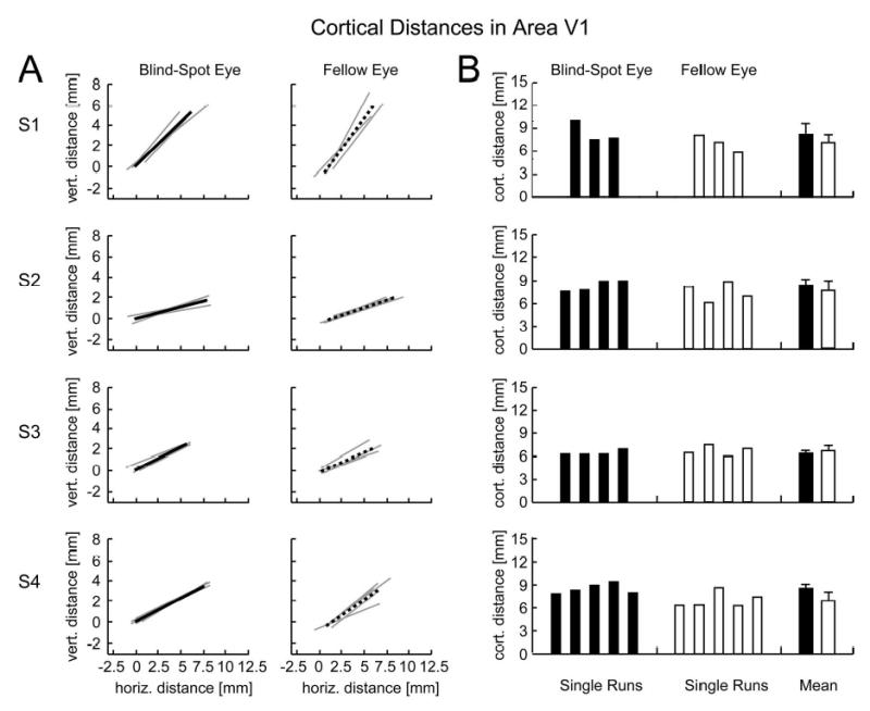
Cortical distances between activations in area V1 for all subjects. A: The endpoints of each line correspond to the centroids of activations for the blind-spot eye (left) and fellow eye (right), with line length indicating the cortical separation between activations to the left wedge and right wedge. Thin gray lines correspond to single experimental runs; thick lines show positions of peak activity after averaging across all experimental runs. All lines are plotted relative to the position of the centroid of mean activation evoked by the left wedge during stimulation of the blind-spot eye, with vertical and horizontal positions calculated relative to this anchor position for each flatmap image shown in Fig. 3. Activation positions and cortical distance measures are very similar for the blind-spot eye and fellow eye. B: Magnitude of cortical distances for single experimental runs and mean cortical distances across runs for the blind-spot eye (black bars) and fellow eye (white bars). Error bars, which represent standard deviations across single experimental runs, reveal an average error of 1 mm, indicating the high accuracy and reliability of our distance measures. Cortical distance measures for the blind-spot eye and fellow eye did not reliably differ in subjects 1-3. Subject 4 showed larger distance measures for the blind-spot eye than for the fellow eye, contrary to the predictions of the passive remapping hypothesis.
Figure 5 reveals very similar results in area V2/V3. All subjects showed only small variations across single fMRI runs. Mean cortical distances across subjects in area V2/V3 were 8.6 mm for the blind-spot eye and 6.9 mm for the fellow eye. Again, standard deviations were very small across experimental runs for individual subjects, with an overall average error value of 1.1 mm. Statistical analyses revealed no evidence of passive remapping in V2/V3. Three out of four subjects showed no statistically significant difference between cortical distance measures for the two eyes (p = .64, .37, .50 respectively). Subject 4 showed larger cortical distances for the blind-spot eye in V2/V3 as well (t = 6.12, p < 0.001), again contrary to the predictions of the passive remapping hypothesis.
Figure 5.
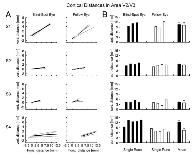
Cortical distances between activations in area V2/V3 (same conventions as in Figure 4). A: Line endpoints correspond to centroids of activations to the left and right wedges for the blind-spot eye (left) and the fellow eye (right). Thin lines, single fMRI runs; thick lines, average of all runs. B: Magnitude of cortical distances for single experimental runs and mean cortical distances across runs for the blind-spot eye (black bars) and fellow eye (white bars). Cortical distances for the blind-spot eye and fellow eye did not reliably differ for subjects 1-3. Subject 4 showed significantly larger distances for the blind-spot eye, contrary to the predictions of passive remapping.
Figure 6 shows a summary plot with the mean cortical distances for all subjects in both area V1 and area V2/V3. Mean cortical distance measures for each eye are superimposed to facilitate direct comparison between the blind-spot eye and the fellow eye. The similarity of the distance measures for the two eyes was further confirmed by additional within-subjects group analyses (t-test, p >.10), which revealed no statistical difference in cortical distance measures. If anything, there was a weak but non-significant trend for cortical distances to be larger for the blind-spot eye than for the fellow eye in area V1 and also in V2/V3, contrary to the predictions of the passive remapping hypothesis. We conducted additional t-tests to evaluate if a weak version of the passive remapping hypothesis might still be plausible. If one assumes that cortical distances for the blind-spot eye are at least 1 mm shorter than those for the fellow eye, then the likelihood of obtaining the results found here in V1 for each of the four subjects is p = .037, .029, .057, .00083 respectively. We can therefore reject the weak version of this remapping hypothesis for three out of four subjects, with the fourth subject (S3) showing a near-significant trend in the same direction. Similar results are obtained under these assumptions for area V2 (p = .14, .0083, .043, .00004 respectively). Therefore, it is highly unlikely that even modest effects of passive remapping, on the order of 1 mm, might account for these data.
Figure 6.
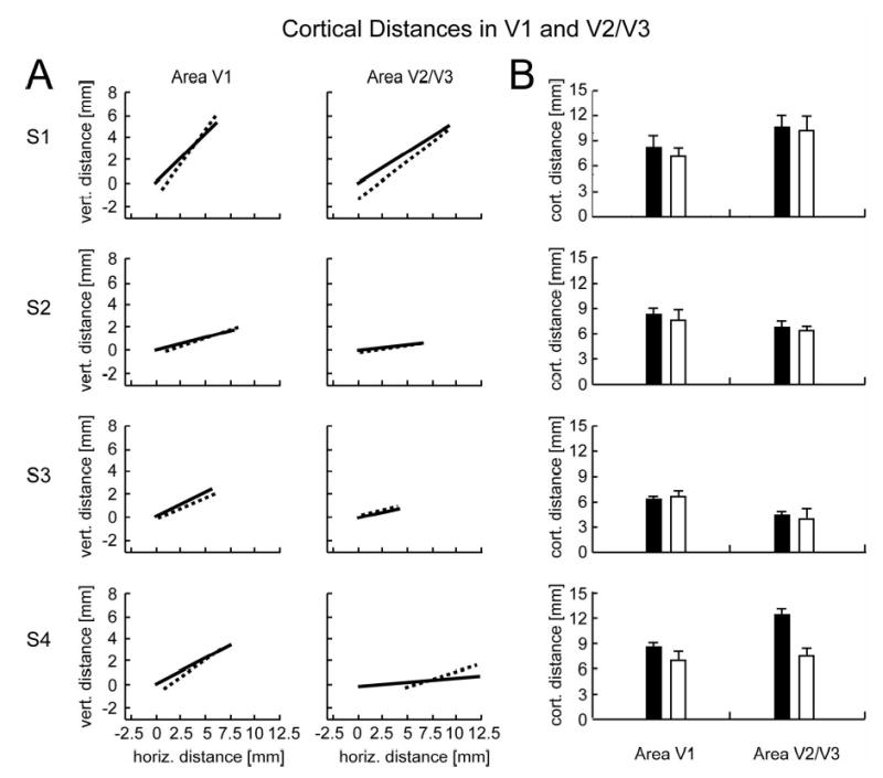
Direct comparison of mean cortical distances in areas V1 and V2/V3 for the blind-spot eye (solid lines/black bars) and fellow eye (dashed lines/white bars). A: Endpoints showing centroids of activations, averaged across all runs by subject, stimulus condition and visual area. B: Cortical distance magnitudes. Group analyses revealed no reliable overall difference in cortical distance measures for the two eyes.
The above results strongly suggest that the cortical distances between activation peaks for the blind-spot eye are virtually identical to those for the fellow eye, contrary to the predictions of passive remapping. However, it might be argued that passive remapping might still be taking place, not in terms of a shift in the location of peak activity but perhaps in terms of greater spread of activity into the blind-spot region. Even if activity peaks remain in the same position, the overall distribution of activity might still be skewed towards the blind-spot representation during stimulation of the blind-spot eye. We conducted additional analyses to test for any such skewing effects, by plotting the level of activation of each voxel along the cortex extending from the near side to the far side of the blind-spot representation. We observed the same pattern of results irrespective of whether t-values were used to estimate the signal-to-noise ratio of the response of each voxel or percent signal change was used to estimate the response amplitude of each voxel. Analysis results, based on t-values, are plotted in Figure 7.
Figure 7.
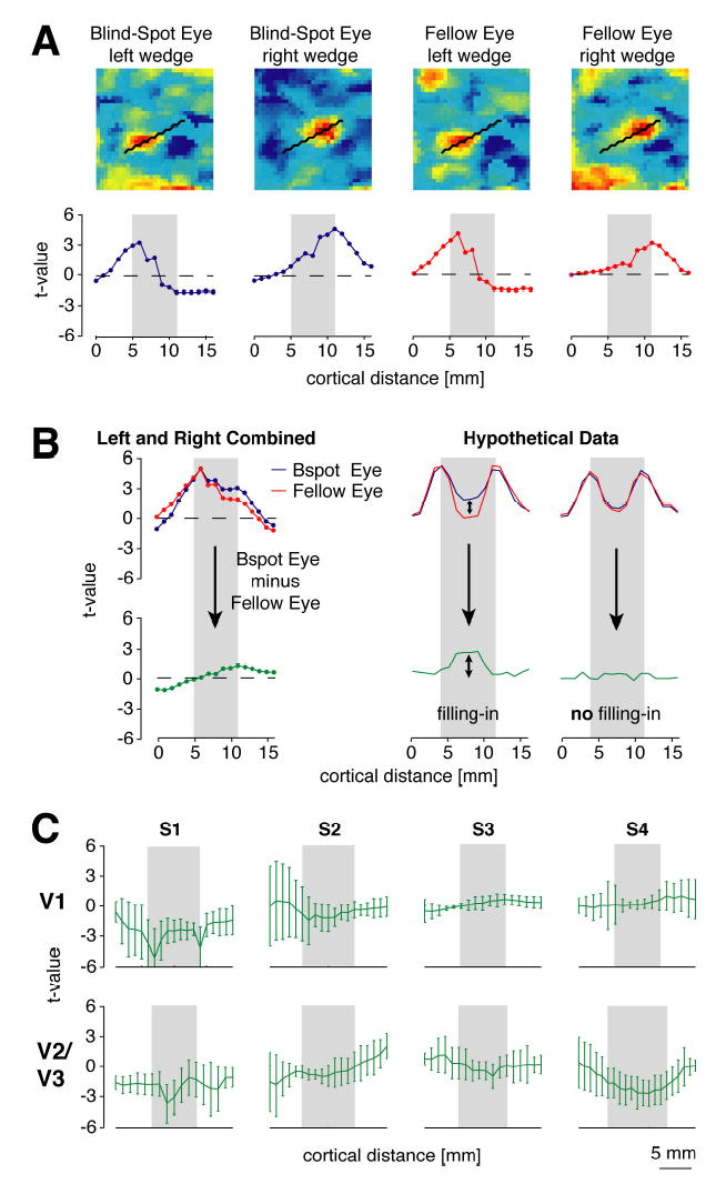
Spatial distribution of activity in V1 and V2/V3 during stimulation of the blind-spot eye (blue curves) and fellow eye (red curves). A: Above, example of V1 activation maps for left and right wedges presented to either eye of subject 3 on a single fMRI run (color coding: yellow-red, positive t-values; green-blue, negative t-values). Below, spatial distribution of activity across cortex for each stimulus condition on a single run. Activity levels were obtained from voxels positioned along a line connecting peak responses for all left wedge and right wedge runs (black line plotted on flatmaps). Within the two peaks of activity evoked by the left and right wedge (gray inset region) lies the cortical representation of the blind spot. T-values, which represent the signal-to-noise level of the response of each voxel, are plotted for all analyses. B: Sum of activity for left and right wedges, plotted by eye for two single runs of subject 3. Green curve shows the difference in summed activity for blind-spot eye (blue) minus fellow eye (red) conditions. If passive remapping occurs at the blind spot, then the resulting difference curve should be more positive in the cortical representation of the blind spot (which lies within the gray inset region) than outside of the blind-spot region (Figure 7B, hypothetical data). C: Difference curves (blind-spot eye minus fellow eye) for all four subjects in areas V1 and V2/V3. Error bars depict standard deviation of response differences across paired experimental runs. Contrary to the predictions of passive remapping, there was no evidence of greater activity in the blind-spot representation, relative to surrounding regions, in area V1 or V2/V3 of any subject.
Figure 7A shows examples of 2-D activation maps for individual runs of each stimulation condition, the 1-D line used to measure activity across cortex from one side of the blind-spot representation to the other, and the resulting 1-D spatial profile of activity. The left and right boundaries of the gray inset region correspond to the positions of peak activity evoked by the left and right wedges respectively. Within the gray inset region lies the cortical representation of the blind spot. To test if activity levels within the blind-spot representation proper might be elevated during stimulation of the blind-spot eye, we calculated the difference in activity for blind-spot eye minus fellow eye stimulation, based on the summed response of each eye to both wedge conditions (Fig. 7B). According to the predictions of passive remapping, difference maps should reveal elevated activity in the blind-spot representation (which lies within the gray inset region), relative to activity levels on either side of the blind-spot representation (Fig. 7B, hypothetical data). Our analyses revealed no evidence of spatial enhancement of activity in the blind-spot representation of V1 or V2/V3 for stimuli presented to the blind-spot eye, relative to the fellow eye (Fig. 7C). Therefore, analyses of both the spatial peaks of activity and the spatial distribution of activity revealed no evidence of passive remapping in these early visual areas.
DISCUSSION
In the present study, we investigated whether the blind spot is filled-in as a result of a remapping mechanism by which information from the blind spot’s surround is passively transferred into its cortical representation. Using fMRI, we measured the cortical distance between regions activated during stimulation on opposite sides of the spatial location of the blind spot to test if inputs from the blind-spot eye infiltrate the cortical representation of the blind spot. According to the passive remapping hypothesis, cortical distances should be much smaller for the blind-spot eye than for the fellow eye. Although the BOLD fMRI response is relatively blurred and can extend a few millimeters beyond the original site of neural activity (Engel et al. 1997), precise estimates of the spatial position and amplitude of these responses can be obtained by collecting many repeated measures (Duncan and Boynton 2003, Smirnakis et al. 2005). Our measures of cortical distance were highly precise and reliable, with standard deviations averaging only 1 mm across different experimental runs for individual subjects. With these spatially precise measures, we found virtually identical cortical distances for the blind-spot eye and the fellow eye in area V1 and also V2/V3. Moreover, stimulation of each eye led to very similar spatial distributions of activity, with no evidence of greater spreading of activity into the blind-spot representation during stimulation of the blind-spot eye.
Our results strongly suggest that the representation of space surrounding the blind spot is conserved for the two eyes such that stimuli presented to either eye, on either side of the blind spot’s spatial location, lead to activations in corresponding retinotopic locations in early visual areas. We found no evidence of passive remapping in areas V1 through V3 as determined by the sensitivity of our measures of BOLD activity, and were able to reject the likelihood of even very modest versions of the passive remapping hypothesis. Our results contrast fMRI studies of bilateral retinal lesions, which have revealed pronounced effects of cortical remapping in early human visual areas (Baker et al. 2005; Baseler et al. 2002). The lack of passive remapping found around the blind spot representation in the present study suggests that passive remapping in early visual areas is unlikely to account for all forms of perceptual filling-in.
Our fMRI results provide new evidence about the representation of space around the blind spot in human V1 that nicely complements previous neurophysiological studies in monkeys. Single-unit recordings from V1 neurons around the blind-spot representation suggest generally good agreement in receptive field maps for the two eyes (Komatsu et al. 2000; but see also Fiorani et al. 1992). Our measures of population activity using fMRI allowed for precise quantification of the degree of agreement in topographic maps for the two eyes, and indicate the neuronal filling-in responses in V1 are unlikely to reflect the effects of passive remapping. Instead, these responses are likely to reflect some contribution from active completion mechanisms (Fiorani et al. 1992; Matsumoto and Komatsu 2005), and perhaps also a general blurring of projections from retina to cortex that appear to be equally prevalent for both eyes.
The present study also provides novel evidence about the cortical representation of space around the blind spot in higher areas, namely areas V2 and V3. Due to the diffuse point-spread function of visual projections to area V4, it was not possible to precisely measure the central peaks of activity in this area. Nonetheless, the lack of any evidence of remapping in retinotopic areas V1 through V3 suggests that passive remapping is unlikely to have an important role in perceptual filling-in of the blind spot. Areas beyond V4, such as area MT or object-selective regions of human ventral temporal cortex, show even weaker retinotopic organization and would represent poor candidates for evaluating the effects of neuronal filling-in or passive remapping. The potential role of extrastriate visual areas in perceptual filling-in is further discussed below.
At which stage of the visual processing does filling-in occur?
Assuming that perceptual filling-in involves some type of active completion mechanism, the question arises as to whether this mechanism operates at an early or late stage of visual processing. Behavioral studies suggest that perceptual filling-in occurs at an early stage of visual processing. For instance, it has been shown that filling-in of the blind spot is driven by a sensory rather than a cognitive process that occurs automatically at a pre-attentive level (Ramachandran 1992b; Ramachandran and Gregory 1991). The perception of filled-in motion at the blind spot can lead to a motion aftereffect, indicating that filling-in can lead to the adaptation of direction-selective neurons (Murakami 1995). Perceptual filling-in can also enhance the dominance of a stimulus during binocular rivalry (He and Davis 2001). Given that binocular rivalry appears to be resolved in early visual cortices (Tong and Engel 2001), these findings suggest that filling-in of the blind spot begins to occur at an early stage of visual processing.
However, behavioral studies are not able to determine the precise stage at which filling-in occurs, and it remains unclear whether filling-in occurs at a single stage or across multiple stages of visual processing. One possibility is that perceptual filling-in arises from active completion in V1, and this filled-in information propagates to all higher visual areas. However, only a subpopulation of neurons in area V1 has shown evidence of active completion (Fiorani et al. 1992; Matsumoto and Komatsu 2005), and one might expect a much larger proportion of V1 neurons to show such effects if this region were solely responsible for perceptual filling-in. An alternative possibility is that filling-in occurs at multiple stages of visual processing, leading to greater neuronal filling-in of the blind spot in progressively higher visual areas.
In a recent study, Matsumoto and Komatsu (2005) suggested that filling-in of the blind spot may involve feedback signals from extrastriate areas to area V1. The authors based their hypothesis on the finding that average response latencies in V1 were about 12 ms slower for stimuli presented to the blind-spot eye as compared to the fellow eye. Longer latencies for the blind-spot eye did not seem to reflect the effects of slow conducting long-range horizontal connections because response latencies did not increase when more distal regions of a neuron’s receptive field were stimulated. Instead, the authors suggested that the longer latencies found for blind-spot eye stimulation may reflect the time required for feedforward signals to reach higher areas, such as V2, and then feedback to the V1 representation of the blind spot. Other evidence suggests that filling-in responses may be stronger in higher visual areas. For example, in the present study we were able to localize the V1 representation of the blind spot based on the fact that this region responds weakly to stimulation of the blind-spot eye and robustly to stimulation of the fellow eye. Interestingly however, no such differential activation was observed in higher visual areas, suggesting that filling-in responses may be stronger in V2 and higher areas. Single-unit studies of neuronal filling-in of artificial scotomas also implicate higher visual areas (De Weerd et al. 1995). An artificial scotoma refers to a blank peripheral patch that can be perceptually filled-in by dynamic surrounding texture after several seconds of steady fixation (Ramachandran and Gregory 1991). De Weerd and colleagues (1995) found that when a neuron’s classical receptive field lay well within an artificial scotoma, stimulation of surrounding regions with dynamic flickering texture could lead to gradual increases in neuronal activity over time. Interestingly, these neuronal filling-in responses to the artificial scotoma were most pronounced in area V3, somewhat evident in V2, but not evident in area V1. Although these findings strongly implicate higher visual areas in neuronal filling-in, an important distinction is that perceptual filling-in of artificial scotomas occurs gradually over several seconds whereas filling-in of the blind spot occurs instantaneously (Ramachandran and Gregory 1991). Important questions for future research include whether filling-in of the blind spot involves the same mechanisms as filling-in of the normal visual field, and whether visual areas beyond V1 are important for perceptual filling-in.
Conclusions
In the present study, we directly tested the passive remapping hypothesis of filling-in of the blind spot. We obtained highly reliable measures of cortical distances across the blind-spot representation, yet found no evidence of passive remapping in retinotopic visual areas V1 through V3. The representation of visual space around the blind spot was virtually identical for the two eyes, indicating that passive remapping is unlikely to account for neuronal filling-in of the blind spot in early visual areas. Instead, our results appear consistent with the predictions of the active completion theory. Future research will be important for revealing the precise neuronal mechanisms that mediate perceptual filling-in of the blind spot, and more generally, how the brain represents perceptual experiences in the absence of direct visual input.
Acknowledgments
The authors would like to thank D. Remus for technical assistance and the Center for Mind, Brain, and Behavior at Princeton University for MRI support.
Footnotes
GRANTS
This research was supported by grants from the National Institutes of Health (R01 EY14202) and the J. S. McDonnell Foundation to FT.
References
- Andrews PR, Campbell FW. Images at the blind spot. Nature. 1991;353:308. doi: 10.1038/353308a0. [DOI] [PubMed] [Google Scholar]
- Baker CI, Peli E, Knouf N, Kanwisher NG. Reorganization of visual processing in macular degeneration. J Neurosci. 2005;25:614–618. doi: 10.1523/JNEUROSCI.3476-04.2005. [DOI] [PMC free article] [PubMed] [Google Scholar]
- Baseler HA, Brewer AA, Sharpe LT, Morland AB, Jagle H, Wandell BA. Reorganization of human cortical maps caused by inherited photoreceptor abnormalities. Nat Neurosci. 2002;5:364–370. doi: 10.1038/nn817. [DOI] [PubMed] [Google Scholar]
- Brainard DH. The Psychophysics Toolbox. Spat Vis. 1997;10:433–436. [PubMed] [Google Scholar]
- Calford MB, Schmid LM, Rosa MG. Monocular focal retinal lesions induce short-term topographic plasticity in adult cat visual cortex. Proc R Soc Lond B Biol Sci. 1999;266:499–507. doi: 10.1098/rspb.1999.0665. [DOI] [PMC free article] [PubMed] [Google Scholar]
- Calford MB, Wang C, Taglianetti V, Waleszczyk WJ, Burke W, Dreher B. Plasticity in adult cat visual cortex (area 17) following circumscribed monocular lesions of all retinal layers. J Physiol 524 Pt. 2000;2:587–602. doi: 10.1111/j.1469-7793.2000.t01-1-00587.x. [DOI] [PMC free article] [PubMed] [Google Scholar]
- Chino Y, Smith EL, 3rd, Zhang B, Matsuura K, Mori T, Kaas JH. Recovery of binocular responses by cortical neurons after early monocular lesions. Nat Neurosci. 2001;4:689–690. doi: 10.1038/89469. [DOI] [PubMed] [Google Scholar]
- Daniel PM, Whitteridge D. The representation of the visual field on the cerebral cortex in monkeys. J Physiol (Paris) 1961;159:203–221. doi: 10.1113/jphysiol.1961.sp006803. [DOI] [PMC free article] [PubMed] [Google Scholar]
- De Weerd P, Gattass R, Desimone R, Ungerleider LG. Responses of cells in monkey visual cortex during perceptual filling-in of an artificial scotoma. Nature. 1995;377:731–734. doi: 10.1038/377731a0. [DOI] [PubMed] [Google Scholar]
- Dennett D Consciousness explained Boston, MA: Little Brown, 1991.
- DeYoe EA, Carman GJ, Bandettini P, Glickman S, Wieser J, Cox R, Miller D, Neitz J. Mapping striate and extrastriate visual areas in human cerebral cortex. Proc Natl Acad Sci U S A. 1996;93:2382–2386. doi: 10.1073/pnas.93.6.2382. [DOI] [PMC free article] [PubMed] [Google Scholar]
- Duncan RO, Boynton GM. Cortical magnification within human primary visual cortex correlates with acuity thresholds. Neuron. 2003;38:659–671. doi: 10.1016/s0896-6273(03)00265-4. [DOI] [PubMed] [Google Scholar]
- Durgin FH, Tripathy SP, Levi DM. On the filling in of the visual blind spot: some rules of thumb. Perception. 1995;24:827–840. doi: 10.1068/p240827. [DOI] [PubMed] [Google Scholar]
- Engel SA, Glover GH, Wandell BA. Retinotopic organization in human visual cortex and the spatial precision of functional MRI. Cereb Cortex. 1997;7:181–192. doi: 10.1093/cercor/7.2.181. [DOI] [PubMed] [Google Scholar]
- Fiorani M, Rosa MGP, Gattass R, Rocha-Miranda CE. Dynamic surrounds of receptive fields in primate striate cortex: A physiological basis of perceptual completion? Proc Natl Acad Sci USA. 1992;89:8547–8551. doi: 10.1073/pnas.89.18.8547. [DOI] [PMC free article] [PubMed] [Google Scholar]
- Gilbert CD, Wiesel TN. Receptive field dynamics in adult primary visual cortex. Nature. 1992;356:150–152. doi: 10.1038/356150a0. [DOI] [PubMed] [Google Scholar]
- He S, Davis WL. Filling-in at the natural blind spot contributes to binocular rivalry. Vision Res. 2001;41:835–840. doi: 10.1016/s0042-6989(00)00315-1. [DOI] [PubMed] [Google Scholar]
- Kaas JH, Krubitzer LA, Chino YM, Langston AL, Polley EH, Blair N. Reorganization of retinotopic cortical maps in adult mammals after lesions of the retina. Science. 1990;248:229–231. doi: 10.1126/science.2326637. [DOI] [PubMed] [Google Scholar]
- Komatsu H, Kinoshita M, Murakami I. Neural responses in the retinotopic representation of the blind spot in the macaque V1 to stimuli for perceptual filling-in. J Neurosci. 2000;20:9310–9319. doi: 10.1523/JNEUROSCI.20-24-09310.2000. [DOI] [PMC free article] [PubMed] [Google Scholar]
- Matsumoto M and Komatsu H Neural Responses in the Macaque V1 to Bar Stimuli with Various Length Presented on the Blind Spot. J Neurophysiol, 2005. [DOI] [PubMed]
- Murakami I. Motion aftereffect after monocular adaptation to filled-in motion at the blind spot. Vision Res. 1995;35:1041–1045. doi: 10.1016/0042-6989(94)00201-v. [DOI] [PubMed] [Google Scholar]
- Murakami I, Komatsu H, Kinoshita M. Perceptual filling-in at the scotoma following a monocular retinal lesion in the monkey. Vis Neurosci. 1997;14:89–101. doi: 10.1017/s0952523800008798. [DOI] [PubMed] [Google Scholar]
- Pessoa L, Thompson E, Noe A. Finding out about filling-in: a guide to perceptual completion for visual science and the philosophy of perception. Behav Brain Sci. 1998;21:723–748. doi: 10.1017/s0140525x98001757. discussion 748–802. [DOI] [PubMed] [Google Scholar]
- Ramachandran VS. Blind spots. Sci Am. 1992a;266:86–91. doi: 10.1038/scientificamerican0592-86. [DOI] [PubMed] [Google Scholar]
- Ramachandran VS. Filling in the blind spot. Nature. 1992b;356:115. doi: 10.1038/356115a0. [DOI] [PubMed] [Google Scholar]
- Ramachandran VS, Gregory RL. Perceptual filling in of artificially induced scotomas in human vision. Nature. 1991;350:699–702. doi: 10.1038/350699a0. [DOI] [PubMed] [Google Scholar]
- Schmid LM, Rosa MG, Calford MB, Ambler JS. Visuotopic reorganization in the primary visual cortex of adult cats following monocular and binocular retinal lesions. Cereb Cortex. 1996;6:388–405. doi: 10.1093/cercor/6.3.388. [DOI] [PubMed] [Google Scholar]
- Sereno MI, Dale AM, Reppas JB, Kwong KK, Belliveau JW, Brady TJ, Rosen BR, Tootell RB. Borders of multiple visual areas in humans revealed by functional magnetic resonance imaging. Science. 1995;268:889–893. doi: 10.1126/science.7754376. [DOI] [PubMed] [Google Scholar]
- Smirnakis SM, Brewer AA, Schmid MC, Tolias AS, Schuz A, Augath M, Inhoffen W, Wandell BA, Logothetis NK. Lack of long-term cortical reorganization after macaque retinal lesions. Nature. 2005;435:300–307. doi: 10.1038/nature03495. [DOI] [PubMed] [Google Scholar]
- Tong F, Engel SA. Interocular rivalry revealed in the human cortical blind-spot representation. Nature. 2001;411:195–199. doi: 10.1038/35075583. [DOI] [PubMed] [Google Scholar]
- Tootell RB, Hadjikhani NK, Vanduffel W, Liu AK, Mendola JD, Sereno MI, Dale AM. Functional analysis of primary visual cortex (V1) in humans. Proc Natl Acad Sci U S A. 1998;95:811–817. doi: 10.1073/pnas.95.3.811. [DOI] [PMC free article] [PubMed] [Google Scholar]
- Tripathy SP, Levi DM, Ogmen H. Two-dot alignment across the physiological blind spot. Vision Res. 1996;36:1585–1596. doi: 10.1016/0042-6989(95)02200-7. [DOI] [PubMed] [Google Scholar]
- Walls GL. The filling-in process. Am J Optom Arch Am Acad Optom. 1954;31:329–341. doi: 10.1097/00006324-195407000-00001. [DOI] [PubMed] [Google Scholar]
- Woods RP, Grafton ST, Holmes CJ, Cherry SR, Mazziotta JC. Automated image registration: I. General methods and intrasubject, intramodality validation. J Comput Assist Tomogr. 1998;22:139–152. doi: 10.1097/00004728-199801000-00027. [DOI] [PubMed] [Google Scholar]