

Abstract
We have developed a microfluidic mixer for studying protein folding and other reactions with a mixing time of 8 μs and sample consumption of femtomoles. This device enables us to access conformational changes under conditions far from equilibrium and at previously inaccessible time scales. In this paper, we discuss the design and optimization of the mixer using modeling of convective diffusion phenomena and a characterization of the mixer performance using microparticle image velocimetry, dye quenching, and Förster resonance energy-transfer (FRET) measurements of single-stranded DNA. We also demonstrate the feasibility of measuring fast protein folding kinetics using FRET with acyl-CoA binding protein.
In protein folding, important structural events occur on a microsecond time scale.1 To study their kinetics, folding reactions must be initiated at even shorter time scales. Photochemical initiation2 and changes in temperature,3 pressure,4,5 or chemical potential, as in salt or chemical denaturant concentration changes,6–9 all provide the perturbation of protein conformational equilibria necessary to initiate folding. Laser temperature-jump relaxation provides the best temporal resolution with dead times in the nanosecond range,3 but only a small number of proteins denature reversibly at elevated temperature. Temperature-jump techniques are also limited to conditions near the equilibrium unfolding transition where marginally stable folding intermediates are less likely to accumulate. Pressure relaxation initiates the folding process by exploiting a change in the volume between the folded and unfolded conformers. Pressure changes up to 20 MPa in under 100 μs have been created with piezoelectric devices to monitor rate-limiting barrier crossing in the cold shock protein with Förster resonance energy transfer (FRET).10 However, in pressure-jump experiments, the folding equilibrium is shifted only marginally at low denaturant concentrations where collapse occurs, and chain collapse is therefore not easily measured via FRET as refolding amplitudes are small.10–12
In comparison to temperature- and pressure-jump relaxation techniques, folding experiments based on changes in chemical potential, via rapid mixing of protein solutions in to and out of chaotrope solvents, are more versatile. The technique is applicable to a wide range of proteins as most unfold reversibly in the presence of chemical denaturants such as urea7 and guanidine hydrochloride (GdCl).6 Further, mixer-based experiments are not limited to proteins near the folding transition state. Until recently, the main limitation of mixer-based experiments was their inability to access very short time scales. Mixing of chemical species is ultimately limited by the time required for molecular diffusion across a finite length scale and diffusion time scales as the square of diffusion length.13,14 Diffusion lengths can be reduced greatly with turbulent fluid motion, but this requires high flow rates to achieve high Reynolds numbers.15 The fastest commercially available stop-flow mixing devices use turbulent flow and have dead times of ~0.25 ms (e.g., see BioLogic, Claix, France). Custom-designed turbulent mixers have been used to study protein folding with circular dichroism16 and small-angle X-ray scattering (SAXS)17 with dead times on the order of a few hundreds of microseconds and sample mass consumption as high as 8 mg/s. The shortest reported mixing times of ~50 μs in turbulent devices were demonstrated by a continuous-flow mixer but with sample consumption of up to 0.6 mL/s.9 The high sample consumption of turbulent mixers limits their applicability, as many proteins are difficult or expensive to prepare. Finally, there is typically no or inadequate optical access to the mixing process in stopped-flow and continuous-flow turbulent mixers, resulting in a dead time during which the reaction cannot be observed.
Brody et al.13 first proposed rapid mixers based on hydrodynamic focusing as a way to address the issue of reducing diffusion lengths under laminar flow conditions while minimizing sample consumption. Hydrodynamic focusing has been used in combination with SAXS17,18 and FT-IR spectroscopy19 to measure protein and RNA folding,20 with mixing times of a few hundreds of microseconds. Pabit and Hagen21 also demonstrated a laminar flow device that allowed UV excitation and emission.
Our mixer is based on a continuous-flow device by Knight et al.,22 which leverages hydrodynamic focusing23 on the micrometer scale to reduce diffusion lengths. This mixing method uses hydrodynamic focusing to form a submicrometer liquid stream of denatured protein solution. As denaturant diffuses away from the stream, individual proteins experience a decreasing local denaturant concentration and start to refold. This mixing process can be qualitatively divided into two phases. First, the incoming stream of denatured proteins is focused into a thin sheet, and second, the denaturant diffuses out of this thin stream with a diffusive flux largely oriented in a direction normal to liquid flow streamlines. Since residence time in the upstream focusing region is significant, molecular diffusion during both of these phases has to be considered.
This paper discusses the design, optimization, and characterization of our microfluidic mixers. These mixers use over 8 orders of magnitude less labeled protein sample mass flow than a previously reported ultrafast protein folding mixer,9 with flow rates of 3 nL/s and protein concentrations of tens of nanomolars. We propose a quantitative definition of mixing time appropriate for this application and quantify the mixing performance of our mixer using both dye-quenching measurements and fluorescence measurements of FRET-labeled DNA. We show the feasibility of studying protein folding using acyl-coA binding protein as a model system and demonstrate the accessibility of both submicrosecond and -millisecond time scales. Although this work is focused on protein folding experiments, the mixer device presented here may also be useful in the study of other nonequilibrium biophysical and biochemical processes that require fast mixing and high rate-of-strain fields (e.g., polymer dynamics24 and enzymatic reactions25).
THEORY AND MODELING
Convective Diffusion Mixing of Protein Streams
The mixer flow was analyzed using numerical solutions of the full Navier–Stokes fluid flow equations and a convective diffusion equation describing concentration fields of the denaturant GdCl. These flow simulations were used to explore the performance of a variety of mixer designs with systematically varied flow and geometric parameters. We used a commercially available, open-source code (FEMLAB by Comsol Inc., Stockholm, Sweden) for solutions of steady Eulerian-frame velocity and concentration fields. The model is applied to mixer designs with the general three-inlet/single-outlet channel architecture proposed by Knight et al.22 The basic design consists of a sample stream that enters the mixing region through a center nozzle of width wc, focused by two symmetric side channels with a characteristic width ws. We approximate flow at the vertical midplane with two-dimensional (2D) flow simulations,26 as the channel depth of our design is greater than five to six times the nozzle width. The nondimensionalized Navier–Stokes equations of motion are given by
| (1) |
The scaling is as follows: α = wc/ws, γ = we/wc, β = Us/Uc, and a Reynolds number defined as Rew = Usws/v, where U is the maximum velocity, w is the sample nozzle width, and v is the kinematic viscosity of the solution. u and v are scaled using Uc and Us, respectively, and pressure is scaled as Ucμ/wc, where μ is the dynamic viscosity. The subscripts s, c, and e refer to the side, center, and exit channels. Note that the full Navier–Stokes formulation is appropriate as Rew values were as high as 15. At steady-state conditions, conservation of a species i can be expressed as
| (2) |
where PeDi = Ucwc/Di is the Peclet number27 based on nozzle width. We use a simple Fick diffusion27 as scaling approximations and simple one-dimensional models show that liquid junction potentials28 are negligible. We are interested in the convective diffusion of the protein denaturant GdCl, i = g, and the sample protein, i = p. The steady, 2D velocity field and concentration fields of the model are approximately characterized using the five nondimensional parameters: α, β, γ, Rew, and PeD. Equations 1 and 2 are subject to the following boundary conditions:
| (3) |
| (4) |
where denotes the location of walls and is the wall unit normal vector. Equation 3 accounts for no-slip and no-penetration boundary conditions, and eq 4 enforces the condition of zero diffusional flux at the walls. For the velocity and length scales of interest, PeDp is ~100 times larger than PeDg, so the right-hand side of eq 2 is negligible for protein species. That is, proteins will approximately follow streamlines of the flow.
A number of physical limitations of the problem impose constraints on the optimization. The lithography step in fabrication limits the minimum feature size to 1–2 μm. We also limited the width of the side channel nozzles, ws, to 3 μm to mitigate clogging issues. Contaminants left over from the fabrication process and present in the buffers would often clog the side channels at the nozzle. Clogging was kept to a minimum with filter post spacings of 1–2 μm and side nozzle widths of 3 μm. We constrained the depth of the channels to ~10 μm to optimize the fluorescence signal with a confocal system and because we intend to build future devices out of fused silica, which is difficult to etch deeper. The physical properties of buffers and denaturants commonly used for protein folding studies have known parameters such as density, viscosity, and diffusivity. Our models were 2D approximations to the physical system; thus, we constrained the maximum aspect ratio (aspect ratio = width/depth) of the regions of interest to less than unity. This aspect ratio constraint ensures approximately 2D fluid flow at the vertical midplane of the mixer. To summarize these physical limitations: (1) Minimum feature size due to lithography was 1 μm; (2) minimum side channel nozzle widths were 3 μm to mitigate clogging; (3) maximum channel depth was 10 μm due to imaging and future fabrication limitations; (4) common denaturant and buffer solutions fixed values for density, viscosity, and diffusivity; and (5) 2D model assumptions limited the maximum aspect ratio to unity.
Together constraints 1, 3, and 5 above set a maximum γ of γmax = 10. We know from fluorescence imaging experiments that the flow in the nozzle region becomes highly three-dimensional for Rew greater than ~20, even for center channel width-to-depth ratios of less than 0.2. We therefore imposed a maximum working condition of Rew,max = 15, which, together with the constraints on channel geometry, sets a maximum flow rate of ~200 nL/s for the two inlet side channels.
Definition of Mixing Time
There are no general definitions of mixing time, and several definitions of the degree of mixing exist in the literature.29–31 In most cases, the best definition of mixing time is an ad hoc rule that takes into account the figures of merit of a specific application. We here propose a mixing definition for our mixer that well characterizes the temporal resolution of subsequent macromolecular folding kinetics measurements. We define mixing time as the time required to change the local denaturant concentration in the region around a typical protein molecule from 90 to 10% of the initial value (10% is well below the concentration required to initiate folding for most proteins). This mixing time is based on the unsteady Lagrangian denaturant concentration experienced by a single protein as it flows through the center (y = 0) streamline of the mixer. The unsteady Lagrangian concentration can be obtained by time-integrating the (steady) Eulerian velocity fields along the center streamline. The Lagrangian denaturant concentration of a protein flowing along a streamline is then
| (5) |
where
| (6) |
and u and v are the x- and y-coordinate components of the Eulerian velocity field evaluated at the coordinates of the protein (xp,yp). cgL and cg are the Lagrangian and Eulerian concentration variables, respectively. Note that cg(x,y) is the steady scalar concentration field of denaturant, while cgL is an unsteady, local denaturant concentration which has time, t, as a unique independent parameter. The Eulerian velocity field, (u,v), is obtained from solutions to eq 1.32 The Lagrangian concentration history for a protein flowing along the symmetry line is described by evaluating cgL for ū(y = 0).
We compared various mixer geometries and flow conditions in order to optimize mixer performance. To this end, we used the following mixing time, tmix, as a cost function in the optimization:
| (7) |
where
| (8) |
where y10 and y90 are respectively the locations along the line of symmetry where the denaturant concentration is locally 10 and 90% of the initial concentration value, cgo.
Design and Optimization
We optimized the shape and conditions for our mixer designs using the model described above. In evaluating mixing time for a given design, we adhered to the following procedure. We first proposed a geometry with the basic cross-shape architecture and a specific combination of the parameters α, β, γ, Rew, and PeD. These designs were subject to the constraints described above. Second, we performed Eulerian field simulations using eqs 1–4. Third, we applied eqs 5–8 to evaluate Lagrangian concentration fields and mixing time. This third step constitutes a full iteration of the design procedure. In subsequent iterations, we vary one or more of the five mixer parameters and then repeat the process to minimize the cost function, tmix.
MATERIALS AND DEVICE FABRICATION
The geometry suggested by our optimization was fabricated (13 devices/wafer) on silicon substrates using contact photolithography (with electron beam masks), deep reactive ion etching, and anodic bonding of a 170-μm-thick Pyrex 7740 wafer (Sensor-Prep Services) to seal the channels. This fabrication method limits the minimum feature size to one to two microns. Figure 1a shows a reflection optical image of the mixer. The lengths and widths of the supply channels leading to the nozzle region were chosen to produce pressure drops on the order of 1 MPa and thereby reduce the effects of pressure control fluctuations. The sample supply channel was 10 μm wide and 27 mm long. Side channel supply channels were typically 60 μm wide and 9 mm long. These dimensions were chosen to provide total pressure drops on the order of 700 kPa at the flow rates of interest. This resulted in steady flow conditions that were robust to the order of 0.7 kPa fluctuations of the pressure control system. Figure 1b shows the mask image of the entire chip used in the fabrication process. All channels were etched to a depth of 10 μm. The designs use integrated filters (visible in Figure 1a as three large black regions near the nozzles) to reduce clogging of the nozzles. The filters consist of an array of 2-μm-diameter posts arranged so that the clearance space between posts decreased from 4 μm to as small as 1 μm in the flow direction as shown in Figure 1c. We found clogging was kept to a minimum with filter spacing of 1–2 μm and side channel widths of 3 μm. Figure 1d shows an isometric SEM image of an optimized nozzle and mixer region. The shape of the transition regions between the supply channels and the mixer inlet nozzles was chosen simply by limiting the convergence angle of the passageways to less than 45°. We also incorporated simple circular arcs of 1-μm radii for corners in the model, consistent with the limits of the photolithography.
Figure 1.
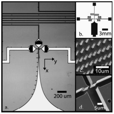
Images of silicon microfluidic mixer. (a) CCD image of mixing region showing three inlet channels with integrated filters (center and side channels), nozzle region at intersection, and exponential mixer exit region (south channel). Dots along the mixing channel are distance markers. (b) Schematic (mask) of the entire microfluidic chip. The inlet (center and side) and exit channels were sized (length and width) to reduce instabilities of focused stream from pressure controller fluctuations. (c) SEM image of filter posts in inlet channels upstream of nozzle region. The filters consist of rows of 1–2-μm spaced posts to avoid clogging. (d) SEM images of nozzles and initial mixing region. Nozzle widths are ~1–3 μm wide and channels are 10 μm deep.
We designed the exit channel to have a 200-μm-long, constant-width section where fully developed flow provides a uniform centerline velocity. In this region, the Eulerian centerline coordinate of a protein is a linear function of time. Beyond this section, two mixer designs were fabricated where the exit width increases either linearly or exponentially, as shown in the bottom of Figure 1a. The exponential expansion reduces the outlet stream centerline velocity exponentially, so that the Eulerian centerline coordinate of a protein scales as the logarithm of time. Using the exponential design, we can resolve time scales from less than 10 μs to hundreds of milliseconds in a single experiment. Our mixers typically operate for 20–100 h of run time (useful for more than several days of experiments) before clogging, require as little as 10–20 μL of loaded sample volume, and consume ~3 nL/s of sample. Initial designs we tested without integrated filtering have typical maximum run times of just a few hours.
The microchips are coupled to an acrylic or Teflon reservoir and pressurized using two computer-controlled pressure regulators with a 0–150 psi pressure range and 0.1% accuracy (Marsh Bellofram Inc.). The two regulators allow precise independent control of flow rates in the center and two side inlet channels. The interconnect fixture also facilitates changing of sample solutions without removing the device from the microscope. We performed SEM visualization on one mixer for each wafer to characterize the 3D geometry. Mixers within each batch varied slightly in channel and nozzle widths, with typical variations of less than 10%. We imaged each mixer after use with wide-field, reflective-mode microscopy with 40× and 60× magnification lenses (NA ranging from 0.6 to 0.7) to quantitate the geometry used for simulations.
A poly(ethylene glycol) (PEG)-derived polymer solution was used to reduce adsorption of molecules onto the walls of the mixer.33–36 The copolymer poly(l-lysine)-g-poly(ethylene glycol) (PLL-g-PEG) was dissolved in deionized water (DI) at 1 mg/mL and flushed through all channels of the mixer prior to quenching, DNA, and protein experiments. We then flushed filtered DI through the mixer to remove the polymer solution leaving just the channel walls coated with the polymer.
FLOW AND REACTION DIAGNOSTICS
Microparticle Image Velocimetry (Micro-PIV)
Flow profiles and pressure–velocity calibrations were measured using cross-correlation micro-PIV using the method and instruments described by Santiago et al.37 and Devesenathipathy et al.38 The mixers were filled with a suspension of 200-nm polystyrene beads doped with fluorescent dye (Molecular Probes). The fluorescent particles were illuminated with a dual-head, frequency-tripled Nd:Yag laser with a pulse width of 7 ns and times between pulses as low as 700 ns. Images of the flow were obtained using a Nikon plan achromat oil immersion, 1.4 NA, 60× objective mounted on a TE300 inverted epifluorescent microscope (Nikon) and recorded using a cooled interline transfer CCD camera (Princeton Instruments). Image data was analyzed with a PIV code developed by Wereley.39
Dye Quenching
Typical mixer characterization techniques for determination of mixing times use quenching of the fluorescence of a slowly diffusing dye mixed with a buffer containing a fast-diffusing quencher.40,41 This method decouples the dynamics associated with the diffusion of the dye from those of the quencher. We effectively measured the diffusion of the iodide ions into the focused dye stream by quenching a large molecular weight fluorescent dye with potassium iodide. The decrease in quantum yield of the dye molecules is due to collisional quenching, which opens a nonradiative relaxation path for the excited electron. The decrease in fluorescence intensity is proportional to the local concentration of iodide ions42 and can be used to directly measure salt concentration. The change in fluorescence is characterized with the unquenched-to-quenched intensity ratio. We quenched 2 MDa dextran-conjugated fluorescein (Molecular Probes) at 10 μM with a solution of 500 mM KI. Both solutions were prepared in 10 mM phosphate-buffered saline (pH 7.4). The quenching data are then compared to an unquenched case where the dye is mixed with pure buffer without KI.
Single-Stranded DNA (ssDNA) Synthesis, Labeling, and Characterization
DNA oligonucleotides (dT)30 were prepared by automated total synthesis using a DNA/RNA synthesizer (model 392, Applied Biosystems) using commercial reagents (Glen Research Corp.). We used high-pressure liquid chromatography-purified trityl-ON DNA fragments using a C2/C18 μRPC column on an ÄKTA FPLC device (Amersham Pharmacia Biotech). The fragments were labeled with amine-reactive TMR and Alexa 647 (Molecular Probes). Further purification removed unattached dye molecules. Samples were kept at −20 °C and diluted in single-molecule buffer before use.43 We filtered all buffers before use with 0.1-μm-pore diameter filters.
Single-molecule nanosecond alternate laser excitation measurements were performed as described by Laurence et al.44 to determine proximity ratios between the two fluorophores for various salt concentrations (excluding signal from donor- or acceptor-only molecules). This technique also determined the amount of donor-only (<5%) and acceptor-only (not detected) labeled molecules in the sample.
Protein Expression, Purification, and Labeling
A double-Cys variant (Ser2Cys/Ile86Cys) of acyl-CoA binding protein (ACBP) was expressed in Escherichia coli BL21 and purified as described by Teilum et al.45 For labeling of ACBP with a single-dye FRET pair, we reacted a quantity of pure ACBP in 20 mM sodium phosphate (pH 7.0, 100 mM sodium chloride) with Alexa 488 (FRET-donor) at 1:1 stoichiometry and incubated for 4 h at ambient temperature in the dark. After buffer exchange into 10 mM Tris (pH 8.0), we separated single-labeled Alexa 488–ACBP from double-labeled and nonlabeled ACBP with MonoQ anion-exchange chromatography (Amersham Pharmacia). Elution of resin-bound protein was achieved using a sodium chloride salt gradient. We then concentrated the fraction containing single-labeled Alexa 488–ABCP and buffer-exchanged into 20 mM sodium phosphate (pH 7.0). The protein solution was reacted with a 10-fold stoichiometric excess of Alexa 647 (FRET-acceptor) for 4 h at ambient temperature in the dark. We separated double-labeled Alexa 488/Alexa 647–ACBP from side products using MonoQ anion-exchange chromatography and stored at 4 °C in the dark until use. Matrix-assisted laser desorption/ionization time-of-flight mass spectrometry guaranteed homogeneity of the final product.
For protein refolding experiments, we denatured the double-labeled Alexa 488/Alexa 647–ACBP for 2 h in 6 M GdCl in 20 mM sodium acetate (pH 5.3, 0.001% bovine serum albumin (BSA)) at a concentration of 80 nM. Single-molecule FRET experiments on diffusing molecules indicate quantitative unfolding of ACBP under these conditions, as supported by a disappearance of the high FRET native subpopulation (with a Förster energy-transfer efficiency of E = 0.9) and the simultaneous appearance of a broader distribution of denatured molecules with E centered around 0.3 (unpublished data). We initiated the refolding reaction in the mixer using 20 mM sodium acetate (pH 5.3, 0.001% BSA).
Confocal Microscopy and Image Analysis
Fluorescence images were acquired using a stage-scanning confocal microscope controlled by custom software developed in LabView (National Instruments), similar to that described by Lacoste et al.46 The confocal setup is based on an IX71 inverted microscope (Olympus) with an oil immersion, 1.4 NA, 60× objective, a 35- or 50-μm pinhole, and a nanometer-resolution three-axis piezostage (Nano-LP200, MadCity Labs). The fluorescent dyes were excited using a multiline argon ion laser (ILT 5490A, Midwest Laser), and we detected donor and acceptor signals with avalanche photodiodes (SPCM-AQR-14, Perkin-Elmer Optoelectronics, Quebec, CA). A counting board (PXI-6602, National Instruments) provided 12.5-ns resolution of arrival time for each detected photon. We reconstructed color-coded images by binning photons according to the pixel scan duration. Emission filters (EF, Omega Optical) and dichroic mirrors (DM, Chroma Technology Corp) depended on the donor/acceptor pair used.47 Typical scans were 90 μm (X) × 4 μm (Y), with 0.25–1 μm streamwise resolution and a 0.1-μm transverse resolution. The integration per pixel was adapted to obtain a sufficient signal-to-noise ratio and varied between 5 and 50 ms, with excitation intensity at the objective back focal plane of 25–200 μW. Proximity ratio profiles, after background subtraction, were obtained along the focused stream using geometrical weighting of each image pixel. For the ssDNA collapse experiment, we calculated the conversion of proximity ratio data into salt concentration data in two steps. For each new optical alignment, we first ran equilibrium experiments (with equal salt concentrations in the inner and outer channels) to obtain the proximity ratio (PR) for different salt concentration (0, 0.1, 2 M). We then least-squares fit the PR ([NaCl]) data to a sigmoid.48 Salt concentration was obtained from the inverse relation applied to the raw PR data.
RESULTS AND DISCUSSION
Modeling and Optimization
As described earlier, we performed parametric studies to optimize the mixer geometry and flow conditions with α, β, γ, Rew, and PeD parameters. The length and flow rate ratios were systematically varied over physically realizable values to find the minimum mixing time. Several trends were apparent from this work. For each mixer geometry (e.g., fixed α and γ) and exit velocity there is optimal center stream thickness that provides minimal mixing time. For center stream widths larger than this optimum, the mixing time is dominated by the spanwise (y-direction) diffusive transport of GdCl from the thinned center stream to sheath flow. Larger center stream widths result in longer spanwise diffusion lengths and so increase mixing time. As the center stream thickness decreases, the mixing time is dominated by the two-dimensional convective–diffusive transport associated with the initial focusing region. For center stream thicknesses smaller than the optimum, the center stream flow rate decreases, and thus, the time-averaged Lagrangian velocity of the proteins as they enter the focusing region decreases. This slows the proteins to a rate where diffusion of denaturant into the two-dimensional focusing region becomes significant. In Figure 2a, the transport in the focusing region is dominated by advection and mixing time is limited by diffusion in the spanwise direction (normal to streamlines) from the relatively thick center stream. In Figure 2c, a thin center stream results in low advection velocities and mixing time is dominated by two-dimensional convective–diffusive transport in the “arrowhead”-shaped focusing region. Figure 2b shows a simulation for the optimal flow rate ratio in this geometry, and Figure 2d shows an experimental confocal image of dextran-conjugated dye for the optimized conditions.
Figure 2.
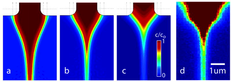
Scalar images of sample concentration (a–c). Three conditions of flow rate ratios, Qc/Qs (center channel/side channels), decreasing from left to right; from simulation. (a) Qc/Qs = 0.02 condition with center stream that is overly thick, in which mixing time is dominated by lateral diffusion in the focused stream. The concentration reaches 10% of co at x(c10%) = 22 μm downstream of the exit plane of the center nozzle. (b) An optimally sized stream, Qc/Qs = 0.01, x(c10%) = 8.2 μm, and (c) the Qc/Qs = 0.005 condition, x(c10%) = 4.3 μm, where diffusion time is again greater than optimum and dominated by the relatively slow convective diffusion process in the two-dimensional focusing region. (d) Fluorescence image from confocal scanning microscope of an optimally focused stream (with similar false color map), Qc/Qs = 0.01 and Qc ≈ 1 nL/s. The fluorescent agent is a 10 μM solution of 2 MD dextran-conjugated fluorescein in 10 mM PBS and mixing with 10 mM PBS buffer.
Perhaps the most important parameter in the problem is the ratio of the center inlet flow rate to the side inlet flow rate Qc/Qs, which can be expressed as α/β. For example, Qc/Qs determines the continuum width of the focused bulk liquid stream according to a mass flow balance:
| (9) |
so that
| (10) |
where wfs is the width of the focused stream and Ue is the centerline velocity of the exit channel. The width of the focused stream depends only on the mixer geometry and flow rate ratio of the inlet channels. Figure 3a shows how the cost function (dimensional mixing time as per eq 7) varies with Qc/Qs for α = 0.63, γ = 7.2. For Qc/Qs greater than ~0.01, mixing time is dominated by spanwise diffusion in the focused stream. For Qc/Qs less than 0.01, mixing time is dominated by two-dimensional convective diffusion in the region near the center nozzle. Qc/Qs of 0.01 results in minimum tmix = 8 μs.
Figure 3.
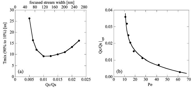
Typical results from parametric optimization study. (a) Predicted mixing time versus Qc/Qs. This ratio determines the width of the focused stream as indicated by the upper axis. The optimum flow rate ratio and stream thickness depends on the mixer geometry, absolute flow rates, and physical properties of the solutions. For α = 0.63, γ = 7.2, and Rew = 15, the optimum flow rate ratio was ~0.01, corresponding to a focused stream of 110 nm (• simulations, – straight line segment between points). (b) Dependence of optimum flow rate ratio, Qc/Qs|opt, with Peclet number. Pe number was varied by changing the diffusion coefficient alone. Each Qc/Qs|opt implies a different minimal mixing time. For solutions of iodide (PeD = 18) and guanidine (PeD = 27), there is a 26% change in the optimum flow rate ratio (• simulations, – exponential fit of the form Pe = a(b + exp((Qc/Qs)/c))).
As discussed below, we used salt ions (KI) to characterize the mixing process, but used a denaturant (GdCl) for the protein folding experiments. These two molecules have different diffusivities,49 so we investigated the effect of denaturant diffusivity on mixing time and optimal conditions. These data are plotted in Figure 3b, which shows optimal flow rate ratio as a function of Peclet number (varied by changing only diffusivity). For low diffusivity (high Pe), advection again dominates transport in the initial focusing region and so Qc/Qs should decrease to thin the center stream and maintain optimum mixing conditions.
We found dimensional mixing time increased with diffusivity for near-optimal conditions. For diffusivities, D, between 10−10 and 10−8 m2/s, a fit of the form tmix = a ln(D/Do) + b matches the predictions to within 2% (e.g., Do = 1 × 10⁻¹⁰ m2/s, a = 0.13, and b = 2.01). This counterintuitive result is due to the nonlinear effects associated with convective diffusion in the initial focusing region. Low-diffusivity denaturants enable formations of thin, low Qc center streams which have spanwise-diffusion-dominated transport and minimize tmix. High-diffusivity denaturants require relatively thick, high Qc center streams which exhibit substantial two-dimensional diffusion transport in the initial focusing region.
We also performed limited design iterations where we calculated tmix for proteins traveling through off-centerline (yp,0 ≠ 0) streamlines of the sample stream. This accounts for the slightly different Lagrangian concentration histories associated with proteins flowing along different spanwise locations in the sample stream. We found that optimal design parameters are a weak function of this initial spanwise location and so chose the centerline value as a representative case.
In general, optimal designs tended toward small nozzle dimensions and large exit velocities, and so optimal design parameters railed against the minimum feature scale and the maximum flow rate constraints described previously. Further, parametric variation of geometry for fixed values of α and γ (parameters describing geometry) show that mixing time is perhaps most sensitive to exit velocity and focused stream thickness, for the constraints considered here. A physically realizable mixer geometry had the following optimization parameters: α = 0.63, β = 20, γ = 7.2, Rew = 15, and PeDg = 800. These conditions result in a focused center stream width (neglecting molecular diffusion) of 0.11 μm and an exit velocity of Ue 2.9 m/s.
Micro-PIV
Micro-PIV measurements were taken upstream of the nozzle in each of the three inlet channels and downstream of the mixing region for several mixers in order to calibrate the applied pressure versus flow rate curves. We measured liquid velocity in the side channel regions approximately 21 μm wide and 10 μm deep. The center inlet and exit channels were measured at upstream locations where the channel cross sections were 10 μm wide and 10 μm deep. For each channel and applied pressure, velocity profiles were measured in x–y planes at three z-locations separated by 1 μm and centered about the vertical midplane (z = 0). This ensured a 1% uncertainty in maximum velocity due to height location errors. We ensemble-averaged velocity fields in correlation space for up to 100 image pairs to reduce random error due to image noise and seed particle Brownian motion. Typical correlation windows were 64 pixels × 8 pixels (12 μm × 1.5 μm; aligned along streamlines), and we used an adaptive shifting method.39 Velocity vector fields were averaged along the streamlines to produce velocity profiles. We then fit predicted analytical rectangular duct flow velocity field profiles to the measured profiles using volumetric flow rate as a fitting parameter. All of these measurements were performed at several supply pressures.
Linearity error of the pressure versus flow rate and pressure versus maximum velocity curves were typically less than 1% for a single device and less than 5% across several devices. Maximum measured flow rates and velocities in the mixing region were respectively greater than 180 nL/s and 3.0 m/s, with side inlet pressures of 400 kPa. The flow rate versus applied pressure correlations had linear coefficients of 2.02 × 10⁻¹⁰ mL s−1 Pa−1 1 (regression coefficient R2 = 0.997) and 1.56 × 10⁻¹¹ mL s−1 Pa−1 (R2 = 0.984) for the side and center inlet channels, respectively.
Dye Quenching
We performed fluorescence-quenching experiments to quantify the mixing time of our mixers. A 2-MDa dextran-conjugated fluorescein was quenched with potassium iodide. The dextran conjugated fluorescein has a diffusivity of Ddf = 7 × 10⁻¹² m2/s, compared to the iodide ion value of Diodide = 7 × 10⁻⁹ m2/s. This slowly diffusing dye follows streamlines in the times of interest, and the measurement is therefore a characterization of the rate at which iodide ions diffused into the focused stream.
We used the confocal setup to capture images of fluorescence intensity. The degree of quenching was calculated as the relative fluorescence of a quenched stream to an unquenched stream, RI = I(quenched)/I(unquenched). Measurement of RI involved careful alignment of the quenching experiment image with the unquenched image. To facilitate this alignment, we etched 1-μm indentations in the upstream channel walls that were visible under fluorescence and used as alignment marks. To further make measurements robust to alignment errors, we then averaged RI values in an area 1 μm wide and centered along the centerline. This area-averaging operation was performed using measurements spaced 0.5 μm along the streamwise direction.
The fluorescence measurements of iodide ion concentration were used to quantify mixing time. To convert these Eulerian field measurements to a Lagrangian concentration field, we used the validated velocity field model. This procedure consisted of integrating the predicted velocity field along the centerline of the focused stream, yielding a one-to-one correlation between the spatial coordinate of the measured intensity ratio, RI, and the Lagrangian time coordinate, t. A typical intensity ratio versus t curve is shown in Figure 4a. As predicted, RI is relatively constant in the initial portion of the focusing region and then drops sharply during the last stages of focusing. The signal-to-noise ratio also drops significantly at later times as the intensity of the quenched stream approached the intensity of the background noise. Also shown with the data is a low-pass-filtered version of the data calculated by convolving the raw data with a Gaussian kernel with a 0.5-μs standard deviation. The low-pass-filtered signal reaches a steady-state value in ~8 μs.
Figure 4.
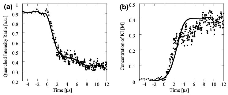
(a) Intensity ratio versus time from dye-quenching experiment. Ratio of intensity of quenched stream to an unquenched stream at same conditions. Mixing is from 0 M to 500 mM KI. Intensity ratio reaches a steady value of RI = 0.38 in 8 μs. Experimental conditions: Ue = 2.9 m/s, focused stream width 110 nm (• experiment, – low-pass filter convolution with a Gaussian kernel, σ = 0.5 μs). (b) Potassium iodide concentration as a function of time from dye-quenching experiment. Mixing is from 0 M to 500 mM KI. Salt concentration is calculated by fitting intensity ratio profile to equilibrium data. The salt concentration reaches an equilibrium value of ~400 mM in 8 μs (• experiment, – simulation).
A more direct method of measuring mixing time is given by relating RI directly to potassium iodide concentrations. This was performed by obtaining equilibrium fluorescence data in an independent experiment using a spectrofluorometer (Fluoromax-2, Jobin Yvon). A fit to the salt concentration versus intensity ratio calibration points had the form RI = a exp(bc/co), where co = 4 M is the maximum salt concentration measured and the constants a and b were respectively 0.922 and −12.4. Figure 4b shows the concentration of KI versus time from the experiment of Figure 4a, as well as results from the numerical model. The data show a Lagrangian concentration jump from 0 mM to ~400 mM potassium iodide in 8-μs mixing time.
Collapse of ssDNA with FRET
Although the previous measurements give a reasonable estimate of the mixing time of the mixer, the data are acquired in two steps and calculation of the intensity ratio may be affected by translational shifts or slight variations in the flow characteristics between the two measurements. It was therefore natural to benchmark the mixer using a FRET assay, for which it has been designed. To report on the quasi-instantaneous change of concentration of the solute diffusing from the side channel flows into the focused stream, a molecular system undergoing an even faster FRET-measurable conformational change was needed. We chose a simple model semiflexible molecule known to undergo ultrafast collapse upon transition from good to bad solvent conditions.50 The system is a short ssDNA molecule (dT30) labeled with a dye molecule at each end, transiting from a low to high salt concentration buffer. At low salt concentration, the persistence length of ssDNA (Lp = 1.5 nm) and interphosphate distance result in an extended coiled state (total contour length: L = 18 nm). In contrast, at high salt concentration, phosphate charge screening results in the collapse of the ssDNA, which adopts a condensed globule conformation.48,51 Recent Brownian dynamics simulations50 show that collapse for a short semiflexible chain of this dimension (L/Lp = 6–12) occurs in the time scale of a few hundred rotational diffusion time constants, τrot,Lp, where τrot,Lp of a rigid rod of length Lp is of the order 1 ns. This ssDNA system should thus undergo submicrosecond collapse upon transition from a low-concentration salt to a high-concentration salt environment, much faster than the mixing time already determined by the dye-quenching experiment.
We mixed 100 nM ssDNA in SM buffer with a 2 M NaCl solution in SM buffer, collecting the fluorescence signals in the donor and acceptor channel as described earlier. A typical experiment consists of simultaneously collecting a background-corrected donor image (ID) and background-corrected acceptor image (IA). We constructed a proximity ratio (PR) profile along the focused stream from the proximity ratio PR = IA/(IA + ID) of the two images, including a portion of the region preceding the mixing region for reference of the PR before mixing. PR does not report directly on FRET,52 so we used a calibration curve of PR versus [NaCl], obtained from single-molecule studies with the same sample. Figure 5a shows a typical ssDNA-FRET collapse experiment, where a change in salt concentration from 0 to ~1.5 M NaCl occurs in ~8 μs, confirming our ability to study processes occurring at time scales as small as 10 μs. The results of the numerical model are also shown in Figure 5a and agree well with the experimental data. By interrogating the downstream, exponentially diverging mixing region, we can measure long (millisecond) trajectories of the ssDNA PR. Figure 5b shows the ssDNA PR signal on a logarithmic time scale out to 10 ms with no change in PR after the initial DNA collapse, as expected.
Figure 5.
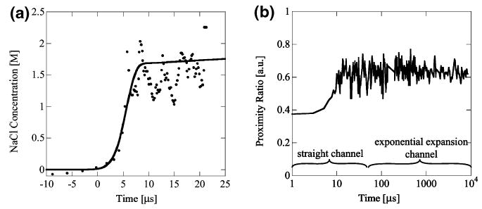
(a) Sodium chloride concentration versus time from single-stranded DNA collapse experiment. Salt concentration obtained from fit of FRET ratio calibration using equilibrium data. Mixing was from 0 to 2 M NaCl and was complete within ~8 μs. Experimental conditions: Ue = 2.9 m/s, focused stream width 110 nm (• experiment, – simulation). (b) Long time scale of ssDNA collapse experiment. Mixing of FRET labeled ssDNA from 0 to 2 M NaCl. The short time scale (<10 μs) kinetics of the DNA collapse are captured along with the long time scale, up to 10 ms in the exponentially expanding exit channel. No subsequent change in PR is detected after the initial collapse as expected.
Resolving Collapse of ACBP
ACBP folding was previously characterized in a continuous-flow mixer apparatus by Teilum et al. 45 Their experiments indicate that ACBP folds via a presumably on-pathway folding intermediate (U ↔ I ↔ N), with rate constants of approximately 80 μs and 2–10 ms for the formation of the collapsed intermediate (I) and its decay into the native state (N), respectively. We monitored refolding of ACBP via FRET between two extrinsic dyes attached to the N- and C-termini, respectively. Both termini are solvent-accessible, and charged dyes with C2-or C5-linkers are used, affording maximal rotational freedom of the chromophores and minimal interaction with the protein. The change in the PR upon dilution of denatured ACBP (6 M GdCl) into aqueous buffer is clearly biphasic, as shown in Figure 6. About 50% of the expected PR amplitude (PR difference between unfolded and native protein) is gained in a fast process, indicating significant chain compaction within the first 200 μs of folding (Figure 6a). Complete recovery of the native PR signal is achieved in a slower step in the millisecond time range, as shown in Figure 6b. Fitting of the kinetic trace to a sum of two exponentials of the form PR-(t) = A1 + A2e−t/A3 + A4e−t/A5 yielded rate constants (with standard errors) of A3 = 92 ± 9.4 μs and A5 = 8.5 ± 1.6 ms for the fast and slow phases, respectively (A1 = 0.522, A2 = 0.297, A4 = 0.134). The fit has a nonlinear regression coefficient value of R2 = 0.964. These two measured rate constants agree well with the respective values of 80 μs and 9 ms published by Teilum.45
Figure 6.
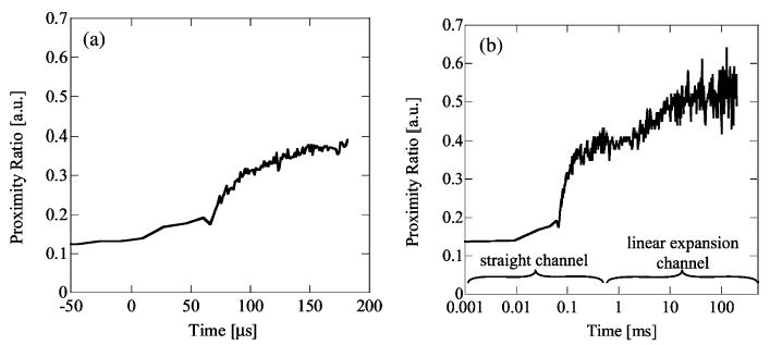
(a) Proximity ratio versus time from ACBP folding experiment. Mixing denatured ACBP from 6 to 0 M guanidine. The decrease in denaturant concentration induces the folding kinetics of the protein. A proximity ratio change is observed at ~90 μs, indicating a fast collapse phase of the protein in good agreement with previous reports. (b) ACBP FRET experiment showing proximity ratio plotted on logarithmic time axis. Since the fluid flow slows down in the linearly expanding exit region, a single experiment can record time scales from 10 μs to over 100 ms. The measured proximity ratio indicates a fast kinetic response at 90 μs and a slower kinetic response at 8 ms.
CONCLUSIONS
Two major barriers in studying protein folding with continuous-flow mixing methods have been long mixing times, due to physical limits of material line stretching and diffusion, and large sample consumptions. A recently proposed solution to these barriers is the use of hydrodynamic focusing to reduce diffusion distances and mixing times. We have sought to optimize a microfluidic mixer that utilizes hydrodynamic focusing in order to push the limits of time resolution in protein folding studies, while consuming minimal amounts of protein sample.
We modeled mixing dynamics and optimized mixing performance using dimensionless Navier–Stokes and convective–diffusion equations, reducing the important independent variables to five nondimensional parameters describing mixer geometry, flow conditions, and thermophysical properties. The problem’s cost function was defined as the time required for the Lagrangian reference frame concentration to drop a specified amount. We used a parametric approach, varying five nondimensional parameters independently, to find a minimum of the cost function and identify the degree of sensitivity to various parameters.
This optimization approach led to a mixer design with small nozzle widths constrained by fabrication techniques to ~1 μm, a large exit flow rate constrained by Reynolds number and consideration of clogging issues, and an optimal focused stream width that depended on the mixer geometry and flow rates. This led to the counterintuitive results that a narrower focused stream does not always mix faster and that lower diffusivity denaturants can lead to lower mixing times. We propose an explanation for these results by taking into account the multidimensional convective–diffusion effects in the focusing region.
Mixers were batch-fabricated using standard microfabrication techniques on silicon substrates. We used micro-PIV to calibrate the applied pressures to flow rate relations and quantify velocities in the mixer. The fast reaction kinetics of fluorescence quenching and ssDNA collapse were used to characterize mixer response time; these measurements demonstrate mixing times of less than 10 μs and agree well with a numerical model. Finally, we measured the kinetic rates of a benchmark protein, ACBP, to show feasibility in studying protein folding on fast time scales.
We have developed the fastest reported continuous-flow microfluidic mixer for studying protein folding and have measured mixing times of less than 8 μs. Our mixer is reliable, yields repeatable results, is easy to batch-fabricate, and consumes very small amounts of precious sample. This mixer enables the study of submicrosecond kinetics of protein folding and other fast biochemical processes.
Acknowledgments
We thank Brian Campbell of UCLA for help with the optical setup and Jane Bearinger of LLNL and Stephanie Pasche of ETH, Zurich, for supplying the PLL-g-PEG. This work was performed under the auspices of the U.S. Department of Energy under Contract W-7405-Eng-48 with funding from the LDRD program. The support of NIH (Grant 1R01-GM65382) to S.W.’s group is gratefully acknowledged. Support by NIH (Grant N01-HV-28183) to J.G.S.’s group is also gratefully acknowledged.
References
- 1.Roder H. Proc Natl Acad Sci USA. 2004;101:1793–1794. doi: 10.1073/pnas.0308172101. [DOI] [PMC free article] [PubMed] [Google Scholar]
- 2.Jones CM, Henry ER, Hu Y, Chan CK, Luck SD, Bhuyan A, Roder H, Hofrichter J, Eaton WA. Proc Natl Acad Sci USA. 1993;90:11860–11864. doi: 10.1073/pnas.90.24.11860. [DOI] [PMC free article] [PubMed] [Google Scholar]
- 3.Hagen SJ, Eaton WA. J Mol Biol. 2000;301:1037–1045. doi: 10.1006/jmbi.2000.3969. [DOI] [PubMed] [Google Scholar]
- 4.Pryse KM, Bruckman TG, Maxfield BW, Elson EL. Biochemistry. 1992;31:5127–5136. doi: 10.1021/bi00137a006. [DOI] [PubMed] [Google Scholar]
- 5.Jacob M, Holtermann G, Perl D, Reinstein J, Schindler T, Geeves MA, Schmid FX. Biochemistry. 1999;38:2882–2891. doi: 10.1021/bi982487i. [DOI] [PubMed] [Google Scholar]
- 6.Chan CK, Hu Y, Takahashi S, Rousseau DL, Eaton WA. Proc Natl Acad Sci USA. 1997;94:1779–1784. doi: 10.1073/pnas.94.5.1779. [DOI] [PMC free article] [PubMed] [Google Scholar]
- 7.Pollack L, Tate MW, Darnton NC, Knight JB, Gruner SM, Eaton WA, Austin RH. Proc Natl Acad Sci USA. 1999;96:10115–10117. doi: 10.1073/pnas.96.18.10115. [DOI] [PMC free article] [PubMed] [Google Scholar]
- 8.Park SH, Shastry MCR, Roder H. Nat Struct Biol. 1999;6:943–947. doi: 10.1038/13311. [DOI] [PubMed] [Google Scholar]
- 9.Shastry MCR, Luck SD, Roder H. Biophys J. 1998;74:2714–2721. doi: 10.1016/S0006-3495(98)77977-9. [DOI] [PMC free article] [PubMed] [Google Scholar]
- 10.Magg C, Schmid FX. J Mol Biol. 2004;335:1309–1323. doi: 10.1016/j.jmb.2003.11.050. [DOI] [PubMed] [Google Scholar]
- 11.Schuler B, Lipman EA, Eaton WA. Nature. 2002;419:743–747. doi: 10.1038/nature01060. [DOI] [PubMed] [Google Scholar]
- 12.Lipman EA, Schuler B, Bakajin O, Eaton WA. Science. 2003;301:1233–1235. doi: 10.1126/science.1085399. [DOI] [PubMed] [Google Scholar]
- 13.Brody JP, Yager P, Goldstein RE, Austin RH. Biophys J. 1996;71:3430–3441. doi: 10.1016/S0006-3495(96)79538-3. [DOI] [PMC free article] [PubMed] [Google Scholar]
- 14.Stroock AD, Dertinger SKW, Ajdari A, Mezic I, Stone HA, Whitesides GM. Science. 2002;295:647–651. doi: 10.1126/science.1066238. [DOI] [PubMed] [Google Scholar]
- 15.White F. M: Viscous Fluid Flow; McGraw-Hill: New York, 1991.
- 16.Akiyama S, Takahashi S, Ishimori K, Morishima I. Nat Struct Biol. 2000;7:514–520. doi: 10.1038/75932. [DOI] [PubMed] [Google Scholar]
- 17.Akiyama S, Takahashi S, Kimura T, Ishimori K, Morishima I, Nishikawa Y, Fujisawa T. Proc Natl Acad Sci USA. 2002;99:1329–1334. doi: 10.1073/pnas.012458999. [DOI] [PMC free article] [PubMed] [Google Scholar]
- 18.Pollack L, Tate MW, Finnefrock AC, Kalidas C, Trotter S, Darnton NC, Lurio L, Austin RH, Batt CA, Gruner SM, Mochrie SGJ. Phys Rev Lett. 2001;86:4962–4965. doi: 10.1103/PhysRevLett.86.4962. [DOI] [PubMed] [Google Scholar]
- 19.Kauffmann E, Darnton NC, Austin RH, Batt C, Gerwert K. Proc Natl Acad Sci USA. 2001:6646–6649. doi: 10.1073/pnas.101122898. [DOI] [PMC free article] [PubMed] [Google Scholar]
- 20.Russell R, Millett IS, Tate MW, Kwok LW, Nakatani B, Gruner SM, Mochrie SGJ, Pande V, Doniach S, Herschlag D, Pollack L. Proc Natl Acad Sci USA. 2002;99:4266–4271. doi: 10.1073/pnas.072589599. [DOI] [PMC free article] [PubMed] [Google Scholar]
- 21.Pabit SA, Hagen SJ. Biophys J. 2002;83:2872–2878. doi: 10.1016/S0006-3495(02)75296-X. [DOI] [PMC free article] [PubMed] [Google Scholar]
- 22.Knight JB, Vishwanath A, Brody JP, Austin RH. Phys Rev Lett. 1998:3863–3866. [Google Scholar]
- 23.Fox MH, Manney TR. Cytometry. 1981;2:98–98. [Google Scholar]
- 24.Hur JS, Shaqfeh ES, Babcock HP, Chu S. Phys Rev E. 2002;66:011915. doi: 10.1103/PhysRevE.66.011915. [DOI] [PubMed] [Google Scholar]
- 25.Wang J. Electrophoresis. 2002;23:713–718. doi: 10.1002/1522-2683(200203)23:5<713::AID-ELPS713>3.0.CO;2-7. [DOI] [PubMed] [Google Scholar]
- 26.Darnton N, Bakajin O, Huang R, North B, Tegenfeldt J, Cox E, Sturn J, Austin RH. J Phys : Condens Matter. 2001;13:4891–4902. [Google Scholar]
- 27.Probstein R. F: Physicochemical Hydrodynamics; John Wiley and Sons: New York, 1994.
- 28.Munson MS, Cabrera CR, Yager P. Electrophoresis. 2002;23:2642–2652. doi: 10.1002/1522-2683(200208)23:16<2642::AID-ELPS2642>3.0.CO;2-P. [DOI] [PubMed] [Google Scholar]
- 29.Ottino J. M: The Kinematics of Mixing: Stretching, Chaos, and Transport; Cambridge University Press: Cambridge, U.K., 1989.
- 30.Munson MS, Yager P. Anal Chim Acta. 2004;507:63–71. [Google Scholar]
- 31.Panic S, Loebbecke S, Tuercke T, Antes J, Boskovic D. Chem Eng J. 2004;101:409–419. [Google Scholar]
- 32.Aref H, Naschie M. S. E: Chaos Applied to Fluid Mixing; Pergamon: New York, 1995.
- 33.Sawhney AS, Hubbell JA. Biomaterials. 1992;13:863–870. doi: 10.1016/0142-9612(92)90180-v. [DOI] [PubMed] [Google Scholar]
- 34.Elbert DL, Hubbell JA. Biomed Mater Res. 1998;42:55–65. doi: 10.1002/(sici)1097-4636(199810)42:1<55::aid-jbm8>3.0.co;2-n. [DOI] [PubMed] [Google Scholar]
- 35.Kenausis GL, Voros J, Elbert DL, Huang N, Hofer R, Ruiz-Taylor L, Textor M, Hubbell JA, Spencer ND. J Phys Chem B. 2000;104:3298–3309. [Google Scholar]
- 36.Bearinger JP, Voros J, Hubbell JA, Textor M. Biotechnol Bioeng. 2003;82:465–473. doi: 10.1002/bit.10591. [DOI] [PubMed] [Google Scholar]
- 37.Santiago JG, Wereley ST, Meinhart CD, Beebee DJ, Adrian RJ. Exp Fluids. 1998;25:316–319. [Google Scholar]
- 38.Devasenathipathy S, Santiago JG, Wereley ST, Meinhart CDKT. Exp Fluids. 2003;34:504–514. [Google Scholar]
- 39.Wereley ST, Meinhart CD. Exp Fluids. 2001;31:258–268. [Google Scholar]
- 40.Kamholz AE, Weigl BH, Finlayson BA, Yager P. Anal Chem. 1999;71:5340–5347. doi: 10.1021/ac990504j. [DOI] [PubMed] [Google Scholar]
- 41.Oddy MH, Santiago JG, Mikkelsen JC. Anal Chem. 2001;73:5822–5832. doi: 10.1021/ac0155411. [DOI] [PubMed] [Google Scholar]
- 42.Lakowicz J. R: Principles of Fluorescence Spectroscopy, 2nd ed., Kluwer Academic/Plenum Publishers: New York, 1999.
- 43.SM buffer. 20 mM TRIS, pH 8, 1 mM mercaptoethylamine, 100 M EDTA, and NaCl ranging from 0 mM to 2 M.
- 44.Laurence, T. L., Kong, X., Weiss, S. Unpublished work, UCLA, 2004.
- 45.Teilum K, Maki K, Kragelund BB, Poulsen FM, Roder H. Proc Natl Acad Sci USA. 2002;99:9807–9812. doi: 10.1073/pnas.152321499. [DOI] [PMC free article] [PubMed] [Google Scholar]
- 46.Lacoste TD, Michalet X, Pinaud F, Chemla DS, Alivisatos AP, Weiss S. Proc Natl Acad Sci USA. 2000;97:9461–9466. doi: 10.1073/pnas.170286097. [DOI] [PMC free article] [PubMed] [Google Scholar]
- 47.Excitation XDM; emission EDM. TMR/Alexa 647. laser, 514 nm; XDM = 540DRLP; EDM = 625DRLP; donor EF, 580DF60; acceptor EF, HQ650LP + SP750. Alexa 488/Alexa 647: laser, 488 nm; XDM = 500DCXT; EDM = 625DRLP; donor EF, 530DF50; acceptor EF, HQ650LP + SP750.
- 48.Murphy MC, Rasnik I, Cheng W, Lohman TM, Ha T. Biophys J. 2004;86:2530–2537. doi: 10.1016/S0006-3495(04)74308-8. [DOI] [PMC free article] [PubMed] [Google Scholar]
- 49.D(iodide)/D(guanidine) = 2.
- 50.Montesi A, Pasquali M, MacKintosh FC. Phys Rev E. 2004;69:021916. doi: 10.1103/PhysRevE.69.021916. [DOI] [PubMed] [Google Scholar]
- 51.Deniz AA, Laurence TA, Dahan M, Chemla DS, Schultz PG, Weiss S. Annu Rev Phys Chem. 2001;52:233–253. doi: 10.1146/annurev.physchem.52.1.233. [DOI] [PubMed] [Google Scholar]
- 52.PR depends on detection efficiency in the two channels, donor leakage in the acceptor channel and direct excitation of the acceptor.