

Abstract
We outline a theoretical treatment that describes fibril formation in dilute protein solutions. For this, we combine a theory describing self-assembly and conformational transition with a description of the lateral association of linear chains. Our statistical-mechanical model is able to predict the mean degree of polymerization and the length of the fibrils and their precursors, as well as the weight fractions of the different aggregated species in solution. We find that there appear to exist two regimes as a function of concentration, and as a function of the free energies of protein association: one in which low-molecular weight compounds dominate and one in which the fibrils do. The transition between these regimes can be quite sharp, and becomes sharper as more filaments are allowed to associate into a single fibril. The fraction of fibrils consisting of less than the maximum allowed number of filaments turns out to be negligible, in agreement with experimental studies, where the fibril thickness is found to be practically monodisperse. In addition, we find that the description of the fibril ends has a large effect on the predicted fibril length.
INTRODUCTION
The self-assembly of naturally occurring, water-soluble protein molecules into fibrous material (amyloid fibril formation) and the subsequent precipitation of these fibrils are common elements in a host of diseases. Prime examples include Alzheimer's and Parkinson's diseases and prion-related disorders (1–10). Besides the impact that this type of biomolecular self-assembly has on issues in disease study and prevention, the field has recently experienced a surge in interest from the area of materials science (11–13). This is because the properties of the assemblies are potentially adjustable by changing environmental factors such as pH or temperature, the range of structures they can form is very large, and their biological origin may allow their use in living organisms. To better understand the mechanisms behind the fibrillogenesis, many experimental (5,10,14–21) and computational studies (6,8,22,23) have been performed recently.
Amyloidosis is a phenomenon observed in many proteins under different conditions, seemingly independent of the exact composition of the protein molecules (1,2,4,16,24). Hence, it seems plausible that a general mechanism controls the fibril formation. We therefore propose a general theoretical treatment for this fibrillogenesis, valid for dilute solutions (i.e., we assume that the fibrils and their precursors do not interact appreciably with each other). By focusing on the common features of the fibril formation, we necessarily neglect many of the structural details of specific amyloid fibrils. These may differ from protein to protein (23). If one wishes to give a more detailed description of the fibril structure for a specific protein, however, such details may easily be incorporated into the theoretical framework presented here.
Our treatment is not the first theoretical study of protein fibrillogenesis. Earlier studies include the Oosawa-Kasai model (25–27) and the more recent model of Nyrkova and co-workers (11). Our model is a combination and an extension of these two theories. Specifically, we apply a recent extension (beyond the all-or-nothing case) of the Oosawa theory of two-state, linear assembly into filaments (26–29). We then combine this approach with the description of lateral assembly of filaments as applied by Nyrkova et al. (11). This yields a quasi-one-dimensional model that can be resolved analytically and that gives results that are exact within the model assumptions.
The remainder of this article is organized as follows. In the Theory section, we outline our model and present the equations that describe the fibril formation. We also introduce three sets of boundary conditions describing the fibril ends, and go on to show in Results that the choice of boundary conditions has a potentially large effect on the predicted fibril properties. In this section, we also discuss our prediction of the mean fibril length, the fraction of protein molecules present as monomers, dimers, filaments, and fibrils, and the fraction of proteins in a β-strand conformation, as a function of the protein concentration and the free energies of interaction. We find that there is a sharp transition between a fibril-dominated regime at high concentration and a regime dominated by monomers and small aggregates at low concentration. Similar results are obtained as a function of the various binding free energies. Finally, we give our conclusions and outlook in the last section, remarking on the applicability of our model and the steps necessary to present a comparison between the theory and experimental results.
THEORY
To write down a theory for amyloid fibril formation in dilute solution, we must take the following general characteristics account. Firstly, it is known that the fibrils have a well-defined diameter and that they consist of several intertwined filaments (4,8,24): for the 42-residue Aβ peptide (a protein linked to Alzheimer's disease), e.g., the fibrils are believed to be made up of five or six filaments (3,8,20). Inside the fibrils, protein molecules possess a β-strand conformation, which allows them to form long intermolecular β-sheets (known as cross-β-sheets). Secondly, so-called protofibrils and protofilaments are known to play a role in the amyloidosis. The former species is defined as a semifibrillar aggregate that plays a role early in the amyloid fibril formation, whereas the latter is a component of the mature fibrils, i.e., an amyloid fibril is believed to be composed of several protofilaments (4,20,24). Finally, it is well established that nucleation is an important factor in fibrillogenesis (1,4,17,26,30,31). (We assume here that the formation of protofibrils and protofilaments is a reversible process. This need not be so for all proteins. The consequences of this are discussed in Conclusions and Outlook. In classical nucleation and growth, an unstable intermediate (the nucleus) plays an important role. Our treatment is unsuited to describe the dynamics of this process, but we can describe the resulting stable fibrils. This, too, is discussed in Conclusions and Outlook.)
We outline below a model that combines these characteristics, shown in Fig. 1. Here, blobs represent monomers in a disordered conformation, and disks represent proteins in a β-strand-type conformation. The disk representation was chosen for convenience, and is not meant to imply that these molecules possess a cylindrical symmetry. We regard the monomeric protein molecules as being in a disordered state, which we need not specify further. These molecules can associate into dimers and filaments through a relatively weak and reversible physical interaction. This association may be due to, for instance, hydrophobic interactions, hydrogen bonding, electrostatic interactions, or a combination of such contributions. We presuppose that two types of association can exist between protein molecules, one that has a β-sheet-like character, and one that has a less ordered (non-β) character. The former type of interaction is required because amyloid fibrils are known to possess a cross-β-sheet structure, as mentioned above, and we include the latter type of interaction because it has been speculated that (partially) disordered aggregates may form for some amyloid-forming proteins (6,19,21,23). We assume that dimers contain only the latter, relatively unfavorable, type of association. This ensures that β-type associations (and the accompanying cross-β-sheets) only form in larger aggregates. We make this assumption because cross-β-sheets are known to only become stable if they contain a sufficient number of monomers. In the larger linear assemblies (the filaments), each monomer-monomer interaction (except the filament ends, which shall be discussed in some detail below) can have either a β-type character, if both molecules have a β-strand-type conformation, or a disordered character, if this is not so.
FIGURE 1.

Schematic representation of the aggregated states. In the first step monomers aggregate into filaments with a variable β-sheet content (two examples are shown). These filaments assemble into fibrils in the second step (two examples of fibrils are shown, one containing six filaments of equal length and one containing two filaments of unequal length). Blobs indicate protein molecules in a non-β-state, whereas disks represent proteins in a β-conformation.
Completing our description of the aggregated states, we describe the fibrils (which consist of several laterally associated filaments) as comprising two parts: the “body”, which we assume consists entirely of protein molecules in a β-strand conformation (based on experimental evidence of high β-sheet content in the fibrils), and the “loose ends” or “legs” (11), which make up the ends of the fibrils, and which we treat as comprising monomers in the disordered, non-β-state. This is discussed in more detail below, in the Fibrils section. We furthermore assume that the filaments and fibrils are rigid structures, i.e., that they do not fold back upon themselves.
Note that in our description, filaments directly combine to form a fibril, without any intermediate steps. For many proteins, this process is somewhat more complex, as the protofilaments that combine to form the fibril may themselves consist of several intertwined filaments (24). However, there also exist proteins for which the fibril formation is believed to conform to our description (24). With some slight adjustments, our theoretical framework should be able to describe the more complex case as well.
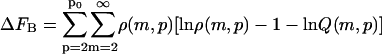
The overall free energy per unit volume of a solution of self-assembling material, ΔF, can be written as (11,33)
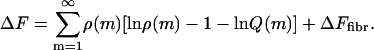 |
(1) |
Here, ΔF is given in units of thermal energy, kBT, with kB Boltzmann's constant and T the absolute temperature. The same is true for all (free) energies used throughout this article, unless explicitly noted otherwise. In Eq. 1, ρ(m) is the dimensionless number density of (linear) aggregates of degree of polymerization m, Q(m) is their (canonical) partition function, and ΔFfibr is the free-energy term for fibrils, to be detailed below in the Fibrils section. From Eq. 1, we can calculate the equilibrium size distribution by setting the functional derivative of the free energy with regards to the number density ρ of any species (monomers, dimers, filaments, or fibrils) equal to zero, while enforcing conservation of mass. It turns out that the equilibrium size distribution of each species equals its partition function, multiplied by the exponent of μN, with N the number of protein molecules that make up the aggregate and μ a Lagrange parameter that we interpret as the (dimensionless) chemical potential of the protein molecules. Now, to establish the properties of the protein assemblies, we need to first determine the partition functions for the monomeric, dimeric, filament, and fibril states.
Monomers and dimers
Because monomers are not involved in any associations, we set their dimensionless Hamiltonian H(1) equal to zero, so that it acts as a reference level. The partition function of the monomers, Q(1), is then equal to unity.
As mentioned above, we consider the dimers to consist of two disordered molecules linked by a single interaction, with free energy M. The Hamiltonian of a dimer is therefore H = M, and its partition function becomes Q(2) = k ≡ exp −M. Note that we ignore here any change of the conformational state that may take place upon association, i.e., the difference between the conformation of a protein molecule as a free monomer and the same molecule bound in a dimer. This assumption avoids the introduction of another free-energy parameter (as we shall discuss below, the problem at hand already requires four such parameters) and is not too severe, because the energy that accompanies this conformational transition only shifts the binding energy by a fixed amount (albeit, strictly speaking, only in the infinite-chain limit). Additionally, Nyrkova and co-workers show that, at least for the DN1 protein they study (a protein that shows a similar fibril formation), the free energy of this conformational transition is significantly smaller than that of a monomer-monomer interaction (11).
Filaments
To describe the properties of the filaments, we apply a quasi-one-dimensional two-state model (28). This model, which combines a model for linear self-assembly (33) with one for a conformational transition (34), was recently successfully applied in a description of the helical self-assembly of disk-shaped molecules (28,35). We introduce two free-energy parameters, in addition to the free energy for the formation of an association between two monomers, M, given in the previous paragraph: the excess free energy if both those monomers are in a β-strand conformation, P (this measures the difference between the interaction in a cross-β-sheet with free energy P* = P + M and that in a disordered aggregate with free energy M), and the free-energy penalty associated with a “frustrated” monomer, i.e., a protein molecule that is bound to one of its neighbors with a β-type association, and to the other with a non-β-type association, R (this can also be seen as the free-energy penalty of an “interface” between a β-sheet region and a disordered region along the aggregate axis). These free energies are illustrated in Fig. 2 (also included here is the free energy F, needed to describe fibril formation. This parameter is described in the next subsection). Note that the free energy of the conformational transition of a monomer inside a filament, from a disordered state to a β-strand one, is not explicitly taken into account here. Doing so would introduce another free-energy parameter, which only renormalizes the parameters P and R.
FIGURE 2.

Schematic depiction of the free-energy parameters applied in our model. M is the (reference) association energy, P* = P + M is the free energy for the interaction between two monomers in a β-strand conformation, R is the free-energy penalty on the formation of an “interface” between an ordered and a disordered region, and F is the lateral interaction free energy.
We can now write down the dimensionless Hamiltonian Hfil needed to describe filaments longer than two monomers. It equals (29)
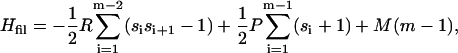 |
(2) |
where m gives again the number of protein molecules in the filament, and si denotes the nature of each association; it has a value of unity if the interaction is ordered in nature, (i.e., both monomers have a β-strand conformation) and −1 otherwise. The Hamiltonian Eq. 2 corresponds to that of the Ising chain, with P corresponding to the magnetic-field strength, si to the spin value, and R to the spin-spin interaction.
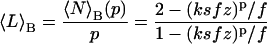
To determine the partition function from the Hamiltonian, we apply the well-known transfer matrix method (28,29,34,36). This means that we define a matrix that gives the unnormalized probabilities (Boltzmann weights) of each type of interaction, given the type of association that precedes it. The method allows for a relatively easy way to calculate the partition function via the eigenvalues of this matrix. The transfer matrix takes the form
 |
(3) |
Here, ann gives the Boltzmann weight of a non-β-association (the interaction that exists between two proteins that are not both in a β-strand conformation) that follows a non-β-association, anβ gives that of a non-β-association after a β-association, aβn that of a β-association after a non-β-association, and aββ that of a β-association after another β-association. If we use the non-β bound state as the reference state and insert unity for a non-β-association, s ≡ exp −P for a β-interaction, and  for a monomer that is bound in a non-β way on one side, and in a β-way on the other, we obtain (28,34,35)
 |
(4) |
The partition function of a filament with degree of polymerization m is now given by
 |
(5) |
Here, the vectors u and u+ describe the ends of the filaments,
 |
(6) |
 |
(7) |
with un the unnormalized probability for the last protein-protein interaction of the filament to have a non-β-character, u′n the Boltzmann weight for the first such interaction of the aggregate to be in a non-β-state, and uβ and u′β the same for the β-state. The evaluation of Eq. 5 is simplified if we diagonalize the transfer matrix,  with Λ the diagonalized matrix containing the eigenvalues of M, T the matrix of column eigenvectors
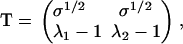 |
(8) |
and T−1 its inverse (35). The eigenvalues of M equal  where the + symbol gives λ1 and the − symbol λ2 (27,33,34).
Now we need to specify the vectors that describe the filament ends. We can impose one of three sets of boundary conditions (see van Gestel et al. (29) for a detailed description). In the first, we allow the first and last interactions of each filament to have a non-β or a β-character. The vectors u and u+ then become (1 1) and (1 s)+. In the second, we constrain these associations to be of the non-β-type. This means that we set uβ and u′β equal to zero, so that the vectors become (1 0) and (1 0)+. Similarly, we can fix the ends to be in a β-type conformation, with vectors (0 1) and (0 s)+.
That the choice of boundary conditions affects the conformational state and mean length of helical self-assembled chains, has been described in recent work (29). In this work, we set the first and last monomer of the filaments to be in a non-β-state, an end description that corresponds to setting s1 and sm-1 both equal to −1 in Eq. 2. Our reason for doing so is, as mentioned above, that this choice enables us to take into account the circumstance that cross-β-sheets are only stable if they contain a large enough number of molecules. Employing Eq. 5 to calculate the partition function, we obtain
 |
(9) |
In Eq. 9, k is again the Boltzmann factor of a disordered-type interaction, and x and y are prefactors dependent on the boundary conditions; for the end description we apply, they equal  and
and  (29).
(29).
Fibrils
To describe the fibrils, we include lateral interactions between the filaments. This technique is known to provide a good description of the self-assembly of the 11-residue DN1 polypeptide (11). In addition to the three free-energy parameters described in the previous subsection, we now require a fourth parameter, the free energy of a single lateral interaction, F, which describes the strength of the interfilament associations inside a fibril (see Fig. 2).
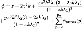
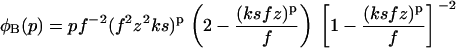
The Hamiltonian of a fibril depends on the state of its ends, as does the form of ΔFfibr in Eq. 1. In Nyrkova et al (11), the possibility is suggested that the filaments that make up the fibril need not have the same length, and hence, the fibril may have some “loose ends” or “legs”. In our model, we can also take these into account, and describe them as linear stretches of proteins in a non-β conformation (case A). Earlier studies have led to speculation that amyloid fibrils, may, indeed, have partially unfolded ends. (4) Alternatively, we can fix the last monomer of the fibrils to be in a β-strand conformation, effectively defining that the fibrils comprise solely proteins in a cross-β-sheet conformation (case B). It is also possible to allow the fibril ends to attain either of these states. In this latter case, which we shall refer to as case C, we restrict the length of any “loose ends” to a single monomer, for computational reasons. (We can also define a model in which the loose ends can have any length from zero to infinity by the application of a Dirac δ-function, which gives a value of unity if the length of a loose end equals zero, and zero otherwise. However, we expect this to yield similar results to the model C as defined in the text, and this latter model is likely easier to resolve analytically.) That this is reasonable follows from the work of Nyrkova and co-workers, who find that for realistic values of the free-energy parameters, the mean length of the loose ends becomes less than a single monomer (11).
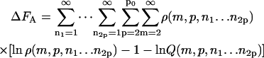
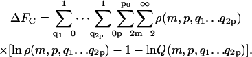
The parameter ΔFfibr, giving the total free energy of fibrils in dilute solution, (see Eq. 1) equals ΔFA, ΔFB, or ΔFC depending on the boundary conditions:
 |
(10) |
 |
(11) |
 |
(12) |
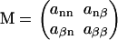
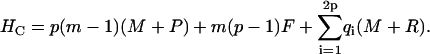
Here, m is the number of protein molecules per filament that make up the fibril “body”, p equals the number of filaments that comprise a fibril, with p0 its upper boundary enforced by the architecture of the fibrils, ni > 0 gives the number of monomers present in the “leg” numbered i, whereas qi gives the same, however limited to a value of zero or unity. The Hamiltonians for the three cases are as follows.
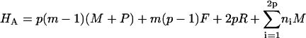 |
(13) |
 |
(14) |
 |
(15) |
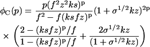
We obtain the following partition functions from the Hamiltonians Eqs. 13–15 for fixed m, p, and “loose end” length.
 |
(16) |
 |
(17) |
 |
(18) |
In Eqs. 16–18, f ≡ exp −F is the Boltzmann factor for lateral binding of filaments; k gives again the Boltzmann factor for the formation of a non-β association, and s that of the transition of a non-β-type interaction to a β-type interaction, whereas σ gives the square of the Boltzmann factor for an interface between a non-β and a β-region along the fibril axis, also as before.
Note that the fibrils we discuss here are actually sheet-like in structure. To describe proper fibrils, the last filament would have to bind to the first one, closing the circle and thus forming a cylindrical aggregate. We may naively include such a final interfilament interaction in an easy way by setting the lateral-binding term in the Hamiltonians Eqs. 13–15 equal to mpF. This, however, is an approximation, as it implies that neither the difference in entropy between a sheet and a cylindrical aggregate, nor elastic energies, play a role in the ring closure. In the results section, we shall highlight the differences between the sheet-like and the cylindrical conformations for large fibrils (p > 2), and show that this approximation is in fact a severe one.
Overall properties
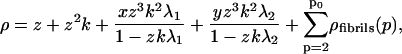
Now that we have established the partition functions, we can calculate the overall properties of a dilute solution of assembling protein molecules. Let us first focus on the overall size distribution ρ, obtained by adding the number densities of monomers, dimers, filaments, and fibrils. The number densities of monomers and dimers are equal to 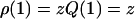 and
and  with Q(1) and Q(2) given in the “Monomers and dimers” section, and with z ≡ exp μ a fugacity. To determine the number density of filaments, we need to perform a summation of
  over all values of m. Because monomers and dimers are treated separately, we sum from m = 3 to m = ∞. Similarly, we can determine the total number of fibrils per unit volume by summing over the relevant values of p, m, ni, and qi, taking care to include a fugacity term for each of the protein molecules present in the fibrils. The limits of these summations are the same as those seen in Eqs. 10–12. This gives for the overall size distribution
 |
(19) |
with the fibrillar terms given by
 |
(20) |
 |
(21) |
 |
(22) |
Here we have not yet evaluated the summation over p (see Eqs. 10–12), because its upper bound depends on the protein being considered. For Aβ1-42 protein, e.g., as mentioned above, it is known that p0 most likely equals five or six (3,8,20,31), but other values have been found for different proteins (1,23). The reason why well-defined fibrils consisting of a fixed number of filaments are formed is unknown, but believed to be related to the architecture of the fibrils, most notably to the asymmetry of their building blocks, and the inherent twist of the filaments.
Next, we calculate the total number of protein molecules per volume unit in solution. This volume fraction φ is given by the product of the number of protein units in a given assembly and the dimensionless amount of that particular assembly per unit volume, subsequently summed over all aggregate sizes (28,29,35). It equals
 |
(23) |
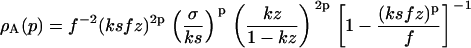
with φfibrils given for the boundary conditions A, B, and C by
 |
(24) |
 |
(25) |
 |
(26) |
(Note that, in order for the volume fraction φ to be finite, the combinations of parameters zkλ1, zkλ2 and (ksfz)p/f must each have a value smaller than unity.) Now, by dividing the volume fraction of monomers, φ(1) = z, by the total volume fraction, we can determine which mass fraction of proteins is in the monomeric state. We can determine the mass fraction of the other assemblies in the same way.
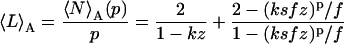
Another important quantity we can now determine is the mean degree of polymerization. It is defined as
 |
(27) |
Complimentary to this overall mean aggregate size, we can find the mean degree of polymerization of filaments and fibrils by dividing the total number of protein molecules that make up the aggregates of that type by the number of those aggregates. Their mean lengths can then be found by dividing the mean degree of polymerization of the fibrils by the number of filaments they contain. By extension, this means that the mean length of the filaments is equal to their degree of polymerization, and is given by
 |
(28) |
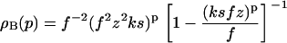
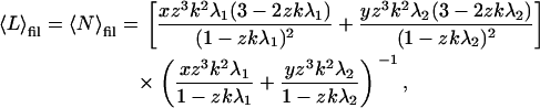
whereas that of the fibrils becomes
 |
(29) |
 |
(30) |
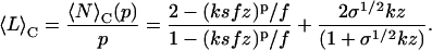 |
(31) |
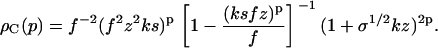
Finally, we can use standard statistical-mechanical techniques to determine the mean fraction of monomers in a β-strand conformation, averaged over all aggregate sizes and conformations. It is given by (for case A)
 |
(32) |
Here, the terms for monomers and dimers are omitted, because these species cannot contain any β-type associations in our model. For case C, the summations over ni would be replaced by those over qi, running from zero to unity, whereas for case B the dependence on ni, as well as the corresponding summations, would be absent. In Eq. 32, θ is the fraction of β-type interactions in a single filament or fibril. For the filaments it is given by
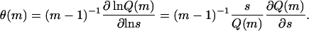 |
(33) |
This can be understood if one realizes that the derivative after the first equal sign corresponds to the number of times the free energy of a β-type interaction occurs in the total free energy of the filament. This equals the number of interactions that have a β-character. The fraction of these associations is then obtained by division by the total number of interactions, m − 1.
For a fibril, θ depends on the boundary conditions. It can readily be determined by counting the number of interactions along the fibril axis in the “body” of the fibril (because these are defined to have a β-character), and dividing this number by the total number of associations, i.e., it equals 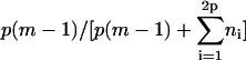 for case A, unity for case B, and
 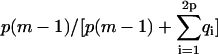 for case C.
Even without a numerical analysis of our model, we can already predict the roles of the free-energy parameters and the way they interact. For the reference interaction free energy, we know that a high value (a low value of k) serves to inhibit intermonomer association, causing monomers to dominate. For high values of k, on the other hand, assembly takes place. We focus here on the latter, more interesting case, and look at two regimes, one where the Boltzmann weight of the lateral-binding free energy, f, is very small, and one where it is not.
In the former regime, a small value of s results in the formation of monomers, dimers, and non-β-type filaments as the dominant species. Conversely, large values of s favor the formation of filaments with a high β-sheet content. The role of the parameter σ, connected to the formation of interfaces between ordered and disordered regions along the chain, now depends on the boundary conditions. If the boundary conditions prescribe disordered ends and s is small, or if the boundary conditions prescribe ordered ends and s is large, the value of σ has little effect, as few interfaces shall form. However, if the boundary conditions prescribe a state that is unfavorable, given the value of s, then interfaces must form in any long filaments or fibrils. If such interfaces carry a large free-energy penalty (i.e., for small values of σ), the aggregates tend to become very long to minimize the number of interfaces by minimizing the number of filaments (28,29,35). For high values of σ, on the other hand, there is little effect.
For high values of f, we expect the fibrillar state to dominate, especially if s is also high. The parameters f and s (and k) are coupled, because each increase in length of the fibrils involves the formation of associations both in the lateral and in the axial direction of the fibril. The importance of the parameter σ depends again on which boundary conditions we impose. In cases B and C, we expect its value to play a small role for high values of s; in case A, however, we again predict a strong increase in the mean fibril length for small values of σ, for the same reasons as those given above for filaments.
We determine the overall properties of the solution of assembling protein molecules by solving z from Eq. 23, for given values of s, f, k, p, σ, and φ, and subsequently inserting the value of z into Eqs. 19, 27, and 32. Because Eq. 23 is a higher-order equation in z, however, we obtain several possible values for z as solutions. As it turns out, in all investigated cases, only one of the solutions is physically relevant. Because z is defined as being an exponential, we can immediately discard any solutions below zero, as well as any imaginary ones. We can test the remaining solutions by inserting them into the equations and calculating the mean lengths and fractions of each aggregated state. For all but one solution, this leads to physically unrealistic values for at least one of these quantities (such as a negative volume fraction, or an aggregate length below unity). The remaining solution is the one we apply (this turns out, in all cases investigated, to be the solution with the lowest value, larger than zero). In the next section, we show our results for different values of the free-energy parameters, for different boundary conditions, and for fibrils containing different numbers of filaments. We focus on the mean degree of polymerization, the mean fibril length, and the weight fractions of the various assembled species.
RESULTS
Boundary conditions
As discussed in the previous section, it is necessary in our model to define a conformation for the ends of the filaments that comprise the fibril. The effect of a change in the description of these ends can be seen in Fig. 3, for the case where we only allow fibrils consisting of two filaments. The mean length of the fibrils is strongly affected by our choice of boundary condition, a result that was also found for aggregates that form by linear self-assembly with a helical transition (29). In amyloid fibrils, for the same values of the free-energy parameters, we observe a much stronger increase in the mean size for the case where each fibril can only have non-β ends than for the other two cases. This is due to the presence of penalized “interfaces” between β-regions and non-β-regions at each of the fibril ends. Because these interfaces are unfavorable, the system strives to minimize their number by allowing fewer (and hence longer) aggregates to form. For the case of thicker fibrils (containing 2–6 filaments), the trends are quite similar (results not shown).
FIGURE 3.

Mean length of fibrils consisting of two filaments as a function of concentration, for s ≡ exp −P = 70, k ≡ exp −M = 50, σ ≡ exp −2R = 0.1, and f ≡ exp −F = 3, and three boundary conditions, as indicated. Case A corresponds to a description in which all fibril ends are fixed to be disordered, case B is that in which they are restricted to a β-strand conformation, and in case C the ends are unrestricted.
In the following we shall determine the impact of the various free-energy parameters, and of the overall protein concentration. First we briefly summarize results of the case where no fibril formation occurs and only monomers, dimers, and filaments are allowed. We then show the case where the only fibrils allowed are those containing two filaments (p = 2). This allows for faster calculations than the case where we allow thicker fibrils, and, as we shall show below, the trends are similar to that case. After this we discuss the more general case where fibrils of two, three, four, five, or six filaments are considered (p = 2–6).
The case where no fibrils form
This case corresponds to a description of linear self-assembly with a conformational transition. Our model to describe this is identical to a recent model for helical self-assembly, and hence our results are also identical (with the β-strand state in this article corresponding to the helical one in earlier works). A full discussion is beyond the scope of this article, and we refer to the earlier work (28,29,35). Summarizing, it was found that the conformational transition can be quite sharp and that it couples to the mean size of the aggregates, resulting in a strong increase in their average degree of polymerization that sets in near the point where the helical conformation becomes dominant.
The case p = 2
Let us now examine the case where the only fibrils that are present consist of two filaments. To study the properties of a solution of this type, we solve Eq. 23 for fixed p = 2, removing the summation in this equation. In the following we focus on the boundary conditions set C (ends are not restricted), but we shall highlight significant differences between the results for different boundary conditions throughout the section. We choose end description C because we (and others) speculate that the fibril ends may have a non-β conformation (4), due to the greater configurational freedom this would allow for these ends. We eliminate case A (which restricts the ends to a non-β conformation) because this leads to extremely large fibril lengths, as seen in Fig. 3. It is, however, not unthinkable that there exist proteins for which the boundary condition A is appropriate.
In Fig. 3, we see that the fibrils are very short at low concentrations, and that they exhibit a strong increase in length at a critical volume fraction of protein molecules (in this case, approximately φ = 2 × 10⁻⁴). (The molar concentration can be determined from the volume fraction φ by dividing the volume fraction by the molecular volume of the protein.) At higher concentrations, the dependence of the mean fibril length (plotted logarithmically) on the logarithm of the volume fraction is linear with a slope of one-half, indicating that, at these concentrations, the mean length of the fibrils scales with the square root of φ. This is the same dependence that is encountered in self-assembled chains (33,35). In this figure and all following ones, we have used for the free-energy parameters values between zero and a few times the thermal energy. Although we do not know exact values for the binding energies between proteins, we estimate that the values we use here are reasonable for monomers that are bonded through nonpermanent, physical interactions. We vary these parameters somewhat between figures, to emphasize the salient features of the fibril formation.
Like the mean size of the fibrils, the composition of the solution also shows a strong dependence on the protein concentration. This is shown in Fig. 4, where we plot the weight fraction of each aggregated species as a function of the volume fraction of protein molecules. As mentioned above, the weight fractions are given by the volume fraction of protein molecules present in a certain state (e.g., monomeric or fibrillar), divided by the total volume fraction of protein molecules, φ. So, for instance, the weight fraction of fibrils is found by dividing Eqs. 26 and 23, for p = 2. The results show that there is a transition between a regime where monomers dominate (at low volume fraction), and one where fibrils dominate, at high volume fraction. (This is true for all three boundary conditions.) This transition can be quite sharp, dependent on the values we choose for the free-energy parameters. The dimers and filaments that are present at low concentrations, are repressed past the transition point, where fibrils dominate. Although it is not immediately clear from this figure, for most of the investigated parameter values, monomers are actually the most abundant species, even at high volume fractions. However, because fibrils can become quite long, the weight fraction of the monomers tends to become negligible when fibrils emerge.
FIGURE 4.

Weight fraction of monomers, dimers, filaments, and fibrils (containing two filaments) in solution, as indicated, as a function of concentration, for s = 10, k = 250, σ = 0.1, and f = 2. (Inset) Same as Fig. 4, but as a function of reference association free energy M, at volume fraction φ = 10−3.
The dependence of the weight fractions on φ, seen in Fig. 4, is reproduced almost exactly in their dependence on the (reference) free energy of a monomer-monomer interaction M, albeit mirrored, as shown in the inset to Fig. 4. This implies that, in the context of our model, the same change in properties may be achieved by a change in the concentration or by a change in the solvent conditions leading to a shift in M.
The mean fraction of material in a β-strand conformation (not shown) is predictably small at low volume fractions (because monomers and dimers, which are defined as disordered, dominate here) and undergoes a sharp transition at the critical concentration to reach values close to unity, following the curve for the weight fraction of fibrils almost exactly (as would be expected for boundary conditions B, where fibrils contain no disordered interactions). This indicates that any disordered ends in the fibrillar state play a small role, either due to the large fibril length or to the circumstance that their presence requires an unfavorable interface to be formed. For values of the free-energy parameters that allow the filament state to play a more prominent role (such as unfavorable values of F) the curve may deviate from the fibril fraction curve, but we still expect a rather sharp transition, the sharper the larger R (28,29,34,35).
The effect of a change in the excess β-association energy, P, can be seen in Fig. 5. Here, too, there are two regimes, one in which fibrils dominate and one in which this is not so. For the same values of the free-energy parameters R and F and the concentration as in the inset to Fig. 4, we find that a decrease of 5 kBT in P suffices to go from a weight fraction of fibrils of approximately zero to one of almost unity. The same is observed in the inset to Fig. 4, for the reference association free energy, M. In fact, the main difference between the insets to Figs. 4 and 5 is the composition of the solution at high values of the free energy. In Fig. 4, monomers dominate, whereas here, there is a significant (and constant) fraction of filaments and dimers present, even at P = 0. This is because, in our model, dimers are defined as disordered (and hence, their fraction is unaffected by the value of P, but affected by that of the reference association free energy M), and filaments are also likely in a non-β conformation, unless the “frustrated monomer” free energy R is small. This means that the fractions of dimers and disordered filaments do not directly depend on the value of P, whereas they must go to zero for high values of M.
FIGURE 5.

Weight fraction of monomers, dimers, filaments, and fibrils (containing two filaments) in solution, as indicated, as a function of excess β-association energy P, for volume fraction φ = 10−3, k = 250, σ = 0.1, and f = 2. (Inset) Mean length of fibrils consisting of two filaments as a function of excess β-association energy P, for the same parameter values as in Fig. 5.
The effect of P on the length of the fibrils, as well as on the overall mean aggregate size (Eq. 27) is shown in the inset to Fig. 5. Here, again, we see the presence of a critical value, above which the increase of the mean aggregate size is slow, and below which the curves are linear. This time the slope of the linear portion of the fibril-length curve equals unity, rather than one-half as was the case with the concentration dependence. We also find that the (free) filaments stay short, regardless of the value of P (not shown). For the cases A and B the trends are the same as in case C, although for case A, the fibril length is much larger than for cases B and C whereas the weight fraction remains the same; see also Fig. 3.
The value of the interface penalty R has no effect on the mean size and solution composition for cases B and C. This is not so for case A, which shows a great increase of the fibril length with increasing R (results not shown). Because in cases B and C the presence of interfaces within the fibrils is either impossible or unlikely for the values of the other energetic parameters used here, the free-energy penalty is not often invoked, and hence has little to no effect. For case A, which is defined as having an interface at every filament end within the fibril, an unfavorable (i.e., large) value of R causes the number of fibrils to decrease, which in turn causes a strong increase in their length. The value of R is known to have a strong effect on the length and conformational state of the filaments as well, and hence we can expect to see the influence of a change in R, even in cases B and C, under circumstances where the filament state dominates (28,34,35).
That the effect of a change in the lateral interfilament binding free energy, F, can be quite drastic (see Fig. 6) is not surprising, given that the linking of two filaments involves a free energy equal to mF with m the length of the filaments. A small change in F then leads to a large change in this free energy. Hence, the system displays a preference for long fibrils for F < 0, expressed by a strong increase of the fibrillization. Nevertheless, we see that the change from a regime where there are hardly any fibrils to one where their weight fraction is almost unity, again requires a change in the relevant free-energy parameter of ∼5 kBT. Filaments, which are the dominant species for high values of F for this set of free-energy parameters, show a very rapid decline as fibrils become dominant. This decrease is also evident in the mean length of the filaments, as shown in the inset to Fig. 6. Contrary to the concentration and the free-energy parameters P and M, the value of F has a relatively modest effect on the mean fibril length in the fibril-rich regime. This is likely due to the circumstance that elongation of (the body of) a fibril requires that at least two monomers become attached to it. This implies an increase of the free energy of F + 2P + 2M. Hence, the effect of a change in F on the length of the fibrils is smaller than those of M and P. The overall mean degree of polymerization, in any case, still shows the same trend as before, a very slow increase, followed by a sudden increase, and a linear dependence of the logarithm of the mean aggregate size on F. The dependence on F follows the same trends for boundary conditions A and B (not shown).
FIGURE 6.

Weight fraction of monomers, dimers, filaments, and fibrils (containing two filaments) in solution, as indicated, as a function of lateral association free energy F, for volume fraction φ = 10−3, k = 250, σ = 0.1, and s = 10. (Inset) Mean length of fibrils consisting of two filaments as a function of lateral association free energy F, for the same parameter values as in Fig. 6.
The case p = 2–6
Let us now generalize our description of fibrils somewhat, and allow fibrils that consist of two, three, four, five, and six filaments to form. For this, we set p0 = 6 in Eqs. 19, 23, and 32. When we compare this to the case where only p = 2 is allowed (see Fig. 7), we see that the sixfold fibrils tend to be much longer than those in the earlier model, but that the trends are the same. The same applies to the mean degree of polymerization. It must be noted, however, that the slopes in the fibril-dominated regime are not all the same. The slope of the curve describing  changes from a value of 4/5 in the case p = 2 to a value of unity for the case p = 2–6. This increased dependence of the mean aggregation number on the concentration must be due to lateral-association effects, because the length of the chains does not show a similar increase; the slopes for the mean length of the thickest fibril allowed both equal one-half.
FIGURE 7.

Mean length of fibrils and mean degree of polymerization as a function of the volume fraction of protein molecules, for s = 15, k = 8, σ = 0.01, and f = 45, and for fibrils consisting of two filaments, and of two to six filaments, as indicated.
Focusing on the dependence of the mean fibril length on the protein volume fraction, we notice that, although there is a sizeable increase in the mean fibril length for those fibrils that consist of six filaments, a similar increase is not seen for fibrils consisting of less than six filaments (the largest increase is seen for p = 5, and even this is almost negligible; see Fig. 8). This corresponds to what is found experimentally, where fibrils are known to have a well-defined, practically monodisperse, diameter (3). The small size of thinner fibrils is likely caused by the circumstance that a sixfold fibril contains m more interfilament contacts than a fivefold one, and hence benefits more from a favorable value of F. Because this is so for any value of p in our model, we may expect that the thickest allowed fibril shall always dominate over thinner fibrils for favorable values of F. This does not correspond to the observation of an optimum fibril thickness in experimental studies. To quantitatively take this into account, we have to include more detailed structural information in our model (see also below). A study to this effect is currently in progress.
FIGURE 8.

Mean length of fibrils consisting of five and six filaments and overall mean degree of polymerization as a function of the protein volume fraction, for s = 15, k = 8, σ = 0.01, and f = 45.
Let us now examine the weight fraction of the aggregated states as a function of protein volume fraction and M. Again the two plots (Fig. 9 and its inset) look identical, albeit mirrored, and again we see that there are two regimes, one where fibrils dominate and one where they do not. (The fractions of dimers, filaments, and fibrils with p < 6 are indistinguishable from zero in the plot and hence are omitted.) The transition is, however, far less gradual than was the case for p = 2, and the change in the slope of the curve is very sudden. This is probably due to the cooperativity in the fibril formation, which is stronger for p = 6 than it is for p = 2, because many more lateral associations are formed in the former case. Similar sharp transitions were observed by Nyrkova and co-workers in their model (11). This is not surprising because our description of the fibrils and theirs closely resemble each other. (Due to the different definitions of the free-energy parameters, a direct comparison of the model of Nyrkova et al. (11) and our model is not possible. We may, however, note that the trends, especially in the fibril-dominated regime, of our model and theirs, are similar.)
FIGURE 9.

Weight fraction of monomers and fibrils (containing two to six filaments) in solution, as indicated, as a function of protein volume fraction, for s = 15, k = 8, σ = 0.01, and f = 45. (Inset) Same as Fig. 9, but as a function of association free energy M, at volume fraction φ = 10−3.
Contrary to our model, Nyrkova's model presupposes a β-sheet structure for all assemblies, with the exception of the monomers. Note that in the limit where the (ordered) fibrils dominate, the fraction of any disordered assemblies is likely very small; the Nyrkova model may provide a very good description when this is the case. Therefore, it may be used pragmatically even in cases where disordered aggregates are known to form. The circumstance that the Nyrkova model essentially uses three parameters, rather than our four, makes it a very attractive model in this regard. Nonetheless, there most likely exist fibril-forming proteins that require disordered protein aggregates to be taken into account explicitly. Indeed, several studies have indicated that (partially) disordered protein molecules may play an important role in the fibrillogenesis (4,6,19,21,23).
As already advertised in the Theory section, we now study what the effect of the introduction of an extra parameter f is. This extra parameter would serve to close the cylinder, so that our description corresponds to a fibrillar state, rather than a sheet-like one. We treat the fibrils with p = 2 as having m lateral interactions, whereas for the larger fibrils we include an extra contact to form the cylindrical fibril. This relatively small change causes a great shift in the size distribution, as the fibrils consisting of three filaments now dominate at high concentrations, both in terms of length and of weight fraction. This shift deserves further study. We speculate that the free energy for ring closure must be unequal to F for systems where thick fibrils are known to dominate, as we argued above. To take the ring closure effect into account in a proper way, it may be necessary to include a p-dependent elastic term in our description of the fibril formation, and to explicitly take into account factors like the architecture of the filaments inside the fibrils, their distribution of hydrophilic and hydrophobic groups, and their helical twist. Some of these effects have been taken into account in Nyrkova et al. (11,40). This shall be explored in a separate publication, in which we compare theory and experiment.
CONCLUSIONS AND OUTLOOK
We have outlined a theoretical treatment for self-assembly with a conformational transition, coupled to the lateral association of chains. Our theory, which is analytical and exact within the model assumptions, mimics the general properties of amyloid fibril formation, in a more detailed manner than has been attempted before. It predicts the mean length of fibrils and the fractions of each aggregated species in dilute solution, as well as the fraction of protein molecules in a β-strand conformation. We find two regimes as a function of concentration and of the free energies of the various types of association: one where fibrils dominate and one where low-molecular-weight species do. The transition between these regimes can be quite sharp because the fibril formation may be highly cooperative. We find that the formation of thick fibrils is favored, and that the fraction of fibrils consisting of fewer than the maximum allowed number of filaments is negligible. The mean fibril length increases slowly at low protein volume fraction, then displays a strong and sharp increase at a critical volume fraction, and then shows a (weaker) exponential increase at higher volume fractions. Similar trends are observed for the mean fibril length as a function of the various association free energies. Finally, we find that our description of the fibril ends can have a large effect on the properties of the aggregates. This effect of boundary conditions seems to indicate that if we can affect the state of the fibril ends, it may prove possible to inhibit the fibril formation.
Our theory is potentially useful in describing the aggregation behavior of any protein that self-assembles into fibrillar structures. Systems that form amyloid fibrils in a way that resembles that of Fig. 1 include certain prion proteins, amyloid β-protein, β-lactoglobulin, τ-protein, insulin, β-microglobulin, α-synuclein, hen egg white lysozyme, and light-chain immunoglobulin. Our model may therefore be useful in their description (4,24,41–46). Although we have focused in the above on amyloidosis, we speculate that the different aggregated states of actin and tubulin (in the presence of abundant GTP) are also reminiscent of those we outline in Fig. 1 (26,27,47,48). In both cases, two conformations are possible (in the case of actin, nonhelical and helical, and in the case of tubulin the so-called straight conformation and the bent one), and in both cases it seems that fibrils can be thought to consist of several laterally associated linear chains.
Note that in the description outlined in the Theory section, we assume that all the steps of the protein fibril formation are reversible. Although this is certainly so for certain proteins, it need not be true for others. Indeed, it is believed that transient species, i.e., thermodynamically unstable aggregates that are rapidly and irreversibly converted into other species, may play a role of some importance in amyloid fibril formation. An example of this type of aggregate is the nucleus that forms and then grows into (the beginnings of) a fibril. Our theory, being statistical-mechanical in origin, cannot in principle describe truly irreversible processes; to provide an accurate description of transient species, a kinetic model is required. Note, however, that by choosing proper values for the free-energy parameters, it is possible to shift the equilibrium between two states to such a degree that the less favorable state becomes negligibly populated.
Because the identity of the nucleus (its size and conformation) and any other unstable species may differ from protein to protein, we have not taken these into account in our general treatment. If one wishes to apply our statistical-mechanical treatment to an experimental system in which aggregates that disappear from the solution in a truly irreversible fashion play a role, one needs to carefully distinguish between the stable states and the transient ones, and only take the former into account. This ensures that the concentration of any unstable intermediate equals zero in equilibrium, whereas stable structures are taken into account in a proper way.
To conclusively determine which systems can be described by the theory as outlined in this article, a detailed comparison between experiment and theory must be performed. This is currently in progress, and shall be discussed in a separate publication. Although the majority of experimental data on amyloid fibril formation is kinetic in nature (i.e., measured as a function of time) there have been some studies of the (equilibrium) fibril length and fibril fraction as a function of concentration (14,17,19). The former type of information may be found from radiation scattering experiments (9,14,17,19,31), whereas the latter type can be obtained by chromatography and sedimentation studies (17,31). There have also been numerous studies that determine the β-sheet content by measuring the fluorescence of the fibrils after thioflavin-T or Congo red binding (18,30), but these techniques seem to be more qualitative than quantitative in nature, as the binding between the dye and the amyloid fibril is still not completely understood. Alternative methods for measuring the fraction of protein in any one conformation may also prove useful in comparing theory and experiment; here one can think of, e.g., circular dichroism spectroscopy (9,10). In addition to concentration dependence, we may look at the temperature dependence of the fibril formation. Although a recent article indicates that this effect is quite small (at large timescales, when the solution has had time to equilibrate) for Aβ peptide (15), this need not be the case for other proteins.
Acknowledgments
The authors are grateful to Jaap Jongejan, Jon Laman, and Maarten Wolf for stimulating discussions.
The authors thank the Netherlands Organization for Scientific Research NWO for funding (grant No. 635.100.012, program for computational life sciences). The authors declare that they have no conflicting financial interests with regards to the publication of this manuscript.
References
- 1.Thirumalai, D., D. K. Klimov, and R. I. Dima. 2003. Emerging ideas on the molecular basis of protein and peptide aggregation. Curr. Opin. Struct. Biol. 13:146–159. [DOI] [PubMed] [Google Scholar]
- 2.Selkoe, D. J. 2002. Deciphering the genesis and fate of amyloid β-protein yields novel therapies for Alzheimer disease. J. Clin. Invest. 110:1375–1381. [DOI] [PMC free article] [PubMed] [Google Scholar]
- 3.Serpell, L. C. 2000. Alzheimer's amyloid fibrils: structure and assembly. Biochim. Biophys. Acta. 1502:16–30. [DOI] [PubMed] [Google Scholar]
- 4.Rochet, J. C., and P. T. Lansbury. 2000. Amyloid fibrillogenesis: themes and variations. Curr. Opin. Struct. Biol. 10:60–68. [DOI] [PubMed] [Google Scholar]
- 5.Petkova, A. T., Y. Ishii, J. J. Balbach, O. N. Antzutkin, R. D. Leapman, F. Delaglio, and R. Tycko. 2002. A structural model for Alzheimer's β-amyloid fibrils based on experimental constraints from solid state NMR. Proc. Natl. Acad. Sci. USA. 99:16742–16747. [DOI] [PMC free article] [PubMed] [Google Scholar]
- 6.Nguyen, H. D., and C. K. Hall. 2004. Molecular dynamics simulations of spontaneous fibril formation by random-coil peptides. Proc. Natl. Acad. Sci. USA. 101:16180–16185. [DOI] [PMC free article] [PubMed] [Google Scholar]
- 7.Collins, S. R., A. Douglass, R. D. Vale, and J. S. Weissman. 2004. Mechanism of prion propagation: amyloid growth occurs by monomer addition. PLoS Biol. 2:1582–1590. [DOI] [PMC free article] [PubMed] [Google Scholar]
- 8.Guo, J. T., R. Wetzel, and X. Ying. 2004. Molecular modeling of the core of Aβ amyloid fibrils. Proteins. 57:357–364. [DOI] [PubMed] [Google Scholar]
- 9.Modler, A. J., K. Gast, G. Lutsch, and G. Damaschun. 2003. Assembly of amyloid protofibrils via critical oligomers: a novel pathway of amyloid formation. J. Mol. Biol. 325:135–148. [DOI] [PubMed] [Google Scholar]
- 10.Kirkitadze, M. D., M. M. Condron, and D. B. Teplow. 2001. Identification and characterization of key kinetic intermediates in amyloid β-protein fibrillogenesis. J. Mol. Biol. 312:1103–1119. [DOI] [PubMed] [Google Scholar]
- 11.Nyrkova, I. A., A. N. Semenov, A. Aggeli, M. Bell, N. Boden, and T. C. B. McLeish. 2000. Self-assembly and structure transformations in living polymers forming fibrils. Eur. Phys. J. B. 17:499–513. [Google Scholar]
- 12.Waterhouse, S. H., and J. A. Gerrard. 2004. Amyloid fibrils in bionanotechnology. Aust. J. Chem. 57:519–523. [Google Scholar]
- 13.Goodsell, D. A. 2004. Bionanotechnology: Lessons from Nature. Wiley-Liss, Hoboken, NJ.
- 14.Lomakin, A., D. S. Chung, G. B. Benedek, D. A. Kirschner, and D. B. Teplow. 1996. On the nucleation and growth of amyloid β-protein fibrils: detection of nuclei and quantitation of rate constants. Proc. Natl. Acad. Sci. USA. 93:1125–1129. [DOI] [PMC free article] [PubMed] [Google Scholar]
- 15.Kusumoto, Y., A. Lomakin, D. B. Teplow, and G. B. Benedek. 1998. Temperature dependence of amyloid β-protein fibrillization. Proc. Natl. Acad. Sci. USA. 95:12277–12282. [DOI] [PMC free article] [PubMed] [Google Scholar]
- 16.Rogers, S. S., P. Venema, L. M. C. Sagis, E. van der Linden, and A. M. Donald. 2005. Measuring the length distribution of a fibril system: a flow birefringence technique applied to amyloid fibrils. Macromolecules. 38:2948–2958. [Google Scholar]
- 17.Walsh, D. M., A. Lomakin, G. B. Benedek, M. M. Condron, and D. B. Teplow. 1997. Amyloid β-protein fibrillogenesis: detection of a protofibrillar intermediate. J. Biol. Chem. 272:22364–22372. [DOI] [PubMed] [Google Scholar]
- 18.Walsh, D. M., D. M. Hartley, Y. Kusumoto, Y. Fezoui, M. M. Condron, A. Lomakin, G. B. Benedek, D. J. Selkoe, and D. B. Teplow. 1999. Amyloid β-protein fibrillogenesis: structure and biological activity of protofibrillar intermediates. J. Biol. Chem. 274:25945–25952. [DOI] [PubMed] [Google Scholar]
- 19.Yong, W., A. Lomakin, M. D. Kirkitadze, D. B. Teplow, S. H. Chen, and G. B. Benedek. 2002. Structure determination of micelle-like intermediates in amyloid β-protein fibril assembly by using small angle neutron scattering. Proc. Natl. Acad. Sci. USA. 99:150–154. [DOI] [PMC free article] [PubMed] [Google Scholar]
- 20.Serpell, L. C., C. C. F. Blake, and P. E. Fraser. 2000. Molecular structure of a fibrillar Alzheimer's Aβ fragment. Biochemistry. 39:13269–13275. [DOI] [PubMed] [Google Scholar]
- 21.Harper, J. D., S. S. Wong, C. M. Lieber, and P. T. Lansbury. 1999. Assembly of A beta amyloid protofibrils: an in vitro model for a possible early event in Alzheimer's disease. Biochemistry. 38:8972–8980. [DOI] [PubMed] [Google Scholar]
- 22.Straub, J. E., J. Guevara, S. H. Huo, and J. P. Lee. 2002. Long time dynamic simulations: exploring the folding pathways of an Alzheimer's amyloid Aβ-peptide. Acc. Chem. Res. 35:473–481. [DOI] [PubMed] [Google Scholar]
- 23.Ma, B. Y., and R. Nussinov. 2002. Molecular dynamics simulations of alanine rich β-sheet oligomers: insight into amyloid formation. Protein Sci. 11:2335–2350. [DOI] [PMC free article] [PubMed] [Google Scholar]
- 24.Khurana, R., C. Ionescu-Zanetti, M. Pope, J. Li, L. Nielson, M. Ramirez-Alvarado, L. Regan, A. L. Fink, and S. A. Carter. 2003. A general model for amyloid fibril assembly based on morphological studies using atomic force microscopy. Biophys. J. 85:1135–1144. [DOI] [PMC free article] [PubMed] [Google Scholar]
- 25.Inouye, H., and D. A. Kirschner. 2000. Aβ fibrillogenesis: kinetic parameters for fibril formation from Congo red binding. J. Struct. Biol. 130:123–129. [DOI] [PubMed] [Google Scholar]
- 26.Oosawa, F., and M. Kasai. 1962. Theory of linear and helical aggregations of macromolecules. J. Mol. Biol. 4:10–21. [DOI] [PubMed] [Google Scholar]
- 27.Oosawa, F., and S. Asakura. 1975. Thermodynamics of the Polymerization of Protein. Academic Press, New York.
- 28.van Gestel, J., P. van der Schoot, and M. A. J. Michels. 2001. Helical transition of polymer-like assemblies in solution. J. Phys. Chem. B. 105:10691–10699. [Google Scholar]
- 29.van Gestel, J., P. van der Schoot, and M. A. J. Michels. 2003. Role of end effects in helical aggregation. Langmuir. 19:1375–1383. [Google Scholar]
- 30.Hasegawa, K., I. Yamaguchi, S. Omata, F. Gejyo, and H. Naiki. 1999. Interaction between Aβ(1–42) and Aβ(1–40) in Alzheimer's β-amyloid fibril formation in vitro. Biochemistry. 38:15514–15521. [DOI] [PubMed] [Google Scholar]
- 31.Pallitto, M. M., and R. M. Murphy. 2001. A mathematical model of the kinetics of β-amyloid fibril growth from the denatured state. Biophys. J. 81:1805–1822. [DOI] [PMC free article] [PubMed] [Google Scholar]
- 32.Reference deleted in proof.
- 33.Cates, M. E., and S. J. Candau. 1990. Statics and dynamics of worm-like surfactant micelles. J. Phys. Cond. Matt. 2:6869–6892. [Google Scholar]
- 34.Zimm, B. H., and J. K. Bragg. 1959. Theory of the phase transition between helix and random coil in polypeptide chains. J. Chem. Phys. 31:526–535. [Google Scholar]
- 35.van der Schoot, P., M. A. J. Michels, L. Brunsveld, R. P. Sijbesma, and A. Ramzi. 2000. Helical transition and growth of supramolecular assemblies of chiral discotic molecules. Langmuir. 16:10076–10083. [Google Scholar]
- 36.Poland, D., and H. A. Scheraga. 1970. Theory of Helix-Coil Transition in Biopolymers. Academic Press, New York.
- 37.Reference deleted in proof.
- 38.Reference deleted in proof.
- 39.Reference deleted in proof.
- 40.Nyrkova, I. A., A. N. Semenov, A. Aggeli, and N. Boden. 2000. Fibril stability in solutions of twisted β-sheet peptides: a new kind of micellization in chiral systems. Eur. Phys. J. B. 17:481–497. [Google Scholar]
- 41.Krishnan, R., and S. L. Lindquist. 2005. Structural insights into a yeast prion illuminate nucleation and strain diversity. Nature. 435:765–772. [DOI] [PMC free article] [PubMed] [Google Scholar]
- 42.McParland, V. J., N. M. Kad, A. P. Kalverda, A. Brown, P. Kirwin-Jones, M. G. Hunter, M. Sunde, and S. E. Radford. 2000. Partially unfolded states of β2-microglobulin and amyloid formation in vitro. Biochemistry. 39:8735–8746. [DOI] [PubMed] [Google Scholar]
- 43.Friedhoff, P., M. von Bergen, E.-M. Mandelkow, P. Davies, and E. Mandelkow. 1998. A nucleated assembly mechanism of Alzheimer paired helical filaments. Proc. Natl. Acad. Sci. USA. 95:15712–15717. [DOI] [PMC free article] [PubMed] [Google Scholar]
- 44.Cao, A., D. Hu, and L. Lai. 2004. Formation of amyloid fibrils from fully reduced hen egg white lysozyme. Protein Sci. 13:319–324. [DOI] [PMC free article] [PubMed] [Google Scholar]
- 45.Souillac, P. O., V. N. Uversky, I. S. Millett, R. Khurana, S. Doniach, and A. L. Fink. 2002. Effect of association state and conformational stability on the kinetics of immunoglobulin light chain amyloid fibril formation at physiological pH. J. Biol. Chem. 277:12657–12665. [DOI] [PubMed] [Google Scholar]
- 46.Hamada, D., and C. M. Dobson. 2002. A kinetic study of β-lactoglobulin amyloid fibril formation promoted by urea. Protein Sci. 11:2417–2426. [DOI] [PMC free article] [PubMed] [Google Scholar]
- 47.Inclán, Y. F., and E. Nogales. 2000. Structural models for the self-assembly and microtubule interactions of γ-, δ- and ɛ-tubulin. J. Cell Sci. 114:413–422. [DOI] [PubMed] [Google Scholar]
- 48.Aldaz, H., L. M. Rice, T. Stearns, and D. A. Agard. 2005. Insights into microtubule nucleation from the crystal structure of human γ-tubulin. Nature. 435:523–527. [DOI] [PubMed] [Google Scholar]