On the Meaning and Existence of an Effective Population Size

Abstract

We investigate conditions under which a model with stochastic demography or population structure converges to the coalescent with a linear change in timescale. We argue that this is a necessary condition for the existence of a meaningful effective population size. We find that such a linear timescale change is obtained when demographic fluctuations and coalescence events occur on different timescales. Simple models of population structure and randomly fluctuating population size are used to exemplify the ideas and provide an intuitive feel for the meaning of the conditions.

IN population genetics, simplifying assumptions are necessary to turn complex biological systems into caricatures that are, on the one hand, simple enough to analyze and, on the other hand, realistic enough to capture key features of the process under investigation. These simple models often make assumptions that are clearly violated in most populations; yet they are of great importance since their simplicity allows one to make predictions about the patterns of polymorphism that are expected under these assumptions. Data can then be compared with these predictions to detect deviations from the simplifying assumptions. In other words, these simple models serve as null models. The standard population genetic null model, the Wright-Fisher model, and its retrospective cousin, the standard coalescent, are examples of this.

The concept of effective population size has traditionally been used to rescale a given population model so that it behaves, with regard to certain properties, as a simple Wright-Fisher model with constant population size. The three properties of the Wright-Fisher model most commonly used in defining effective population sizes are: (i) the probability of identity-by-descent of two alleles chosen at random, (ii) the variance in offspring allele frequency, and (iii) the leading non-unit eigenvalue of the allele frequency transition matrix. They correspond, respectively, to the “inbreeding effective population size,” the “variance effective population size,” and the “eigenvalue effective population size.” In some demographic models the three effective sizes are equal but in others they can differ considerably or simply not exist (Ewens 1982; Orive 1993). Even when they can be defined, they may lead to complex formulas involving demographic parameters that are practically impossible to measure. Furthermore, one too often reads of “the” effective population size without reference to the particular notion being considered.

We propose that the coalescent effective population size introduced and discussed in Nordborg and Krone (2002), when it exists, provides a more general and consistent notion of effective size that is less likely to be misused. Since the coalescent essentially embodies all of the information that can be found in sampled genetic data, one can argue that, if anything deserves the title of “the effective size,” it is the coalescent effective size.

By definition, the coalescent effective size exists only when the scaling of time to retrieve the standard coalescent is independent of time; but, when this is the case, the appropriately rescaled population behaves precisely as the Wright-Fisher model does in all respects. Likewise, when it does not exist, the Wright-Fisher model can be rejected as a null model. As already pointed by Nordborg and Krone (2002) the nonexistence of an effective population size in some situations is a desirable property, at least if the purpose of defining an effective population size is to investigate how genetic drift operates, because it stresses that these situations cannot be described by a Wright-Fisher model.

The Wright-Fisher null model has proved surprisingly difficult to reject, despite what appear to be major violations of the assumptions. This is due to the “robustness” of the coalescent process, which is one of three properties listed by Kingman (2000) as fundamental to this process. Even if a natural population does not fulfill all the assumptions of the Wright-Fisher model, it can sometimes behave in all important respects (i.e., those that are observable from a sample and hence derivable from the genealogy) like a Wright-Fisher population. This happens when the ancestral process can be approximated by Kingman's coalescent with the population size replaced by a constant—the coalescent effective population size, N_e. On the positive side, this means that the coalescent process—and thus the Wright-Fisher model—manages to capture something essential about the way natural populations behave; in other words, it is robust to changes in the assumptions and is therefore a good approximation to real systems. More disturbingly, this lack of sensitivity also implies that certain seemingly important features of the population history cannot be detected using polymorphism data.

In this article we assess conditions under which the coalescent effective size exists, both analytically and through computer simulations. In the simulations we use two simple demographic models, one with randomly fluctuating population size and the other with subdivided populations linked by migration.

THE COALESCENT

The coalescent is a random tree that allows one to characterize ancestral relationships between individuals (genes) in a sample when the population size is large (Kingman 1982a,b,c). The probabilistic structure of Kingman's coalescent (sometimes referred to as the standard coalescent) is quite simple. If we start with a sample of n individuals, we wait a random time T_n that is exponentially distributed with mean 1/

n

2

. At this time, two randomly chosen ancestral lineages coalesce, leaving n − 1 distinct lineages. The lineages continue coalescing in this way until we reach a single common ancestor for the sample. We thus obtain a sequence T_n, T_n−1, … , T₂ of intercoalescence times that are independent and exponentially distributed with

where

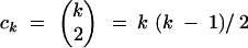is the number of ways to choose an unordered pair from k objects. The time to reach the most recent common ancestor is thus the sum

with expected value

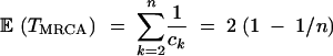Since the standard coalescent corresponds to a neutral Wright-Fisher model, the pairs of lineages that join at coalescence times are always chosen at random. Thus, the probabilistic structure of the coalescent tree is determined by the pure death process that keeps track of the number of ancestral lineages as time recedes into the past.

How Kingman's coalescent relates to the ancestry in a given population genetic model is described most easily for the haploid Wright-Fisher model with fixed population size N and no selection or recombination. In this panmictic model, when N is sufficiently large and time is measured in units of N generations, the ancestry of a sample is approximated by Kingman's coalescent.

Thus to do a calculation for the Wright-Fisher model one does the analogous calculation for the coalescent process and then interprets t units of coalescent time to be [Nt] generations, where [Nt] is the largest integer less than or equal to Nt. For example, the mean time to go from k lineages to k − 1 in the coalescent is E[T_k] = 1/c_k. Thus, in the Wright-Fisher model with population size N, it takes on average N/c_k generations for k lineages to coalesce down to k − 1. With the appropriate scaling of time this approximation works well beyond the Wright-Fisher model and there are variations of the coalescent that incorporate the effects of selection, recombination, spatial structure, and demographic variation.

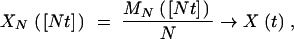
Mathematically, the above can be expressed as follows. Let A(t) denote the number of lineages in the standard coalescent t units of (coalescent) time in the past, and let A_N(τ) be the number of ancestors τ generations in the past for the discrete-time neutral Wright-Fisher model corresponding to fixed population size N. Convergence to the coalescent then means A_N([Nt]) → A(t), as N tends to infinity. If we are dealing with a different population model that has some quantity fluctuating over time, we say “averaging occurs” if the corresponding discrete-time ancestral process satisfies A_N([Nt]) → A(ct) for some constant c. This means that, after converting t units of coalescence time to [Nt] generations, the ancestral process for the discrete-time model can be approximated by the standard coalescent with time speeded up by a factor c. This scaling factor c then allows us to define the coalescent effective population size by

Note that speeding up the coalescent by a factor c is equivalent, as far as sample data are concerned, to multiplying the mutation rate by the factor 1/c. Thus, we get the same genealogy as for a neutral, panmictic, constant-size Wright-Fisher model with a different mutation rate. Indeed, if there is a scaling constant c such that the appropriately scaled ancestral process converges to A(ct), then the sampled data cannot be distinguished from those arising in a standard neutral Wright-Fisher model. Other “coalescent effective population sizes” have been defined in, e.g., Gillespie (2000) and Sano et al. (2004), but both differ from our definition. Gillespie's coalescent effective population size was defined in relation to the presence of hitchhiking but did not explicitly consider other possible departures from the standard Wright-Fisher model. The definition of Sano et al. of coalescent effective population size is closer to ours as it also stems from considering fluctuating population sizes but it does not require a linear scaling of time. In other words, our definition implies that the coalescent N_e of Sano et al. exists but the converse is not true. Note also that the coalescent effective population size proposed here makes sense only when the coalescent approximation applies. In particular this implies that the population size must be much larger than the sample size (Kingman 1982a,b,c). Furthermore, this definition does not allow for an effective population size in models that converge to types of coalescent processes other than the standard coalescent. For instance, there is no effective population size in models that converge to the “structured coalescent” (Notohara 1990; Herbots 1997) or the coalescent process described by Wakeley and Aliacar (2001), where there is an “initial scattering phase” followed by a “collecting phase.”

In this article, we seek to determine when, in the presence of stochastic demography (e.g., fluctuating population size or spatial structure), we can define an effective population size, N_e, that allows us to do all coalescent-based calculations in the same way as we would for a Wright-Fisher model with size N_e. Our approach involves both theoretical analysis and simulations.

Our analytical results will provide general insight into the effects of fluctuating population size and geographical structure on the genealogical process. We will see, for example, that these effects can be averaged to get a coalescent effective size if population size fluctuations and migration rates are sufficiently rapid. To get a feel for how these limiting results apply to real populations and to gauge their robustness, we use simulations. For this, we quantify the effects of deviations from the standard constant-size Wright-Fisher model with Fu and Li's F-statistic (Fu and Li 1993), one of many statistics designed to detect such deviations. We simulated Tajima's D (Tajima 1989) as well but as the result was qualitatively the same; we henceforth deal only with F.

The F-statistic is defined by

where n is the sample size, π is the average number of pairwise nucleotide differences (the average being over all possible pairs in the sample), S is the number of segregating sites, η_s is the number of singletons (mutations that appear in only one individual in the sample), and μ_F and ν_F are constants given the sample size n. This construction yields an expected value that is nearly zero (actually, it is slightly negative), assuming the standard model and the infinitely many sites model, but is expected to deviate from zero when the assumptions are not met. For example, fluctuating size tends to produce negative values of F and population subdivision leads to positive F.

The rest of the article is arranged as follows. In the next section, we discuss the case of randomly fluctuating population size. We begin with a fairly thorough treatment of the analytical results that describe when one can and cannot get a coalescent effective population size. This is followed by simulations of Fu and Li's F for a special case of the model. This section is followed by a more abbreviated one dealing with population structure. Again, we begin with an analytical discussion and follow it with simulations in a special case. A discussion section summarizes the results and in the appendix we show how to get the nonlinear time change for “intermediate” rates of population size fluctuations.

FLUCTUATING POPULATION SIZE

In this section, we discuss the effects of stochastically fluctuating population size on haploid, neutral, single-locus gene genealogies. This differs in a fundamental way from coalescent theory in the presence of deterministically varying population size.

If these size fluctuations are fast compared to the coalescent timescale, then they will affect the coalescent only in an average sense. In this case there will be an effective population size and the genealogy will be given by Kingman's coalescent with a linear time change. If, on the other hand, “macroscopic” size fluctuations occur on the same timescale as coalescences, then the resulting genealogical process will be described by Kingman's coalescent run on a nonlinear, stochastic timescale. In this case, there is no effective population size. The object that one would like to think of as an effective size in this case changes with time instead of being constant; essentially, there is only an “instantaneous” effective size.

Fast fluctuations—averaging:

One often sees in population genetics the claim that, when population sizes fluctuate, there is an effective size given by the harmonic mean of the possible sizes. To understand when this works and, more importantly, when it does not, let us begin with a simple calculation.

Suppose the sizes of a population have some fixed discrete set of possible values, denoted by N₁, N₂, … , and assume that these sizes are all multiples of some large value N, say N_i = x_iN for each i, where the x_i are fixed positive numbers. As is typical in coalescent theory, we think of N as a parameter that gives the magnitude of population size. Denote by M_N(0), M_N(1), M_N(2), … the sequence of population sizes backward in time; i.e., M_N(0) is the size of the current generation, M_N(1) is the size of the previous generation, etc. The simplest possible model of randomly fluctuating size would assume that M_N(0), M_N(1), M_N(2), … form an independent, identically distributed sequence with probabilities p_i ≡ P(M_N(τ) = N_i) for each time τ ≥ 0. Suppose for simplicity that we have a Wright-Fisher model of reproduction, so that the probability of two randomly chosen individuals in generation τ − 1 having a common parent in generation τ is 1/M_N(τ). Then we compute the probability that two individuals do not have a common ancestor [Nt] generations in the past (i.e., their ancestral lineages have not yet coalesced),

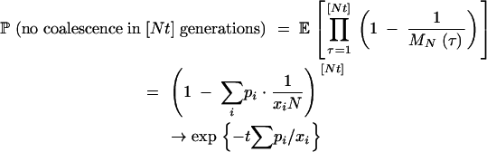as N → ∞. In the first equality, we conditioned on the values of the population sizes and then averaged over all possibilities; in the second equality we used the assumption that sizes were iid to bring the expectation inside the product and turn the product into a power.

This calculation suggests that the pairwise coalescence rate, when N is large, should be given by ∑p_i/x_i. This means that the pairwise coalescence probability in one generation is of the form (1/N)∑p_i/x_i. To match the Wright-Fisher dynamics, this last quantity is set to 1 over the effective population size; i.e., the effective size N_e = (∑p_i/N_i)⁻¹ is given by the harmonic mean of the possible sizes.

The above calculations depend on population size being independent between generations, which is hardly a realistic assumption. However, using the methods in Nordborg and Krone (2002), one can extend this to the case where the sequence (M_N(τ))_τ≥0 is allowed to change every generation according to a discrete-time Markov chain with state space {N₁, N₂, …} and unique stationary distribution (π₁, π₂, …). Then, as in the iid example, the effects of fluctuating size “average” between coalescence events, this time giving an effective pairwise coalescence rate of ∑π_i/x_i and hence an effective size N_e = (∑π_i/N_i)⁻¹, which is again a harmonic mean with the averaging being done with respect to the stationary distribution. Jagers and Sagitov (2004) obtain similar results for general reproduction models and stationary Markovian population size with a finite number of states.

More generally, and using again the methods in Nordborg and Krone (2002), the same conclusion is reached if the size jump probability (per generation) is of the form p_ij = q_ij/N^α, whenever 0 ≤ α < 1. This means that size fluctuations are fast compared to coalescence events.

Slow fluctuations:

Similarly, if the large changes in population size are sufficiently slow compared to coalescence events, then in the limiting (N → ∞) coalescent all the coalescences will occur before there are any changes in size. This means that the limiting coalescent will correspond to a model in which the population size does not change and hence, in a simplistic way, one can think of having an effective size given by the initial size. This situation does not, however, entail averaging.

Intermediate fluctuations—no averaging:

The remaining case, in which “large” changes in population size occur on the same timescale as coalescence events, has been treated mathematically by Kaj and Krone (2003)(see also Donnelly and Kurtz 1999). In this case, there will be no averaging of the effects of size fluctuations, and hence there is no effective population size. Rather, the size fluctuations on this scale directly affect the timescale of the coalescent in a nonlinear, stochastic manner. In other words, the coalescent in this setting is given by a time change of Kingman's coalescent, but now the time change is a random process and not a linear function of t, which is what would happen in the case of averaging.

To make this precise, consider a single haploid population with size M_N(τ), τ generations in the past, and write

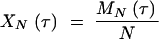1

for the relative size process, where N is a parameter that we take to be large. We assume that this process, when run on the coalescent timescale, converges to a process {X(t) : t ∈ [0, ∞)} with state space I ⊆ (0, ∞),

2

as N → ∞.

We have in mind, primarily, three kinds of limit processes:

• Case i. One-dimensional diffusion: X is a diffusion process with state space given by some interval [a, b], where a > 0.

• Case ii. Jump process: X is a continuous-time Markov jump process with bounded jump intensities and state space I given by a discrete subset of (0, ∞).

• Case iii. Mixture: We can also consider combinations of the above, i.e., diffusion plus occasional large jumps. This includes as a special case deterministic continuous size change (e.g., exponential decay, reflecting exponential growth forward in time) with occasional random jumps.

Note that case i contains as a trivial special case the usual models of deterministic size fluctuations as discussed, for example, in Griffiths and Tavaré (1994). In other words, the diffusion coefficient is zero in such models.

Intuitively, for the diffusion limit to occur, the scaled size process X_N(·) should make frequent (say every generation) small jumps (of order 1/N). For example, if I = [a, b] is the state space for the limiting diffusion, the state space for X_N(·) might be of the form I_N ≡ I ∩ Z_N, where Z_N = (1/N)Z is the set of all integer multiples of 1/N.

A typical example of case ii occurs when the process X_N(·) jumps within a fixed discrete set (possibly finite), and the probability of jumping out of a given state in one generation is of order 1/N. Then, for a given N, the holding time in a given state is geometric with parameter p_N ∼ O(1/N). These geometric holding times converge to exponential holding times as N → ∞. As we mentioned above, the thing to keep in mind in all these cases is that macroscopic changes in population size occur on the same timescale as coalescence events.

We show in the appendix that, in the limiting coalescent, the pairwise coalescence probability during [0, t] is determined by the cumulative coalescence intensity over the time interval [0, t],

where X(t) is the scaled backward size process (Kaj and Krone 2003; Donnelly and Kurtz 1999). Thus, when there are k lineages, the coalescence intensity grows like

k

2

Y_t. In other words, if A(t) is Kingman's coalescent process, the limiting coalescent in the above setting is given by A(Y_t). This is Kingman's coalescent run according to the nonlinear stochastic clock Y_t. This can be envisioned as moving up the standard coalescent tree at a rate that varies according to what the current size is. Note that the initial population size matters, unlike what happens in the case of averaging. This dependence is also seen in the simulations when size fluctuations are sufficiently slow. Time changes of this form have already been noted (Griffiths and Tavaré 1994) in cases for which the past population sizes are assumed known (e.g., a population that is exponentially growing forward in time). The result indicated in this article is much more general and accounts for an important source of randomness in the population size process. In fact, one of our major goals is to provide some guidance on when the speed and intensity of the fluctuations in the size process produce polymorphism data that are not compatible with an equivalent constant-size model.

Simulation results:

We consider a simple model in which the population size has two possible values and falls within the realm of case ii above. This model has been studied by Iizuka and co-workers in the context of inbreeding (Iizuka 2001) and heterozygosity (Iizuka et al. 2002) effective population sizes. Four parameters—two population sizes, N₁ and N₂ (with N₁ < N₂), and two transition probabilities, q₁ and q₂—give the one-step probabilities of size changes from N₁ to N₂ and from N₂ to N₁, respectively. Thus, the size process describing the demographic process is a discrete-time Markov chain with state space {N₁, N₂} and unique stationary distribution π with π(N₁) = q₂/(q₁ + q₂) and π(N₂) = q₁/(q₁ + q₂).

The parameter values used in our simulations were N₂ = 10⁴ and 10⁵, while N₁ was fixed at 10³. For simplicity, we set q₁ = q₂ and values used were 1, 0.75, 0.5, 10^−0.5, 10⁻¹, 10^−1.5, … , 10⁻⁶. The mutation probability per individual per generation was fixed at μ = 0.001. For details about the simulations, see the appendix. Dependence on initial size is one of the hallmarks of the nonaveraging case. It is tempting to think that one might obtain averaging, and hence a linear time change in the coalescent, by starting the demographic process at its stationary distribution. A heuristic argument for why this will not work can be made along the following lines. Because q₁ = q₂, we expect the demographic process to spend as much time in state N₁ as in N₂. However, because N₁ < N₂, the coalescence rate is higher while the population size is N₁. The combined effect is that, conditional on a coalescence event happening in generation τ, the population size of generation τ is more likely to be N₁, implying that the distribution of the demographic variable at τ is no longer given by the stationary distribution with which we started. When the demographic process is much faster than coalescence events, however, we would expect this effect to be negligible and the genealogy to behave as in a constant-size null model.

As predicted, departures from the null model are detected only when the fluctuations in population size are intermediate. The range of q that corresponded to the demographic process being sufficiently intermediate to make rejecting the constant-size null model likely appears to be given by the interval [1/N₂, 1/N₁] extended by 1 order of magnitude on either side, i.e., [10⁻⁵, 10⁻²] for N₂ = 10⁴, N₁ = 10³ and [10⁻⁶, 10⁻²] for N₂ = 10⁵, N₁ = 10³ (Figure 1). For q > 10/N₁, fluctuations are fast enough to give F values that are consistent with a null model with an appropriately averaged constant effective size. For q < 1/(10N₂), the size fluctuations are slow enough to give F values consistent with population size fixed at the initial value.

Figure 1.—

F when N₁ = 10³, μ = 0.001, and q₁ = q₂. Each point represents an average from 10,000 runs starting with the stationary probability of being in N₁. (Top) N₂ = 10⁴; (bottom) N₂ = 10⁵.

Not surprisingly, the extent to which F deviates from zero increases as the difference between N₁ and N₂ increases. As long as population size fluctuations are small, they have little effect.

When size fluctuations do have an effect on F, the effect increases with sample size. This is expected because, as the sample size increases, so does the time to the most recent common ancestor. However, the phenomenon becomes less marked as the sample size gets very large. This is a consequence of the fact that the expected time to the most recent common ancestor reaches a limit as the sample size goes to infinity.

Figure 2 shows that F tended to be more negative when the initial population size was the larger one (N₂). The reason for this is that the coalescence rate is smaller when the population size is N₂ (because N₂ > N₁). Thus, since q₁ = q₂, a population size change before a coalescence event is more likely when the population size is N₂ than N₁.

Figure 2.—

Fu and Li's F, for fluctuating population size, when N₁ = 10³, N₂ = 10⁵, and q₁ = q₂ = 10⁻⁴. The top curve corresponds to initial population size 10³ and the bottom curve to initial population size 10⁵.

STRUCTURED POPULATIONS

In this section, we consider the effects of population subdivision on genealogical processes and discuss under which conditions averaging occurs. In other words, we seek conditions under which one can think of the population as being equivalent to a single panmictic unit with some constant effective size. Here, population subdivision might refer to geographical structure with, for example, fixed-sized demes connected by migration. More generally, it refers to any partitioning of the population into different “types” of individuals, with a corresponding “migration” of types. When appropriately scaled, the resulting ancestral process often converges to a structured coalescent (Notohara 1990; Herbots 1997) in which lineages within a deme can coalesce, as in the coalescent, and lineages occasionally migrate between demes.

Our interest here is in finding conditions under which the limiting genealogy is identical to a standard coalescent relative to a single effective population size. This was discussed at length by Nordborg and Krone (2002), and we refer to that article and the references therein for details. We contend ourselves with a brief summary of the main ideas, followed by simulations for a special case to get a feel for when these approximations work in finite populations.

If migration between subpopulations is sufficiently fast compared to the coalescent timescale, the effects of subdivision will be felt in the coalescent in an average sense only [this is the “strong migration limit” (Nagylaki 1980)]. Essentially, the migration process has time to reach equilibrium between coalescence events.

In this case there will be a coalescent effective population size and the genealogy will be given by Kingman's coalescent with a linear time change. If, on the other hand, migration events are intermediate in the sense that they occur on the same timescale as coalescences, then the resulting genealogical process will be described by a structured coalescent. In this case, the genealogy cannot be thought of a standard coalescent and there is no coalescent effective population size.

To make this more precise, let us consider a scenario in which a population is broken up into a finite number, L, of demes and that the size of deme i is the constant N_i = a_iN, where a₁ + · · · + a_L = 1; hence N is the total population size. Since coalescence probabilities in discrete-time-structured models depend on the locations of the lineages in addition to the total number of lineages, the genealogy is a function of the backward configuration process, X(τ) = (X₁(τ), … , X_L(τ)), where X_i(τ) denotes the number of ancestors in deme i, τ generations into the past. This is a discrete-time Markov chain whose state space consists of vectors x = (x₁, … , x_L), which specify, at any time in the past, the number of ancestral lineages in each deme. The configuration process evolves by (backward) migration and coalescing of ancestors with the appropriate probabilities as we move back in time one generation at a time. In general, coalescence probabilities change when the configuration process changes. Let b_ij denote the probability that a given lineage “migrates” from deme i to deme j one generation back in time. For example, if the forward migration probabilities are denoted by m_ij, then we would have

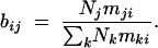3

Suppose that lineages migrate (backward) independently of one other and that the backward migration process determined by the b_ij's is irreducible and aperiodic with stationary distribution γ = (γ₁, γ₂, … , γ_L). Finally, assume that the above backward migration probabilities scale like b_ij = β_ij/N^α, i ≠ j, for some 0 ≤ α ≤ 1. Of course, . In this case, we say that b_ij has scaling exponent α.

Migration probabilities with scaling exponent α correspond to migration events that take, on average, O(N^α) generations to occur. In particular, when 0 ≤ α < 1, migration events occur much faster than coalescence events (when N is large). In this case, Nordborg and Krone (2002) show, under mild conditions, that the ancestral process for the discrete-time model can be approximated by a linear time change of the standard coalescent. The coalescence rate when there are r lineages is given by

Thus, there is a scaling constant

4

that gives the pairwise coalescence rate, and hence the coalescent effective population size is

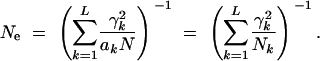5

Note that this can also be thought of as a kind of harmonic mean size in which the weighting factor γ²_k represents the stationary probability of finding two ancestral lineages together in deme k. Thus, when 0 ≤ α < 1, the structured model can be thought of as a panmictic Wright-Fisher model with population size N_e.

When the scaling exponent is α = 1, migration events occur on the same timescale as coalescence events and the stochastic nature of migration does not average out in the limit. In this case, the discrete-time ancestral process converges to a structured coalescent. This maintenance of structure in the limiting genealogy results in, for example, higher variance for sample data than that expected under the standard coalescent; thus we do not expect the same pattern of variation as under the null model.

The above discussion holds in much more generality and we refer the reader to Nordborg and Krone (2002) and references therein for a full discussion. For example, if the scaling exponents are not all the same, all demes connected by fast migration [i.e., scaling exponents in the interval [0, 1)] collapse down to an effectively panmictic group; all migration corresponding to scaling exponent 1 remains in the suitably reduced structured coalescent.

To emphasize the effects of scaling in subdivided populations, we employed the simplest possible model of geographical structure, with two subpopulations of equal size connected by symmetric migration. Two cases of total population size (twice the common subpopulation size), 10³ and 10⁴, were investigated and the scaled migration rate (β = bN, where b is the common migration probability) varied between 10^−1.0 and 10^2.5, the exponent changing in increments of 0.5. The sample was divided equally between the two demes; i.e., half of the lineages started in one subpopulation and the remaining half in the other. As we have seen, an effective size is expected to exist when the migration rate is sufficiently fast.

As shown in Figure 3, F did not differ much from the value that would be expected under a panmictic null model with scaled migration rate 10¹ or larger. This was true for both subpopulation sizes. In other words, F showed the effects of subdivision for b < 10⁻² (resp., b < 10⁻³) when N = 10³ (resp., N = 10⁴) only. Note that the dependence on sample size is prominent only when the migration rate is very small.

Figure 3.—

(Top) F, under the migration model, when the population size is N = 10³; (bottom) N = 10⁴. β = bN, where b is the migration probability.

We emphasize that the flat part of the graph corresponding to fast migration is predicted by the theory. The interesting thing about the simulations is that they point out how fast the migration has to be and show the effects of subdivision on F when migration is not fast enough.

DISCUSSION

We have shown that when demographic processes and coalescence events operate on similar timescales the coalescent effective size does not exist. In other words, the genealogy cannot be expressed by a linear time-scaling of the standard coalescent. As was already pointed out by Nordborg and Krone (2002), the coalescent effective size is conceptually different from classical notions of effective size in that its existence implies that the properly scaled ancestral process converges to Kingman's coalescent with a linear time change. This is a strong condition. Phenomena that can be reduced to an effective population size in our sense are not detectable through polymorphism data alone.

We have shown that convergence to the standard coalescent (with a linear time change) is not always obtained when the population size fluctuates randomly or when the population is subdivided. Whether or not this happens, and hence whether or not there is a coalescent effective size, depends on the relative timescales at which coalescences and demographic processes are operating. This is yet another illustration of the importance of timescales first stressed in Nordborg (1997) and then encapsulated in Möhle's theorem (Möhle 1998). In practice, our simulations suggest that the order of magnitude of the demographic processes should be different from that of the inverse of the population size for the standard coalescent approximation to be sufficiently accurate. By “sufficiently accurate” we mean that deviations from the null model are not expected to be detected in genetic data. To monitor this we used Fu and Li's F and found that, for a simple two-state population-size model, the population size and coalescent processes operate on different timescales when the probability of a state change is not in the range from one order of magnitude less than the inverse of the smaller population size to one order of magnitude more than the inverse of the larger population size. For a simple model of population structure the same is true when the probability of migrating is not higher than the order of magnitude of the inverse of the population size. Thus the results of the two cases are similar; when there is one order of magnitude or more difference between the probability of a demographic change and the probability of a coalescence event, an effective size can be assumed.

APPENDIX

Nonlinear time change for intermediate size fluctuations:

Consider the fluctuating size model discussed in the main text. Let A_N(·) be the ancestral process defined by A_N(0) = n and A_N(τ) = number of distinct ancestors τ generations in the past, τ ≥ 1, where n is the original sample size.

To find the coalescence rate for a pair of lineages, we compute the probability (conditional on population size) that no coalescence has occurred over [Nt] generations and take a limit,

A1

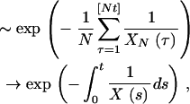A2

as N → ∞. This suggests that, in the limiting coalescent, the coalescence probability for a pair of lineages during [0, t] is governed by an exponential random variable with rate given by ∫^t₀1/Xsds. Thus, as in Griffiths and Tavaré (1994) for deterministic size fluctuations and Kaj and Krone (2003) in the case of stochastic fluctuations, we define the cumulative coalescence intensity over the time interval [0, t] by

This applies to any pair of ancestral lineages, so when there are k lineages, the coalescence intensity grows like

k

2

Y_t. In other words, the limiting coalescent process should be given by

A3

where A(t) is Kingman's coalescent, and Y_t is the increasing, nonlinear stochastic time change. In a more general context, this result was proven in Kaj and Krone (2003) in terms of weak convergence for the bivariate process {(N⁻¹X_N([Nt]), A_N([Nt]))}_t≥0 toward {(X(t), A(Y_t))}_t≥0, as N → ∞.

Relative speed of fluctuations:

Following Sano et al. (2004), we give another perspective on the three time-scaling regimes for the varying size model, now starting from the limit result for the intermediate case and considering two extremes. To this end, let a be a dummy variable signifying a change in speed of the prelimit process from X_N([Nt]) to X_N([aNt]). Then {(N⁻¹X_N([aNt]), A_N([Nt]))}_t≥0 tends toward {(X(at), A(a⁻¹Y_at))}_t≥0 as N → ∞, in agreement with the result quoted above. Here we recognize the regime of slow demographic change by taking a very small. Indeed, as a → 0,

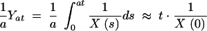so we have linear scaling with effective population size X(0); i.e., on the coalescent timescale, the population size never changes. Similarly, a very large corresponds to the fast scaling regime. In this case, assuming that X(t) is ergodic with a steady state X_∞, the limit a → ∞ gives

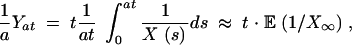which is linear scaling with effective population size given by the harmonic mean 1/E(1/X_∞).

Recall that X(s) represents the (limiting) scaled size process. As is to be expected, the coalescence intensity Y_t increases at a faster rate when X(t) is smaller. Also, during such periods in which Y_t increases faster, there will tend to be fewer mutations. This was brought out in earlier calculations, as well as in the simulations.

The program:

The simulation program, written in C++, can be obtained from the authors upon request. The program simulates the combined effect on F of the ancestral and demographic processes. The models used for the demographic processes were the simplest possible. Fluctuating population size was modeled by a two-state Markov chain and population structure by two equally sized subpopulations with symmetric migration.

Generations were discrete and population sizes finite. For each set of parameters, even sample sizes from 4 to 60 were simulated and the average value of F from 10,000 runs was calculated. The program does not allow for more than two lineages to coalesce at a time. This deviation from the Wright-Fisher model will cause a negative bias in F, but the effect is negligible for the parameter values we used (results not shown; the sample size has to be large relative to the population size for multiple coalescences to the same individual to matter).

Every generation, a gene can mutate with a fixed probability. If no mutations occur in a given realization, F is not defined. One can either define F as zero or disregard these cases. We chose a mutation rate high enough so that our results were unaffected by which method was used.

References

- Donnelly, P., and T. G. Kurtz, 1999. Particle representations for measure-valued population models. Ann. Prob. 27: 166–205. [Google Scholar]
- Ewens, W. J., 1982. The concept of the effective population size. Theor. Popul. Biol. 21: 373–378. [Google Scholar]
- Fu, Y.-X., and W.-H. Li, 1993. Statistical tests of neutrality of mutations. Genetics 133: 693–709. [DOI] [PMC free article] [PubMed] [Google Scholar]
- Gillespie, J. H., 2000. The neutral theory in an infinite population. Gene 261: 11–18. [DOI] [PubMed] [Google Scholar]
- Griffiths, R. C., and S. Tavaré, 1994. Sampling theory for neutral alleles in a varying environment. Philos. Trans. R. Soc. Lond. B Biol. Sci. 344: 403–410. [DOI] [PubMed] [Google Scholar]
- Herbots, H. M., 1997 The structured coalescent, pp. 231–255 in Progress in Population Genetics and Human Evolution, edited by P. Donnelly and S. Tavaré. Springer-Verlag, New York.
- Iizuka, M., 2001. The effective size of fluctuating populations. Theor. Popul. Biol. 59: 281–286. [DOI] [PubMed] [Google Scholar]
- Iizuka, M., H. Tachida and H. Matsuda, 2002. A neutral model with fluctuating population size and its effective size. Genetics 161: 381–388. [DOI] [PMC free article] [PubMed] [Google Scholar]
- Jagers, P., and S. Sagitov, 2004. Convergence to the coalescent in populations of substantially varying size. J. Appl. Prob. 41: 368–378. [Google Scholar]
- Kaj, I., and S. M. Krone, 2003. The coalescent process in a population with stochastically varying size. J. Appl. Prob. 40: 33–48. [Google Scholar]
- Kingman, J. F. C., 1982. a The coalescent. Stoch. Proc. Appl. 13: 235–248. [Google Scholar]
- Kingman, J. F. C., 1982b Exchangeability and the evolution of large populations, pp. 97–112 in Exchangeability in Probability and Statistics, edited by G. Koch and F. Spizzichino. North-Holland Publishing, Amsterdam.
- Kingman, J. F. C., 1982c On the genealogy of large populations, pp. 27–43 in Essays in Statistical Science: Papers in Honour of P. A. P. Moran (J. Appl. Probab., Special Vol. 19A), edited by J. Gani and E. J. Hannan. Applied Probability Trust, Sheffield, England.
- Kingman, J. F. C., 2000. Origins of the coalescent: 1974–1982. Genetics 156: 1461–1463. [DOI] [PMC free article] [PubMed] [Google Scholar]
- Möhle, M., 1998. Robustness results for the coalescent. J. Appl. Probab. 35: 438–447. [Google Scholar]
- Nagylaki, T., 1980. The strong-migration limit in geographically structured populations. J. Math. Biol. 9: 101–114. [DOI] [PubMed] [Google Scholar]
- Nordborg, M., 1997. Structured coalescent processes on different timescales. Genetics 146: 1501–1514. [DOI] [PMC free article] [PubMed] [Google Scholar]
- Nordborg, M., and S. M. Krone, 2002 Separation of time scales and convergence to the coalescent in structured populations, pp. 194–232 in Modern Developments in Theoretical Population Genetics: The Legacy of Gustave Malécot, edited by M. Slatkin and M. Veuille. Oxford University Press, Oxford.
- Notohara, M., 1990. The coalescent and the genealogical process in geographically structured populations. J. Math. Biol. 29: 59–75. [DOI] [PubMed] [Google Scholar]
- Orive, M. E., 1993. Effective population size in organisms with complex life-histories. Theor. Popul. Biol. 44: 316–340. [DOI] [PubMed] [Google Scholar]
- Sano, A., A. Shimizu and M. Iizuka, 2004. Coalescent process with fluctuating population size and its effective size. Theor. Popul. Biol. 65: 39–48. [DOI] [PubMed] [Google Scholar]
- Tajima, F., 1989. Statistical method for testing the neutral mutation hypothesis by DNA polymorphism. Genetics 123: 585–595. [DOI] [PMC free article] [PubMed] [Google Scholar]
- Wakeley, J., and N. Aliacar, 2001. Gene genealogies in a metapopulation. Genetics 159: 893–905. [DOI] [PMC free article] [PubMed] [Google Scholar]