Gaussian-Weighted RMSD Superposition of Proteins: A Structural Comparison for Flexible Proteins and Predicted Protein Structures

Abstract

Many proteins contain flexible structures such as loops and hinged domains. A simple root mean square deviation (RMSD) alignment of two different conformations of the same protein can be skewed by the difference between the mobile regions. To overcome this problem, we have developed a novel method to overlay two protein conformations by their atomic coordinates using a Gaussian-weighted RMSD (wRMSD) fit. The algorithm is based on the Kabsch least-squares method and determines an optimal transformation between two molecules by calculating the minimal weighted deviation between the two coordinate sets. Unlike other techniques that choose subsets of residues to overlay, all atoms are included in the wRMSD overlay. Atoms that barely move between the two conformations will have a greater weighting than those that have a large displacement. Our superposition tool has produced successful alignments when applied to proteins for which two conformations are known. The transformation calculation is heavily weighted by the coordinates of the static region of the two conformations, highlighting the range of flexibility in the overlaid structures. Lastly, we show how wRMSD fits can be used to evaluate predicted protein structures. Comparing a predicted fold to its experimentally determined target structure is another case of comparing two protein conformations of the same sequence, and the degree of alignment directly reflects the quality of the prediction.

INTRODUCTION

Protein flexibility is a common feature of many biological systems that can regulate ligand binding and a large variety of cellular processes. The flexibility of dynamic regions allows a protein to assume multiple conformational states. The conformational change can give rise to motion in molecular motors, act as a switch to turn on or off the respective biological activity, or even allow the same protein to perform several different functions (1–3).

Databases that highlight structural variation through mobility or evolution are useful and growing resources. The Database of Simulated Molecular Motions provides computational data on protein motion and flexibility (4). The Structure Superposition Database was created to address the issue of properly aligning and understanding large sets of homologous protein structures (5). The Database of Macromolecular Movements presents a diverse set of proteins that display large conformational changes in different crystallographic structures (6–8). A recent review discusses a range of motions observed in biopolymer synthesis and membrane transport seen in the Database of Macromolecular Movements (9). For instance, T7 RNA polymerase exhibits a large conformational change from the initiation to elongation phase, and a substantial motion is observed in Ca²⁺-ATPase as it converts between a calcium-bound and free state.

Conformational changes are also observed in protein-protein interactions, which are required in signaling pathways to transmit a message from the extracellular environment to the interior of a cell (10,11). Signaling proteins can communicate through the same interaction domain with many different effectors. This requires that the interaction domain be flexible enough to accommodate structures of various sizes and chemical composition, yet the protein-protein interactions must be specific and selective enough to continue the signal flow.

Freire and co-workers probed the inhomogeneous distribution of stability throughout a protein structure, using an ensemble of conformations (12,13). They concluded that protein binding sites are generally typified by having concomitant regions of low and high structural stability. Flexible regions allow ligands to enter and leave the binding site, and plasticity is required in any induced-fit binding, whether it is a simple side-chain reorientation or movement of a whole domain (2,14). However, the regions of the protein with high structural stability, or “core regions”, remain relatively static between the multiple conformations, despite any movement of the flexible regions.

The heart of comparing two conformations of a flexible protein is an appropriate overlay of the structures for visual inspection. Over a dozen different techniques have been proposed for comparing and overlaying flexible proteins (7,15–27). For almost 20 years, every technique has been based on two steps: first, identify related subsets of Cα in the protein conformations and second, overlay that subset by a standard root mean square deviation (sRMSD) fit. Each technique differs in the way that it identifies the subsets, usually defining static, core regions of the protein. Some methods are quite elegant, even using weighted analytical techniques to define the subsets. The merits and caveats of each technique's definition of a subset are often debated, but when an alignment is made in the end, all of these techniques get simplified to each Cα receiving a binary assignment of “in” or “out” of the subset. The Cα that are in the subset get aligned with an sRMSD. Even if weights were used in the analysis, they are not used in the final overlay step.

Instead of identifying subsets for an sRMSD, we chose to change the RMSD fit process itself. Here, we show how weights can be used during the fit to produce a weighted RMSD (wRMSD) alignment. Furthermore, we found that predefining the domains is not needed with wRMSD fits when using our implementation of weighting. All the Cα coordinates are used in the wRMSD alignment, and the resulting weights and alignments can identify the domains. This technique is the reverse of other methods in the literature. The overlay defines the domains, rather than the domains defining the overlay.

Kabsch previously described the algorithm that optimally overlays two molecules by minimizing the deviation between their atomic coordinates (28). This algorithm is the basis of most alignment methods that overlay molecules using a sRMSD fit. The Kabsch method notes a means to incorporate weighting or biasing into the RMSD fit, but this is not regularly used. Our technique incorporates a Gaussian-weighting term and minimizes the weighted deviation to overlay two structures. The individual weights are directly based on the distance between each atom pair; consequently, atoms with little movement will have a greater weighting in the least squares fit than those that are further apart. Our use of a Gaussian-weighting term inherently selects out atom pairs with similar relative positions between the two structures, while discounting loops and other flexible regions. This method removes the subjective nature of selecting out and overlaying a subset of atoms and does not require any prior knowledge of the protein structure or its dynamics. The wRMSD fit is heavily biased by the coordinates found in the similar regions of the two conformations, highlighting the static regions and the dynamic movement of the protein. Hence, this technique can be a useful way to identify domains and hinge regions within a protein structure.

Lastly, we show how wRMSD fits can be used to compare a predicted protein structure to an experimentally determined target structure. The quality of the fit directly measures the accuracy of the prediction. The nature of our wRMSD implementation also notes if substructures are correctly predicted but misoriented relative to one another. Furthermore, it is possible to create a version of RMS/coverage graphs (29) by varying the weighting term. These features could make wRMSD fits a complementary method for evaluating protein structure predictions.

METHODS

Protein data set

We have chosen to test this method on eight representative proteins found in the Database of Macromolecular Movements (6–8). Table 1 lists the test systems and their structural data. The proteins were chosen based on their interest to the community, variation in size, and range of conformational changes. Investigating protein systems that undergo small and large conformational changes will allow us to create a robust procedure, appropriate for a full range of applications.

TABLE 1.

Test case proteins listed in order of small to large conformational changes

Protein system	Conformation 1 PDB (30) code	Conformation 2 PDB code	Standard RMSD*	No. of residues
HIV-1 Protease (HIV-1p)	1KZK (31)	1HHP (32)	1.2	94
cAMP-Dependent PK (PKA)	1JLU (33)	1CMK (34)	1.9	337
Elongation factor G (EFG)	1FNM (35)	2EFG (36)	2.3	580
Estrogen receptor α (ERα)	3ERD (37)	3ERT (37)	4.9	238
Rb69 phage DNA polymerase (DNA Pol)	1IH7 (38)	1IG9 (38)	6.5	895
GroEL	1AON (39)	1OEL (40)	12.4	524
RAN	1RRP (41)	1BYU (42)	14.4	200
T7 phage RNA polymerase (RNA Pol)	1QLN (43)	1MSW (44)	18.3	843

^*Standard RMSD parallels the degree of conformational change.

To show the method's applicability to evaluate protein structure predictions, we explored several targets from the Critical Assessment of Techniques for Protein Structure Prediction (CASP) 5 competition (45). Five targets were chosen based on their category and difficulty: Target 147 Ycdx (46), Target 162-3 actin filament capping protein CapZ (47), Target 170 model 1 for the FF domain of HYPA/FBP11 (48), Target 172 S-adenosylmethionine-dependent methyltransferase (49), and Target 179 spermidine synthase (50). The corresponding experimental structures were downloaded from the Protein Data Bank (PDB) (30), and the first chain of each structure was used as the reference structure for the wRMSD alignments. We chose several predicted structures that ranged from high to low GDT-TS scores. Using the CASP5 website (http://predictioncenter.org/casp5/Casp5.html), we obtained the “model 1” coordinates from the groups listed in Table 2, except as noted for Target 162. Table 2 is a summary of the targets, their category, their entry in the PDB, and the groups that generated the predictions used in this study.

TABLE 2.

Summary of targets used in CASP5 evaluation

Target	Category*	PDB ID	Groups
147	FR	1M65	2, 29, 10, 331, 437, 52, 246, 64, 25
162-3	NF	1IZN	132, 373, 29_3, 531, 52, 25_2, 169, 368, 105
170	FR/NF	1UZC	517, 51, 294, 373, 45, 28, 80, 61, 314
172	CM/FR	1M6Y	517, 373, 417, 537, 40, 56, 513, 282, 180, 397
179	CM	1IY9	427, 246, 471, 270, 16, 529, 291, 183, 400, 32, 531, 139

^*FR, fold recognition; NF, new fold; CM, comparative modeling.

PyMOL was used for various visualization purposes and the creation of figures for this article (51).

Standard RMSD fit

A widely used algorithm to calculate the least-squares solution was previously described by Kabsch (28). Flower has presented a thorough discussion of various mathematical approaches to the superposition problem (52), and he notes that Diamond (53) has proposed a more accurate and sophisticated mathematical approach. We have chosen to work with Kabsch's technique because it is more widely used than Diamond's. This will allow our modifications to be easily incorporated into more existing programs and applications.

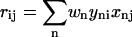
Following Kabsch's nomenclature (28), let us assume that we have two proteins X and Y, both having n atoms. The centers of mass of both proteins are at the origin (it is trivial to translate any set of protein coordinates to accomplish this). If we wish to rotate protein X to best match the coordinates of protein Y, we start by calculating a 3 × 3 covariance matrix (R) between the two set of points X and Y where i and j denote the three-dimensional components of each atom n and

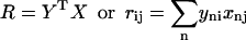(1)

The square of the covariance matrix (R²) is calculated as

(2)

The eigenvectors (A) and eigenvalues of R² are determined and sorted in decreasing order of eigenvalues. The normalized product of (R × A) is denoted as matrix B. Matrices A and B are used to calculate the rotation matrix (U) where

(3)

All coordinates of protein X are rotated to produce coordinates X′.

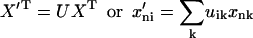(4)

These new coordinates X′ are compared back to coordinates Y of protein Y. The sRMSD is calculated as follows

(5)

where

(6)

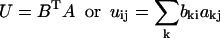
Weighted RMSD fit

We use a Gaussian-weighting factor in the wRMSD procedure. The weight is given by

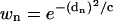(7)

where c is an arbitrary scaling factor and d_n is determined with Eq. 6. It should be noted that d is the distance between atom n in each protein conformation (X and Y). The distance is not between two atoms (n and m) in the same protein, nor is it a comparison of the n–m distance in conformations X and Y.

The weighted term is incorporated into the calculation of a weighted center of mass (Eq. 8), and this term is used to orient the weighted center of mass of each protein at the origin.

(8)

An sRMSD fit minimizes the sum of but a wRMSD fit minimizes the sum of Kabsch noted that weighting terms can be used in the RMSD fit by simply incorporating them into the covariance matrix.

(9)

At this point, the procedure is the same. The eigenvectors of R² are found and used with R to produce the rotation matrix U (Eqs. 2–4).

The sRMSD from Eq. 5 is rewritten as a weighted RMSD.

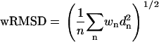(10)

A second metric can be created from a sum of all weights. The maximum value occurs when all weighs are 1.0 and the sum is n (all atom pairs are perfectly overlaid). The number of atoms will vary for each protein system, so a normalized measure is more appropriate. We write the sum of all weights (%wSUM) as

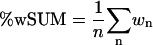(11)

Technically, it may be more appropriate to calculate wRMSD as the square root of the sum of divided by the sum of w_n. However, we found that Eq. 10 better reflects the agreement in the overlay. If the user desires to calculate wRMSD in the alternate fashion, it is simply wRMSD from Eq. 10 divided by the square root of %wSUM in Eq. 11.

We verified that our code produced proper sRMSD fits before incorporating the weighted terms. We also confirmed that when the scaling factor c is set to a very high number (10⁴ or higher), the weights become approximately one for all atom pairs, and a sRMSD fit is produced.

It should be noted that Diamond also outlined how weights could be included in his alignment process (53). Our Gaussian weighting idea could also be added to any code based on Diamond's approach by following the discussions in that work. Neither Kabsch nor Diamond ever define how weights should be calculated, and to the best of our knowledge, no one has published a weighted alignment using either Kabsch's or Diamond's methods. Even Diamond's proposal for overlaying ensembles of NMR structures (54) does not weight the contributions of different atom pairs. In that application, subsets of Cα are simply described as “in” or “out” of the overlay process. However, that application does show how alignments can be extended to ensembles of structures, through iteratively fitting N structures in N(N − 1)/2 pairs until convergence is achieved. For simplicity, our code in the Supplementary Material and our examples in this article use only two conformations of each protein, but this code could be inserted into any program that iteratively aligns ensembles of structures.

Another issue that deserves discussion is the importance of coordinate accuracy. Schneider (24,25) developed a method for aligning two protein conformations, which analyzes the interatomic distances within each independent protein structure to determine subsets of atoms to use in an sRMSD alignment. A unique caveat is his use of a weighting term, biased by coordinate accuracy, to define the subset for the alignment. (Though weights are used to define the subset, the weights are not part of the sRMSD.) Our implementation of wRMSD indirectly accounts for coordinate accuracy. The coordinate uncertainty is highest in the flexible regions of the protein, and the flexible regions of the protein are inherently underweighted in our implementation. According to Diamond (53), the errors would have to be on the order of the coordinate measurement itself to be significant. In our implementation, the errors would have to be on the order of Ångstroms (similar to the scaling factor c), which only happens in poorly resolved loop regions.

Alignment method

Our code currently implements our method using Cα coordinates of two protein conformations (it is straightforward to use all atoms, only backbone atoms, etc.). The procedure requires three steps: first, create a list of corresponding atom pairs; second, perform an initial sRMSD alignment to bring the two proteins into proximity; third, conduct iterative wRMSD fitting until convergence is reached. Our method can be used to align two conformations of the same protein, but aligning two homologs could be accomplished by incorporating some initial sequence or structural comparison to create the corresponding atom pairs.

The first step in our alignment method is to compare the residues of proteins X and Y. This is done to ensure that each residue is present in both structures and can be included in the alignment. A residue identification (ID) list is parsed for both proteins from its respective PDB file. A residue ID is included only if the residue has Cα atomic coordinates in both structures. Next, we remove any inappropriate residues from the residue ID lists, which include duplicate residues, disordered residues, or heterogroups. Duplicate and disordered residues are typically the result of alternative conformations revealed by the electron density maps. As our method inherently underweights flexible regions, it is justified to remove these residues from the alignment. The Cα coordinates that correspond to the residues remaining in the residue ID lists are parsed from their respective PDB files and used for the initial sRMSD alignment.

An sRMSD alignment (nonweighted) is performed first to bring the structures into close proximity to calculate an appropriate weighted alignment. Consequently, an atom's initial Gaussian weight is based on the distance between its positions in protein X and protein Y, calculated after the sRMSD fit. The Gaussian-weighted alignment is then performed in an iterative manner until convergence is reached (Fig. 1). Each iteration recalculates an appropriate weighted center of mass and a new rotation matrix.

FIGURE 1.

A series of iterations are needed to converge the wRMSD solution for overlaying two proteins. Four snapshots from the series of iterations are shown to demonstrate the process. The Supplementary Material provides a movie of all 24 iterations required for convergence of the GroEL system.

RESULTS AND DISCUSSION

Gaussian-weighted RMSD alignment

A weighted alignment is not as straightforward as a standard alignment. The structures must be nearly aligned to calculate appropriate weights, hence our use of an initial sRMSD alignment. Fig. 1 shows that the wRMSD procedure requires successive iterations until convergence is achieved because every wRMSD fit changes the distances, which changes the weights, which changes the wRMSD fit. To evaluate convergence, a metric is needed to describe optimal partial alignment. Proper metrics are even more important with wRMSD because a weighted alignment does not have a unique solution like an sRMSD fit. If we align the same protein on itself, there are two minima where the sum of is zero. The first occurs when the difference between all atom pairs is zero, and the protein is perfectly overlaid (all ); the second minimum happens at infinite separation when all weights go to zero (all w_n = 0).

It was previously shown that there is generally not a unique solution when calculating a global alignment of dynamic proteins (55). By determining a metric to identify an optimal partial alignment, we can fully automate our method and remove the subjectivity of evaluating the RMSD fit by visual inspection. We have chosen to explore two different metrics in detail: the wRMSD of Eq. 10 and the %wSUM given in Eq. 11. The wRMSD decreases to a stable minimum, while the %wSUM increases to a stable maximum. The optimal solution should occur when the maximum number of atoms makes a significant contribution. Hence, in our example of the wRMSD alignment of a protein upon itself, %wSUM identifies the perfectly overlaid minimum to be more significant because more atoms are contributing significantly to the weights (%wSUM = 1). The infinitely separated minimum has a %wSUM = 0.

Gaussian scaling factor

We started by investigating the most appropriate way to weight the RMSD fit. The Gaussian scaling factor c in Eq. 7 controls the weight given to a pair of Cα atoms. For instance, a Cα pair that is 1 Å apart will have a weight of 0.368 with c = 1 Ų. If c = 5 Ų, the weight is 0.819. Smaller values of c result in tighter, more restrictive coupling that forces only very similar atoms to have significant weights during the wRMSD fit.

We found that performing the weighted alignment in an iterative manner with a constant scaling factor exhibits converging behavior. We defined convergence by ΔwRMSD < 1 × 10⁻⁶ Å. This behavior is illustrated in Fig. 2 A using the ERα structures (37) 3ERD and 3ERT (scaling factor c set to 2 Ų). After 19 iterations, both the wRMSD and %wSUM metrics converge to stable values of 0.36 Å and 74.8%, respectively. In the final alignment, 182 of the 238 Cα common to both structures are within 1 Å, and the average distance between all 238 Cα pairs is 2.0 Å. The same converging behavior was also observed for all other test cases. Fig. 2, B and C, show a standard and Gaussian-weighted alignment of ERα. Arrows in Fig. 2 C highlight the improvement in aligning the rigid core of ERα.

FIGURE 2.

ERα (37). (A) The behavior of the wRMSD and %wSUM metrics as the weighted alignment is performed in an iterative manner using the entire protein sequence for the initial sRMSD fit. A scaling factor of 2 Ų is used. The vertical line indicates where convergence is reached. (B) sRMSD alignment of 3ERD (light gray) onto 3ERT (dark gray). (C) wRMSD alignment after convergence is reached. Arrows denote regions with improved fit.

We varied the scaling factor, using c-values from 0.10 to 20 Ų, to determine its effect on the weighted alignment. We found that upon convergence a range of c-values produced nearly identical alignments. This was determined by calculating the sRMSD of each solution. As shown in Fig. 3 using the ERα structures (37) 3ERD and 3ERT, the sRMSD remained relatively constant for c in the range of 0.3–20 Ų. The constant regions were defined as the change in sRMSD (ΔsRMSD) of <0.1 Å from the maximum to the minimum value in the range. The reader will notice that the sRMSD of 5.2 Å is higher than the 4.9 Å listed for the ERα structures in Table 1. This is appropriate; an sRMSD measurement from a wRMSD fit should be higher because some fit of flexible regions is sacrificed to better align the rigid core.

FIGURE 3.

The scaling factor, c, plotted against the sRMSD value for each weighted fit and the target coordinates. Open squares (□) are for ERα (37), 3ERD fit onto 3ERT. The weighted fit is the same for c-values from 0.3 to 20 Ų. Solid triangles (▴) are for PKA (33,34), 1JLU fit onto 1CMK. The weighted fit is the same for c-values from 0.2 to 2 Ų. The largest values of c simply reproduce the sRMSD solution for the PKA structures.

For the PKA structures 1JLU and 1CMK (33,34), the sRMSD stayed constant for a much smaller range of c-values, 0.2–2 Ų, as illustrated in Fig. 3. In the case of PKA, high values of c (≥10 Ų) simply produce the sRMSD solution (the later values of sRMSD in Fig. 3 are 1.9 Å, the same as the value in Table 1).

Table 3 shows the range of optimal c-values for each protein system (represented by its sRMSD) along with the ΔsRMSD value. We found a correlation between the sRMSD and the optimal scaling factor for wRMSD. When the structures are very similar (characterized by a small sRMSD), a smaller scaling factor is required to obtain a “tighter fit” of the rigid core. A scaling factor equal to 2 Ų performs well for all systems except RNA Pol, corresponding to the largest sRMSD. We suggest that when the sRMSD is <5 Å, a scaling factor of 2 Ų should be used, and sRMSD above 5 Å requires a scaling factor of 5 Ų.

TABLE 3.

Range of optimal scaling factors for each protein system, along with the calculated sRMSD of the wRMSD fit over the given range

Protein system	sRMSD from the wRMSD fit (Å)	Range of c (Å2) that produce the same sRMSD*
HIV-1p	1.4	2–5
PKA	2.3	0.2–2
EFG	3.6	0.2–4
ERα	5.2	0.3–20
DNA Pol†	7.2, 7.6	2–3, 4–6
GroEL	15.9	2–16
RAN	16.8	0.5–20
RNA Pol	20.6	3–20

^*The values for sRMSD changed <0.1 Å over the noted range.

^†The DNA Pol system converged to two different solutions when c was changed. Both were stably converged over the noted ranges.

If the scaling factor used is too small for the particular system, we do not see converging behavior, and an optimal solution is never reached. Fig. 4 demonstrates this issue using the GroEL system (39,40). In Fig. 4 A, when the c is equal to 1 Ų, we do not see converging behavior. The resulting alignment after 800 iterations is shown in Fig. 4 B. This unconverged alignment is very similar to the sRMSD alignment used to start the wRMSD fit. However, when a larger scaling factor is used (c = 5 Ų), we observe convergence after 93 iterations as shown in Fig. 4, A and C.

FIGURE 4.

If the scaling factor is too small, the wRMSD fit fails to produce converged structures for GroEL (39,40). (A) The behavior of the wRMSD metric versus iteration during the weighted fit, using the entire protein sequence for the initial RMSD fit and two values of c. (B) wRMSD alignment of 1AON (light gray) onto 1OEL (dark gray) after 800 unconverged iterations of wRMSD fitting, c = 1 Ų. (C) wRMSD alignment of 1AON (light gray) onto 1OEL (dark gray) after convergence is reached, c = 5 Ų.

Fig. 5 uses elongation factor G (EFG) (35,36) to show the problem that occurs when c is too large. Large scaling factors produce a superposition similar to the standard alignment. Fig. 5 A shows a sRMSD alignment, and Fig. 5 B corresponds to a wRMSD fit with a scaling factor of 100 Ų. The reader can see that the alignments are basically identical. Fig. 5 C shows that the wRMSD alignment using a scaling factor of 2 Ų is able to highlight the similarity of the rigid core region.

FIGURE 5.

If the scaling factor is too large, a wRMSD fit is the same as an sRMSD fit for EFG (35,36). (A) sRMSD alignment of 1FNM (light gray) onto 2EFG (dark gray). (B) wRMSD alignment of 1FNM (light gray) onto 2EFG (dark gray) after convergence is reached, c = 100 Ų. (C) wRMSD alignment of 1FNM (light gray) onto 2EFG (dark gray) after convergence is reached, c = 2 Ų.

In all cases, the weighted alignment resulted in an improved fit over the standard alignment. However, the improvement is minimal when the two conformations of a protein are very similar (i.e., HIV-1p). When the sRMSD is small, the conformational change is only slight. This means that most of the calculated weights are approximately equal to one unless an incredibly small value is used for c. A figure in the Supplementary Material shows the difference in sRMSD and wRMSD alignments for HIV-1p (31,32). The wRMSD still biases the rigid core (most noticeable for the C-terminus at the bottom of the structure), but the overall effect on the system is slight. Representative sRMSD and wRMSD alignments are also given for RAN (41,42) and RNA Pol (43,44). A scaling factor of 2 Ų was used for all systems with an sRMSD <5 Å, and c = 5 Ų was used for systems with an sRMSD >5 Å.

Identifying domains and hinge regions

Inspection of the wRMSD alignment of EFG (35,36) in Fig. 5 C clearly shows that two possible solutions should exist: one where the upper domain is aligned and one where the lower domain is aligned. This inspired us to modify the technique in an effort to identify domains and hinge regions. This is possible if we change the initial sRMSD alignment.

As previously mentioned, the Gaussian weights are a direct result of the difference between the transformed atom pairs, calculated from the initial sRMSD fit. If the sRMSD alignment is performed using a select subset of the protein, this changes the weights and biases the wRMSD fit. In a way, we are taking advantage of the fact that a wRMSD fit has more than one minimum. Diamond suggested using multiple starting orientations to search for alternate solutions to an overlay (54), and we chose to align different sections of the protein as starting points to provide multiple solutions that can be ranked by the metrics previously discussed. This method will allow us to align different regions of the protein and identify common domains and linker regions.

We chose to generate 10 initial sRMSD alignments based on local regions of the proteins. The initial standard alignment used 10 residues, chosen evenly spaced through the sequence. When larger sections are used (i.e., 20 residues), we found that the initial alignment could be based on two different mobile regions simultaneously. In such a case, the weighted alignment would not converge to a successful solution. We also found that evenly spacing our 10 local regions (i.e., 10 residues from every 10% section of the sequence) appears to adequately sample the entire protein structure (at least for the diverse test set used here). Making more than 10 initial alignments through choosing more frequent sections of the sequence yielded the same optimal alignments (data not shown).

After the initial local alignments, the 10 starting structures were refined with iterative wRMSD calculations in our regular way using the entire protein chain. The Gaussian scaling factor was set to a small value to maintain the local bias, c = 2 Ų. This resulted in 10 final, weighted alignments. The %wSUM was plotted against the iteration number for each test case. As previously mentioned, the %wSUM should increase to a stable maximum value corresponding to an optimal solution where the maximum number of atoms makes the most significant contribution. When starting from different subsets of the protein sequence, the alignment of the largest domain corresponded to the solution with the largest %wSUM value. Aligning the second largest domain lead to the second largest %wSUM value, and so on. This behavior was expected, and it was observed for all test cases. Below we demonstrate the technique on EFG, RAN, and DNA Pol.

Fig. 6 A shows a plot of the %wSUM versus iteration number using the protein system EFG (35,36). Clearly, using small subsets of the protein in the initial sRMSD leads to the identification of the two different domains. The weighted alignment based on the largest domain of EFG, shown in Fig. 6 B, converged to the maximum %wSUM value (55.5%). Seven of the 10 local alignments (residues taken from 1 to 358) converged to this same solution. In Fig. 6 C, an alignment based on the smaller domain of EFG is shown. This second solution has a smaller %wSUM (27.1%) as expected. Three of the 10 local alignments converged to this second solution. The later solutions were initially aligned by sRMSD of residues 407–416, 465–474, and 523–532.

FIGURE 6.

EFG (35,36). (A) The behavior of the %wSUM metric as the weighted alignment is performed in an iterative manner. Ten different subsets of 1FNM (light gray) were used for the initial standard alignment onto 2EFG (dark gray) and then the weighted iterations were performed using the entire sequence (c = 2 Ų). (B) wRMSD alignment corresponding to the maximum %wSUM value. (C) wRMSD alignment corresponding to the smaller %wSUM value.

In the case of RAN (41,42), the final weighted alignments from seven of the 10 local alignments (residues 1–10, 41–50, 81–90, 101–110, 121–130, 141–150, and 161–170) converged to the maximum %wSUM value (55.5%), shown in Fig. 7 A. The corresponding alignment is found in Fig. 7 B where the largest domain of the protein is superimposed between the conformations. Our technique is even capable of the difficult task of finding an alignment based on RAN's N-terminal helix, given in Fig. 7 C. This alignment corresponds to residues 181–190 in Fig. 7 A and has a much smaller %wSUM (4.9%) than the first seven weighted alignments, as expected. The local alignments using residues 21–30 and 61–70 were to less structured regions of the protein, and the weighted alignments essentially converged to solutions with %wSUM near zero. Poor convergence and near-zero values indicate loop or hinge regions of a protein.

FIGURE 7.

RAN (41,42). (A) The behavior of %wSUM as the weighted alignment is performed in an iterative manner. Ten different subsets of 1RRP (light gray) were used for the initial standard alignment onto 1BYU (dark gray) and then the weighted iterations were performed using the entire sequence (c = 2 Ų). (B) wRMSD alignment corresponding to the maximum %wSUM value. (C) wRMSD alignment corresponding to the second largest %wSUM value.

DNA Pol is a very large protein with almost 900 residues and multiple domains (38). Using subsets of the protein for the initial sRMSD, we were able to find four distinct alignments based on different regions of the protein. The weighted alignments from three of the 10 local alignments (residues 446–455, 624–633, 713–722) converged to the maximum %wSUM value (32.7%), shown in Fig. 8 A. The resulting alignment is given in Fig. 8 B and is based on the largest region of DNA Pol. The alignment from the second solution (%wSUM = 32.1%) is shown in Fig. 8 C and corresponds to the weighted alignment based on five of the 10 local alignments (residues 1–10, 90–99, 179–188, 268–277, and 357–366). The alignments from the first two solutions are not the same; however, they share a common domain that is superimposed in both overlays. Two of the 10 local alignments (residues 802–811) converged to a third solution (17.3%), based on a different region of DNA Pol than the first two solutions. The resulting alignment is given in Fig. 8 D. The fourth solution is found in Fig. 8 E, and it was initially aligned by sRMSD of residues 534–544. The weighted alignment is based on a small region of secondary structure, and it has the lowest %wSUM (7.9%).

FIGURE 8.

DNA Pol (38). (A) The behavior of %wSUM as the weighted alignment is performed in an iterative manner. Ten different subsets of 1IH7 (light gray) were used for the initial standard alignment onto 1IG9 (dark gray) and then the weighted iterations were performed using the entire sequence (c = 2 Ų). The four distinct solutions are indicated on the right. (B) wRMSD alignment corresponding to the maximum %wSUM value. (C) wRMSD alignment corresponding to the second largest %wSUM value. (D) wRMSD alignment corresponding to the third largest %wSUM value. (E) wRMSD alignment corresponding to the smallest %wSUM value. This overlay is oriented differently than in panels B–D. Arrows in panels B–E highlight regions with good alignment.

The optimal local alignments shown in Figs. 6 B and 7 B are basically identical to the global wRMSD alignments started from the sRMSD fit of the entire structure. Table 4 shows that this trend was seen for all of the protein systems as demonstrated by the comparison of the global wRMSD fit and the best wRMSD fit from local alignments, as defined by highest %wSUM. In the case of DNA Pol, two solutions had been found when examining the appropriate values for c to report in Table 3. The alignment corresponding to the largest %wSUM value (32.7%, Fig. 8 B) was found to be identical to the global fit with c = 2 Ų. However, the second largest %wSUM value (32.1%, Fig. 8 C) matched the global wRMSD fit with c = 5 Ų.

TABLE 4.

A comparison of the wRMSD fits using an initial global sRMSD alignment and the best result from initial local alignments

Protein system	Difference in sRMSD (Å) between global and local wRMSD fits	Global scaling factor
HIV-1p	0	c = 2 Å2
PKA	0	c = 2 Å2
EFG	0	c = 2 Å2
ERα	0	c = 2 Å2
DNA Pol	0 (Fig. 9 B), 5.90 (Fig. 9 C)	c = 2 Å2
DNA Pol	5.71 (Fig. 9 B), 0.23 (Fig. 9 C)	c = 5 Å2
GroEL	0	c = 5 Å2
RAN	0	c = 5 Å2
RNA Pol	0.25	c = 5 Å2

Two local wRMSD fits for DNA Pol are compared to two global wRMSD fits.

Using wRMSD to evaluate protein structure predictions

The act of evaluating a predicted protein structure against its experimentally determined target is another example of comparing two conformations of the same protein sequence. To show how wRMSD can be used to evaluate a predicted structure, we examined five systems used in the CASP5 competition (45). The targets were chosen based on increasing difficulty: Target 179 (comparative modeling), Target 172 (comparative modeling/fold recognition), Target 170 (fold recognition/new fold), Target 147 (fold recognition), and Target 162-3 (new fold). These specific targets were discussed in several articles that assessed the community's performance as a whole (56–58). Each of these assessment articles relied heavily on the GDT_TS (Global Distance Test_Total Score) metric in their ranking of submitted predictions. The GDT_TS values discussed here were obtained from the CASP5 website (http://predictioncenter.org/casp5/Casp5.html).

Like other techniques in the literature, the GDT procedure evaluates two structures based on an sRMSD fit of a subset of atoms (59), but what makes GDT unique is that it is implemented to provide a type of weighted evaluation in its final GDT_TS value. GDT is an iterative method that determines the maximum number of residues that can be sRMSD fit within a given distance (i.e., performs an sRMSD overlay of all atoms in the structure that can be simultaneously superimposed within 0.5 Å, 1 Å, 1.5 Å, 2 Å… up to 10 Å). GDT uses many starting alignments and an iterative procedure to identify the optimal sRMSD alignment of the largest subset possible. The GDT_TS score is based on the percent of atoms that can contribute to a particular sRMSD alignment: GDT_TS = (P₁ + P₂ + P₄ + P₈)/4 where P_m is the percent of atoms that sRMSD fit within m Å. In the GDT_TS value, the atoms within 1 Å agreement have a weight of 100% in the GDT_TS; atoms within 2 Å, 4 Å, and 8 Å have weights of 75%, 50%, and 25%, respectively. The GDT technique can be used to create RMS/coverage graphs (29) by plotting the percentage of atoms (P_m) versus the cutoff m. As the cutoff m increases, P_m also increases.

Comparing a predicted structure to its target involves more structural variation than the comparison of two related crystal structures. As one might expect, we found that larger scaling factors were necessary to provide accurate comparisons. Paralleling our study of flexible proteins, we again found that a smaller scaling factor (c = 5 Ų) was necessary for easy targets with small deviations and larger values (c = 12 Ų) were needed for hard targets with greater differences. The figures below provide a scale to show how the distances (d_n) compare with their corresponding weights for c = 5 or 12 Ų. This allows the reader to compare the wRMSD weights in the figures to those of GDT_TS noted above. The wRMSD technique can also be used to create RMS/coverage graphs by plotting the %wSUM versus c. As the scaling factor c increases, %wSUM also increases in a manner similar to RMS/coverage graphs from GDT (see Supplementary Material).

Overall, the GDT_TS metric is the most representative measure of a prediction, and it is the most widely accepted evaluation tool (45,56–58). However, its rankings do not always match manual/visual rankings of challenging targets like new folds and difficult fold recognition cases (57). In particular, Aloy et al. (58) found that GDT_TS overranked “fragment” submissions that provided coordinates for only a portion of the sequence. To prevent a similar bias in our use of wRMSD, we provide a %wSUM score based on the fit of the coordinates in the prediction (n in Eq. 11 equals the number of atoms in the prediction) and a %wSUM_ALL, which corrects for any omitted coordinates (n in Eq. 11 equals the number of atoms in the target). If a prediction provides all Cα coordinates, %wSUM and %wSUM_ALL are equal. If some are omitted, %wSUM_ALL will be proportionally less than %wSUM. (For a more accurate comparison, %wSUM_ALL is used in our RMS/coverage graphs in the Supplementary Material).

Target 179 is the “easiest” target included in our study. Many of the teams provided submissions that closely resembled the target. We randomly chose five exceptional submissions, two good/moderate submissions, and five poor submissions. Table 5 shows that the ranking provided by %wSUM_ALL matches that of GDT_TS with the exception of groups 32 and 400. Fig. 9, A and B, shows the wRMSD alignment of teams 427's and 32's top-ranked predictions. The regions in blue and green have high weights and are in excellent agreement with the target structure. The cause for 32's poor GDT_TS rank is unknown. The CASP5 website gives the low rank and also provides a weak RMS/coverage plot (see Supplementary Material), but the values for P₁, P₂, P₄, and P₆ listed from the GDT_TS analysis do not match the plot and indicate that the GDT_TS score should be >85. It appears that there may have been a simple typographical or data processing error. The other good predictions look very similar to the alignments in Fig. 9, A and B; the differences are minor and are localized in the two red, low-weight regions. Teams 529, 291, 400, and 183 provided significantly fragmented submissions, and the %wSUM_ALL does not match %wSUM in those cases. Without the correction of %wSUM_ALL, team 529 would have been ranked too high. Fig. 9, C and D, shows that 400 should be higher ranked than 183 because the lowest part of the β-sheet region has better agreement and higher weights.

TABLE 5.

Target 179 wRMSD rankings (c = 5 Ų) compared to GDT_TS values

Group	%wSUM_ALL	%wSUM	GDT_TS
427	76.6	76.6	86.95
32	76.5	77.0	28.65
246	76.3	76.3	86.68
471	75.8	75.8	85.77
270	74.6	74.6	84.40
16	64.0	64.0	77.47
529	63.8	75.1	72.08
291	24.0	37.4	34.12
400	18.9	32.6	29.11
183	16.3	19.1	29.29
531	5.6	5.6	11.13
139	4.4	4.4	7.21

FIGURE 9.

The wRMSD alignments of (A) group 427's and (B) group 32's predictions (thick, colored lines) to Target 179 (thin, gray line). The wRMSD alignments of (C) group 400's submission and (D) group 183's submission are given as examples of the comparison of a fragment. The target has the same orientation in all alignments. (E) The scale at the bottom shows how smaller deviations (blue) are more heavily weighted in the wRMSD. Deviations over 3.9 Å have weights under 5% (red).

Target 172 has a central domain that a few teams predicted well; of those teams, we examined the submissions of groups 517 and 373. We also randomly chose four moderate submissions and four poor submissions. An interesting feature of the wRMSD local alignments is that alternate, lower-ranked overlays are also provided. Fig. 10, A and B, shows that the submission from group 517 has two solutions, one for the agreement in the central domain and a second solution showing a properly predicted helix in the more difficult domain, respectively. Two independent wRMSD solutions show that the two regions were properly solved, but not oriented in the correct relative positions. This example is simply provided to demonstrate a feature of the method. The second solution has a very low %wSUM_ALL, and its consideration is not necessary to properly rank the predictions of Target 172. Table 6 shows that the rankings from wRMSD match those of GDT_TS with the exception of the moderate submissions of groups 537 and 417. Fig. 11, A and B, shows that the difference in the rankings is due to small improvements in the weighted core and possibly the cumulative contributions of small weights in the large red region. However, the difference in ranks is small, and both groups 537 and 417 can be maximally aligned to highlight the good agreement in the same core region.

FIGURE 10.

The submission from group 517 to target 172 has two solutions (A) and (B) by wRMSD fitting. The second solution (B) is scored much lower because it is only a match of a small helix. The target (gray, thin line) is in the same orientation in both alignments. The color code of the weights is the same as in Fig. 10 E.

TABLE 6.

For Target 172, wRMSD rankings (c = 5 Ų) compared to GDT_TS values

Group	%wSUM_ALL	%wSUM	GDT_TS
517	33.2	33.2	46.50
373	22.0	22.0	31.83
537	19.3	22.9	25.85
417	19.0	20.6	26.20
40	18.8	30.7	25.00
56	15.5	36.4	22.27
513	7.5	8.4	17.32
282	4.8	5.3	10.50
180	3.7	3.7	8.53
397	1.4	17.6	2.99

FIGURE 11.

wRMSD fits for groups (A) 537 and (B) 417 to Target 172. The %wSUM_ALL values for the best wRMSD fit are given in parentheses. The color code of the weights is the same as in Fig. 10 E. The target (gray, thin line) is in the same orientation in both alignments.

Target 170 is a “new fold” target. It is considered a relatively straightforward example of the most difficult category (57,58). Predictions for these more challenging targets tend to have larger deviations, and a scaling factor of 12 was necessary. We found that alternate solutions became more common and more significant as the difficulty of the target increased. The submissions from the top chosen groups provided secondary alignments showing that more than one region of the structure was solved properly, but the regions were not correctly oriented relative to one another. This feature of the local wRMSD fitting is an advantage over using GDT, which does not provide alternate, lower-ranked solutions. Fig. 12, A–C, compares the multiple wRMSD solutions for the first three groups. wRMSD and GDT_TS have similar rankings for the best alignments (Table 7), except that the good submissions of groups 294 and 51 are switched. The best alignments of all groups match the central helix down the center of the structure, but groups 517 and 294 also provide a second helix in the correct relative positions. Group 51 does provide additional helical structure, but the orientation is not quite as good, and the weights are correspondingly lower (with scaling factors >20 Ų, the weights become more significant and group 51's submission is ranked highest; see Supplementary Material). The second solutions for groups 517 and 294 show that the third helix is properly predicted but misoriented relative to the first two helices. The third solution for group 517 shows additional agreement in the sheet region. This third solution has a low %wSUM_ALL and is an example of the borderline for a significant solution.

FIGURE 12.

The multiple wRMSD solutions for the top three structures chosen for Target 170 (thin, gray line). (A) The wRMSD alignments of team 517's prediction (thick, colored line). (B) The wRMSD alignment of team 400's fragment submission. (C) The solutions for team 51. The target has the same orientation in all alignments. (D) The scale shows the weights for these wRMSD fits based on c = 12 Ų. Deviations over 6.0 Šhave weights under 5% (red).

TABLE 7.

For Target 170, wRMSD rankings (c = 12 Ų) compared to GDT_TS values

Group	%wSUM_ALL	%wSUM	GDT_TS
517	43.1	43.1	53.26
294	43.0	43.0	51.45
51	41.4	41.4	51.81
373	31.9	31.9	40.94
45	28.3	28.3	39.86
28	25.2	25.2	36.96
80	25.1	25.1	35.51
61	13.2	20.2	26.81
314	10.7	10.7	19.56

Target 147 is a challenging case because of its classification and its size. Table 8 shows that the wRMSD alignment ranks entries 2, 29, 10, and 437 in agreement with the GDT_TS metric. All of the alignments have good %wSUM_ALL scores because of good to moderate agreement throughout much of the structure. Fig. 13, A, B, and D, shows the similar fits of the submissions for groups 2, 10, and 437 to the target, and Fig. 13 C shows the fit of the submission from group 331. We were surprised to see the structure from group 331 ranked so much higher with the %wSUM_ALL metric as compared to the GDT_TS metric. The 331 entry is pulled up in rank by wRMSD because it has excellent placement of three adjacent secondary structures (significantly blue regions in Fig. 13 C). With c = 12 Ų, there is still the intended bias of the method to identify local regions with exceptional agreement over a larger collection of residues with modest agreement. When the scaling factor is >20 Ų, the bias shifts toward matching more of the global structure, and 437 is ranked significantly higher than 331 (see Supplementary Material). The disagreement in the rank of entry 246 is not significant because of its low rank by both wRMSD and GDT_TS.

TABLE 8.

For Target 147, wRMSD rankings (c = 12 Ų) compared to GDT_TS values

Group	%wSUM_ALL	%wSUM	GDT_TS
2	24.7	24.7	33.44
29	19.2	19.2	27.57
10	12.6	12.6	24.36
331	11.8	12.9	16.66
437	11.0	13.0	21.80
52	5.9	8.7	9.62
246	5.3	5.3	12.07
64	4.1	7.4	7.16
25	3.6	20.7	4.28

FIGURE 13.

wRMSD fits for groups (A) 2, (B) 10, (C) 331, and (D) 437 (thick, colored lines) to Target 147 (gray, thin line). The %wSUM_ALL values for the best wRMSD fit are given in parentheses. The color code of the weights is the same as in Fig. 13 D. The target is in the same orientation in all alignments.

The most difficult target we investigated was 162. The third domain was classified as a new fold, and we focused our analyses on these residues in the submitted predictions. Table 9 shows that the best submissions are ranked highest but are in mixed order between wRMSD and GDT_TS. The rank order when c > 50 Ų appeared to be a good metric of a more global score. The groups rank 373 > 132 > 437 > 29 > 2 with this high scaling factor (Supplementary Material). This is in agreement with Aloy et al. (58) who ranked group 373 highest based on visual inspection, followed by group 132; groups 2 and 29 scored significantly below 373 and 132. It is encouraging that wRMSD with a larger scaling factor matches the rankings provided by visual inspection. Furthermore, the GDT_TS rank order is 132 >373 > 29 > 437 > 2, indicating that our larger-c calculation is not a simple reproduction of GDT_TS. Fig. 14 provides the best wRMSD solution for each of the top five submissions evaluated in this study. The entries are ordered by the “global” group rank noted above, but the alignments and weights are from a wRMSD fit with c = 12 Ų. This allows the reader to compare the structures for global and local characteristics. The best solutions have several pieces of secondary structure in proper relative locations. wRMSD fits have a short coming that is also seen in GDT_TS: matching a single long helix provides a relatively good score. The regular structure of a helix is simply easy to superimpose with good agreement (easier than superimposing a loop, turn, or twisted β-sheet that has more structural variation). The high score for helices simply reflects that they are the easiest substructure to properly predict.

TABLE 9.

For Target 162-3, wRMSD rankings (c = 12 Ų) compared to GDT_TS

Group	%wSUM_ALL	%wSUM	GDT_TS
29_3	19.9	34.4	23.512
2	17.8	17.8	20.238
437	17.3	19.1	22.173
132	16.7	16.7	24.405
373	16.2	16.2	24.107
397	13.8	34.5	18.452
282	10.8	12.6	15.923
227	10.4	25.1	14.435
180	7.3	7.8	12.649
291	6.8	9.1	10.268
196	6.0	20.1	7.589

FIGURE 14.

wRMSD fits for groups (A) 373, (B) 132, (C) 437, (D) 29, and (E) 2 to Target 162-3. The order A–E reflects a rank order based on the RMS/coverage graph, but the overlays and their weights are from a local wRMSD fit with c = 12 Ų. Two significant solutions were obtained for each group's entry but only the best is shown. The %wSUM_ALL values for the individual wRMSD solutions are given in parentheses. The color code of the weights is the same as in Fig. 13 D. The target (gray, thin line) is in the same orientation in all alignments.

CONCLUSION

Our Gaussian-weighted alignment tool has been successfully applied to many dynamic proteins with two known conformations. We have also shown that an sRMSD alignment for these proteins is usually inappropriate. Our method is capable of selecting out the static core regions of flexible proteins and returning an alignment heavily weighted by those coordinates.

We have developed two techniques to utilize our Gaussian-weighted method. The first, a global wRMSD fit, uses the entire protein sequence for an initial sRMSD alignment and performs iterative wRMSD fits of the entire structure with c = 2 or 5 Ų. When protein conformations are similar (sRMSD < 5 Å), c = 2 Ų is suggested. For larger conformational changes (sRMSD > 5 Å), the larger scaling factor is recommended. These values work well, allowing the wRMSD fit to converge to an appropriate solution.

Our second technique, a local wRMSD fit, uses subsets of the protein sequence for an initial, local sRMSD alignment and then performs a wRMSD fit of the entire protein, keeping the Gaussian scaling factor set to 2 Ų to maintain the local bias in the fit. The optimal solution is identified by the largest %wSUM. Using this second method, we were able to achieve multiple alignments based on different domains of the protein, and the solutions could be ranked by %wSUM.

Although a variety of alignment methods have previously been described to account for protein flexibility, we have developed a new method that is both general and robust. This method does not require any prior knowledge of the protein structure and removes the subjective nature of overlaying user-defined core regions of flexible proteins. This novel method can easily be incorporated into many RMSD overlay calculations.

Furthermore, we have shown how the local wRMSD technique can be used to evaluate protein structure predictions through an overlay with the experimentally determined target. The agreement with the standard GDT_TS metric is very good for most targets, with more variability in the rankings as the target becomes more difficult. The overlays provided by wRMSD are compeling for comparative modeling and fold recognition targets. Comparing predictions to new fold targets and more difficult fold recognition targets can provide more than one solution, highlighting cases where local, secondary, and tertiary structure is properly assigned but misoriented relative to one another. The %wSUM_ALL metric appears to be a good measure of global accuracy of a difficult target when the scaling factor is larger (∼50 Ų), and it is not a simple reproduction of the GDT_TS metric. By varying the scaling factor and examining the multiple solutions, the user can evaluate predictions for both local and global accuracy.

SUPPLEMENTARY MATERIAL

An online supplement to this article can be found by visiting BJ Online at http://www.biophysj.org. The Supplementary Material provides sRMSD and wRMSD alignments of two conformations of HIV-1p, RAN, and RNA Pol; the RMS/coverage graphs for each of the protein-prediction targets; the global and local wRMSD codes; and a movie of all the iterations generated in the wRMSD alignment of the two conformations of GroEL (only four of 24 iterations are shown in Fig. 1).

References

- 1.Tsai, C. J., S. Kumar, B. Ma, and R. Nussinov. 1999. Folding funnels, binding funnels, and protein function. Protein Sci. 8:1181–1190. [DOI] [PMC free article] [PubMed] [Google Scholar]
- 2.Ma, B., M. Shatsky, H. J. Wolfson, and R. Nussinov. 2002. Multiple diverse ligands binding at a single protein site: a matter of pre-existing populations. Protein Sci. 11:184–197. [DOI] [PMC free article] [PubMed] [Google Scholar]
- 3.Jeffery, C. J. 2004. Molecular mechanisms for multitasking: recent crystal structures of moonlighting proteins. Curr. Opin. Struct. Biol. 14:663–668. [DOI] [PubMed] [Google Scholar]
- 4.Finocchiaro, G., T. Wang, R. Hoffmann, A. Gonzalez, and R. C. Wade. 2003. DSMM: a database of simulated molecular motions. Nucleic Acids Res. 31:456–457. [DOI] [PMC free article] [PubMed] [Google Scholar]
- 5.Chiang, R. A., E. C. Meng, C. C. Huang, T. E. Ferrin, and P. C. Babbitt. 2003. The structure superposition database. Nucleic Acids Res. 31:505–510. [DOI] [PMC free article] [PubMed] [Google Scholar]
- 6.Gerstein, M., and W. Krebs. 1998. A database of macromolecular movements. Nucleic Acids Res. 26:4280–4290. [DOI] [PMC free article] [PubMed] [Google Scholar]
- 7.Krebs, W. G., and M. Gerstein. 2000. The morph server: a standardized system for analyzing and visualizing macromolecular motions in a database framework. Nucleic Acids Res. 28:1665–1675. [DOI] [PMC free article] [PubMed] [Google Scholar]
- 8.Echols, N., D. Milburn, and M. Gerstein. 2003. MolMovDB: analysis and visualization of conformational change and structural flexibility. Nucleic Acids Res. 31:478–482. [DOI] [PMC free article] [PubMed] [Google Scholar]
- 9.Gerstein, M., and N. Echols. 2004. Exploring the range of protein flexibility, from a structural proteomics perspective. Curr. Opin. Chem. Biol. 8:14–19. [DOI] [PubMed] [Google Scholar]
- 10.Buck, E., and R. Iyengar. 2003. Organization and functions of interacting domains for signaling by protein-protein interactions. Sci. STKE. 209:Re14. [DOI] [PubMed] [Google Scholar]
- 11.Pawson, T., and P. Nash. 2003. Assembly of cell regulatory systems through protein interaction domains. Science. 300:445–452. [DOI] [PubMed] [Google Scholar]
- 12.Hilser, V. J., D. Dowdy, T. G. Oas, and E. Freire. 1998. The structural distribution of cooperative interactions in proteins: analysis of the native state ensemble. Proc. Natl. Acad. Sci. USA. 95:9903–9908. [DOI] [PMC free article] [PubMed] [Google Scholar]
- 13.Luque, I., and E. Freire. 2000. Structural stability of binding sites: consequences for binding affinity and allosteric effects. Proteins. S4:63–71. [DOI] [PubMed] [Google Scholar]
- 14.Carlson, H. A., and J. A. McCammon. 2000. Accommodating protein flexibility in computational drug design. Mol. Pharmacol. 57:213–218. [PubMed] [Google Scholar]
- 15.Freer, S. T., J. Kraut, J. D. Robertus, H. T. Wright, and N. H. Xuong. 1970. Chymotrypsinogen: 2.5 Å crystal structure, comparison with α-chymotrypsin, and implications for zymogen activation. Biochemistry. 9:1997–2009. [DOI] [PubMed] [Google Scholar]
- 16.Gerstein, M., and R. B. Altman. 1995. Average core structures and variability measures for protein families: application to the immunoglobulins. J. Mol. Biol. 251:161–175. [DOI] [PubMed] [Google Scholar]
- 17.Irving, J. A., J. C. Whisstock, and A. M. Lesk. 2001. Protein structural alignments and functional genomics. Proteins. 42:378–382. [DOI] [PubMed] [Google Scholar]
- 18.Wriggers, W., and K. Schulten. 1997. Protein domain movements: detection of rigid domains and visualization of hinges in comparisons of atomic coordinates. Proteins. 29:1–14. [PubMed] [Google Scholar]
- 19.Shatsky, M., R. Nussinov, and H. J. Wolfson. 2002. Flexible protein alignment and hinge detection. Proteins. 48:242–256. [DOI] [PubMed] [Google Scholar]
- 20.Kotlovyi, V., W. L. Nichols, and L. F. Ten Eych. 2003. Protein structural alignment for detection of maximally conserved regions. Biophys. Chem. 105:595–608. [DOI] [PubMed] [Google Scholar]
- 21.Jewett, A. I., C. C. Huang, and T. E. Ferrin. 2003. MINRMS: an efficient algorithm for determining protein structure similarity using root-mean-squared-distance. Bioinformatics. 19:625–634. [DOI] [PubMed] [Google Scholar]
- 22.Alexandrov, V., and M. Gerstein. 2004. Using 3D hidden Markov models that explicitly represent spatial coordinates to model and compare protein structures. BMC Bioinformatcs. 5:2. [DOI] [PMC free article] [PubMed] [Google Scholar]
- 23.Ye, Y., and A. Godzik. 2004. Database searching by flexible protein structure alignment. Protein Sci. 13:1841–1850. [DOI] [PMC free article] [PubMed] [Google Scholar]
- 24.Schneider, T. R. 2002. A genetic algorithm for the identification of conformationally invariant regions in protein molecules. Acta Crystallogr. D58:195–208. [DOI] [PubMed] [Google Scholar]
- 25.Schneider, T. R. 2004. Domain identification by iterative analysis of error-scaled difference distance matrices. Acta Crystallogr. D60:2269–2275. [DOI] [PubMed] [Google Scholar]
- 26.Nichols, W. L., G. D. Rose, L. F. Ten Eyck, and B. H. Zimm. 1995. Rigid domains in proteins: an algorithmic approach to their identification. Proteins. 23:38–48. [DOI] [PubMed] [Google Scholar]
- 27.Nichols, W. L., B. H. Zimm, and L. F. Ten Eyck. 1997. Conformation-invariant structures of the α1β1 human hemoglobin dimer. J. Mol. Biol. 270:598–615. [DOI] [PubMed] [Google Scholar]
- 28.Kabsch, W. 1976. A solution for the best rotation to relate two sets of vectors. Acta Crystallogr. A32:922–923. [Google Scholar]
- 29.Hubbard, T. J. P. 1999. RMS/coverage graphs: a qualitative method for comparing three-dimensional protein structure predictions. Proteins. S3:15–21. [DOI] [PubMed] [Google Scholar]
- 30.Berman, H. M., J. Westbrook, Z. Feng, G. Gilliland, T. N. Bhat, H. Weissig, I. N. Shindyalov, and P. E. Bourne. 2000. The protein data bank. Nucleic Acids Res. 28:235–242. [DOI] [PMC free article] [PubMed] [Google Scholar]
- 31.Reiling, K. K., N. F. Endres, D. S. Dauber, C. S. Craik, and R. M. Stroud. 2002. Anisotropic dynamics of the Je-2147-HIV protease complex: drug resistance and thermodynamic binding mode examined in a 1.09 Å structure. Biochemistry. 41:4582–4594. [DOI] [PubMed] [Google Scholar]
- 32.Spinelli, S., Q. Z. Liu, P. M. Alzari, P. H. Hirel, and R. J. Poljak. 1991. The three-dimensional structure of the aspartyl protease from the HIV-1 isolate BRU. Biochimie. 73:1391–1396. [DOI] [PubMed] [Google Scholar]
- 33.Madhusudan, E. A. Trafny, N. H. Xuong, J. A. Adams, L. F. Ten Eyck, S. S. Taylor, and J. M. Sowadski. 1994. cAMP-dependent protein kinase: crystallographic insights into substrate recognition and phosphotransfer. Protein Sci. 3:176–187. [DOI] [PMC free article] [PubMed] [Google Scholar]
- 34.Zheng, J., D. R. Knighton, N. H. Xuong, S. S. Tayor, J. M. Sowadski, and L. F. Ten Eyck. 1993. Crystal structures of the myristylated catalytic subunit of cAMP-dependent protein kinase reveal open and closed conformations. Protein Sci. 2:1559–1573. [DOI] [PMC free article] [PubMed] [Google Scholar]
- 35.Laurberg, M., O. Kristensen, K. Martemyanov, A. T. Gudkov, I. Nagaev, D. Hughes, and A. Liljas. 2000. Structure of a mutant EF-G reveals domain III and possibly the fusidic acid binding site. J. Mol. Biol. 303:593–603. [DOI] [PubMed] [Google Scholar]
- 36.Czworkowski, J., J. Wang, T. A. Steitz, and P. B. Moore. 1994. The crystal structure of elongation factor G complexed with GDP, at 2.7 Å resolution. EMBO J. 13:3661–3668. [DOI] [PMC free article] [PubMed] [Google Scholar]
- 37.Shiau, A. K., D. Barstad, P. M. Loria, L. Cheng, P. J. Kushner, D. A. Agard, and G. L. Green. 1998. The structural basis of estrogen receptor/coactivator recognition and the antagonism of this interaction by tamoxifen. Cell. 95:927–937. [DOI] [PubMed] [Google Scholar]
- 38.Franklin, M. C., J. Wang, and T. A. Steitz. 2001. Structure of the replicating complex of a Pol α family DNA polymerase. Cell. 105:657–667. [DOI] [PubMed] [Google Scholar]
- 39.Xu, Z., A. L. Horwich, and P. B. Sigler. 1997. The crystal structure of the asymmetric GroEL-GroES-(ADP)7 chaperonin complex. Nature. 388:741–750. [DOI] [PubMed] [Google Scholar]
- 40.Braig, K., P. D. Adams, and A. T. Brunger. 1995. Conformational variability in the refined structure of the chaperonin GroEL at 2.8 Å resolution. Nat. Struct. Biol. 2:1083–1094. [DOI] [PubMed] [Google Scholar]
- 41.Vetter, I. R., C. Nowak, T. Nishimoto, J. Kuhlmann, and A. Wittinghofer. 1999. Structure of a Ran-binding domain complexed with Ran bound to a GTP analogue: implications for nuclear transport. Nature. 398:39–46. [DOI] [PubMed] [Google Scholar]
- 42.Stewart, M., H. M. Kent, and A. J. McCoy. 1998. The structure of the Q69L mutant of GDP-Ran shows a major conformational change in the switch II loop that accounts for its failure to bind nuclear transport factor 2 (NTF2). J. Mol. Biol. 284:1517–1527. [DOI] [PubMed] [Google Scholar]
- 43.Cheetham, G. M. T., and T. A. Steitz. 1999. Structure of a transcribing T7 RNA polymerase initiation complex. Science. 286:2305–2309. [DOI] [PubMed] [Google Scholar]
- 44.Yin, Y. W., and T. A. Steitz. 2002. Structural basis for the transition from initiation to elongation transcription in T7 RNA polymerase. Science. 298:1387–1395. [DOI] [PubMed] [Google Scholar]
- 45.Moult, J., K. Fidelis, A. Zemla, and T. Hubbard. 2003. Critical assessment of methods of protein structure prediction (CASP)-Round V. Proteins. 53:334–339. [DOI] [PubMed] [Google Scholar]
- 46.Teplyakov, A., G. Obmolova, P. P. Khil, A. J. Howard, R. D. Camerini-Otero, and G. L. Gilliland. 2003. Crystal structure of the Escherichia coli YcdX protein reveals a trinuclear zinc active site. Proteins. 51:315–318. [DOI] [PubMed] [Google Scholar]
- 47.Yamashita, A., K. Maeda, and Y. Maeda. 2003. Crystal structure of CapZ: structural basis for actin filament barbed end capping. EMBO J. 22:1529–1538. [DOI] [PMC free article] [PubMed] [Google Scholar]
- 48.Allen, M., A. Friedler, O. Schon, and M. Bycroft. 2002. The structure of an FF domain from human HYPA/FBP11. J. Mol. Biol. 323:411–416. [DOI] [PubMed] [Google Scholar]
- 49.Miller, D. J., N. Ouellette, E. Evdokimova, A. Savchenko, A. Edwards, and W. F. Anderson. 2003. Crystal complexes of a predicted S-adenosylmethionine-dependent methyltransferase reveal a typical AdoMet binding domain and a substrate recognition domain. Protein Sci. 12:1432–1442. [DOI] [PMC free article] [PubMed] [Google Scholar]
- 50.Tan, A. Y., P. C. Smith, J. Shen, R. Xiao, T. Acton, B. Rost, G. Montelione, and J. F. Hunt. Crystal structure of spermidine synthase. http://pdbbeta.rcsb.org/pdb/explore.do?structureId=/IY9.
- 51.DeLano, W. L. The PyMOL Molecular Graphics System. 2002. DeLano Scientific, San Carlos, CA. http://www.pymol.org.
- 52.Flower, D. R. 1999. Rotational superposition: a review of methods. J. Mol. Graph. Model. 17:238–244. [PubMed] [Google Scholar]
- 53.Diamond, R. 1988. A note on the rotational superposition problem. Acta Crystallogr. A44:211–216. [Google Scholar]
- 54.Diamond, R. 1992. On the multiple simultaneous superposition of molecular structures by rigid body transformations. Protein Sci. 1:1279–1287. [DOI] [PMC free article] [PubMed] [Google Scholar]
- 55.Godzik, A. 1996. The structural alignment between two proteins: is there a unique answer? Protein Sci. 5:1325–1338. [DOI] [PMC free article] [PubMed] [Google Scholar]
- 56.Tramontano, A., and V. Morea. 2003. Assessment of homology-based predictions in CASP5. Proteins. 53:352–368. [DOI] [PubMed] [Google Scholar]
- 57.Kinch, L. N., J. O. Wrabl, S. S. Krishna, I. Majumdar, R. I. Sadreyev, Y. Qi, J. Pei, H. Cheng, and N. V. Grishin. 2003. CASP5 assessment of fold recognition target predictions. Proteins. 53:395–409. [DOI] [PubMed] [Google Scholar]
- 58.Aloy, P., A. Stark, C. Hadley, and R. B. Russell. 2003. Predictions without templates: new folds, secondary structure, and contacts in CASP5. Proteins. 53:436–456. [DOI] [PubMed] [Google Scholar]
- 59.Zemla, A. 2003. LGA: A method for finding 3D similarities in protein structures. Nucleic Acids Res. 31:3370–3374. [DOI] [PMC free article] [PubMed] [Google Scholar]