Mapping Tumor-Suppressor Genes with Multipoint Statistics from Copy-Number–Variation Data

Abstract

Array-based comparative genomic hybridization (arrayCGH) is a microarray-based comparative genomic hybridization technique that has been used to compare tumor genomes with normal genomes, thus providing rapid genomic assays of tumor genomes in terms of copy-number variations of those chromosomal segments that have been gained or lost. When properly interpreted, these assays are likely to shed important light on genes and mechanisms involved in the initiation and progression of cancer. Specifically, chromosomal segments, deleted in one or both copies of the diploid genomes of a group of patients with cancer, point to locations of tumor-suppressor genes (TSGs) implicated in the cancer. In this study, we focused on automatic methods for reliable detection of such genes and their locations, and we devised an efficient statistical algorithm to map TSGs, using a novel multipoint statistical score function. The proposed algorithm estimates the location of TSGs by analyzing segmental deletions (hemi- or homozygous) in the genomes of patients with cancer and the spatial relation of the deleted segments to any specific genomic interval. The algorithm assigns, to an interval of consecutive probes, a multipoint score that parsimoniously captures the underlying biology. It also computes a P value for every putative TSG by using concepts from the theory of scan statistics. Furthermore, it can identify smaller sets of predictive probes that can be used as biomarkers for diagnosis and therapeutics. We validated our method using different simulated artificial data sets and one real data set, and we report encouraging results. We discuss how, with suitable modifications to the underlying statistical model, this algorithm can be applied generally to a wider class of problems (e.g., detection of oncogenes).

The process of carcinogenesis imparts many genetic changes to a cancer genome at many different scales: point mutations, translocations, segmental duplications, and deletions. Whereas most of these changes have no direct impact on the cellular functions—and may not contribute to the carcinogenesis in any obvious manner—few of these chromosomal aberrations have a disproportionately significant impact on the cell’s ability to initiate and maintain processes involved in tumor growth; namely, through its ability to proliferate, escape senescence, achieve immortality, and signal to neighboring cells. Two classes of genes are critically involved in cancer development and are discernible in terms of their copy-number variations (CNVs): oncogenes that are activated or altered in function and tumor-suppressor genes (TSGs) that are deactivated in cancer cells. Thus, the effect of oncogenes is via gain-of-function mutations that lead to malignancy. For instance, a segmental amplification can increase the genomic copy number of a region containing an oncogene, thus leading to overexpression of the oncogene product. The mutation is dominant; that is, only a mutated allele is necessary for the cell to become malignant. TSGs affect the cells via mutations (often involving segmental deletions) that contribute to malignancy by loss of function of both alleles of the gene. The “two-hit” hypothesis of Knudson¹ for tumorigenesis has been widely recognized as an important model of such losses of function involved in many cancers.

Whole-genome–scale data and their computational analysis can now lead to rapid discovery and characterization of important genetic changes at significantly higher resolution, thus providing a systems-level understanding of the roles of oncogenes and TSGs in cancer development and its molecular basis. As an example, whereas BRCA1 and BRCA2 TSGs provide better understanding of familial breast cancer and other TSGs, including PTEN and p53, do so for sporadic breast cancer, we still lack a reasonably complete picture, since many important components remain undiscovered. Whole-genome analysis, now possible through array-based comparative genomic hybridization (arrayCGH) experiments, can remedy the situation by shedding light on many more genes and their interrelationship.

In the current whole-genome analysis setup, microarray techniques are being used successfully to measure fluctuations in copy number for a large number of genomic regions in one genome relative to a different but related genome sample. For example, arrayCGH can map copy-number changes at a large number of chromosomal locations in one genome with respect to a reference genome and, from them, extrapolate to infer segments of the genome that have undergone the same degree of amplifications or deletions. For some references to and discussions of algorithms that estimate these CNVs, see Daruwala et al.²

In the present article, we examine how these CNV data can be used for the purpose of identifying TSGs. The intuitive basis of our approach can be easily stated, as follows. Suppose we have whole-genome CNV data for several patients who suffer from the same specific class of cancer, putatively caused by loss of function in both alleles of the same TSG. In that case, the loss-of-function event may have many underlying causes; for instance, a nonsynonymous point mutation in the exon, a mutation in the regulatory region, a small insertion-deletion event in the coding region, or a relatively large segmental deletion event that affects one or many exons of the gene. In each case, the phenotypic result will be similar, but the whole-genome analysis will identify only segmental deletion events that exhibit themselves through reduced copy-number values for genomic intervals. For any such deleted segment to effect a loss of function in the TSG, it must overlap with the genomic interval corresponding to the TSG. Even though events representing small, undetectable mutations will go unnoticed, by accounting for the CNVs, a suitable algorithm can infer the location of the TSG implicated in the disease. Our approach exploits these topological relationships among the genomic intervals and works by enumerating all possible intervals in the genome and then evaluating them with a score function that measures the likelihood of an interval being exactly the TSG. The mathematical derivation and properties of this score function appear in the appendix (online only).

The rest of the article is organized as follows. We first present a formal description of the score function, which we have only intuitively sketched so far (see the “Methods” section), and then show how this function is used in evaluation of whether a region represents a TSG. Next, we illustrate our method, using this score function and several sets of simulated data, computed under a wide variety of scenarios (see the “Results” section); we also assess the power of the method by examining how accurately it discovers the true location (which is known to the simulator) of the TSG. Finally, we analyze and report the results from an arrayCGH data set (using 100K Affy-chips), obtained from several patients with lung cancer. We conclude with a discussion of the strength and weakness of the proposed method (see the “Discussion” section).

Methods

Our method for the identification of TSGs relies on a multipoint score function, computed over whole-genome–analysis data for a sufficiently large group of patients suffering from the same form of cancer. In the following section, we present a systematic derivation of this score function, starting with a few simple assumptions about the underlying biology and the data.

Definition of Relative Risk

For any interval I (represented as a set of consecutive probes), we wish to quantify the strength of the association between deletions in I and the disease by analyzing the genomic data for many diseased individuals. For this purpose, we select a metric, the relative risk (RR), as it compares and assigns a numerical value to the risks of disease in two populations with respect to each other: the first population comprises subjects whose genomes contain a segmental deletion in the interval I, and the second comprises subjects whose genomes have no such segmental deletion in I.

We caution the reader that, in an abuse of definition, we will frequently use the shortened phrase “I deleted” to mean that “at least a part of I is deleted.”

The first term in equation (1) can be estimated from the tumor samples available:

where n_{I deleted} (or n_{I NOTdeleted}) is simply the number of tumor samples in which I is deleted (or not deleted).

The second part of equation (1),

incorporates prior information inherent in the statistical distribution of deletions. For instance, we may note that if I is a small interval, then P(I deleted)≪P(I NOTdeleted) and, hence,

is a large positive number. Similarly, if I is very large, then the situation is reversed and

becomes a large negative number. Consequently, the prior information, included in the distribution of random unrelated deletions in the genome, is reflected through an advantage accrued to small intervals; in other words, under the assumption that the same strength of evidence exists in the data for different sizes, preference is given to the smaller intervals.

To derive a computational procedure for this prior score, we rely on a probabilistic model of how the genomic data may have been generated. In this simplest parsimonious model, we assume that, at any genomic location, a breakpoint may occur as a Poisson process at a rate of μ⩾0. At the places where any of these breakpoints start, a segmental deletion may occur, the length of which is distributed as an exponential random variable with a parameter λ⩾0. Note the following lemma.

Lemma 1.—Under the assumption of the generative process described above, the probability that an interval I=[a,b] (in the genome) is deleted can be expressed as

where [0,G] represents the region of interest (e.g., a chromosome) and [a,b] is a specific genomic interval in this region. See the appendix (online only) for proof of the lemma.

Using equations (2) and (3), we can now compute the score function RR_{I deleted} for an interval I. Parameters μ and λ, which appear in the score function, are assumed to have been estimated from data by a procedure described in the next section.

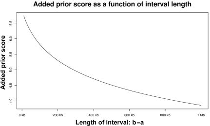
In figure 1, we show how the additional prior score

computed using equation (3) in the previous lemma, varies as a function of the length of the interval. All the parameters (μ, λ, and G) are the same as those in the simulation examples in the “Results” section. Figure 1 emphasizes the significantly higher prior advantage given to intervals of smaller length.

Figure 1. .

Prior score as a function of the length of the interval. A priori, shorter intervals receive higher weight than larger intervals.

Clearly, we expect the high-scoring intervals determined by this method to be treated as candidates for TSGs. We still need to define precisely how and how many of these intervals should be selected and then evaluated for their statistical significance.

Estimating Parameters

In the preceding section, we defined a score for an interval I (RR_{I deleted}), which depends on two extraneous parameters that describe a background genome-reorganization process. These two parameters—namely, λ and μ—must be estimated from arrayCGH data. We recall that λ is the parameter of the exponential distribution for generating deletions—that is,  1/λ is the average length of a deletion—and that μ is the parameter of the Poisson process used for generating the breakpoints—that is, μ is the mean number of breakpoints per unit length.

Recently, several statistically powerful algorithms have been devised to analyze the arrayCGH data and to render the underlying genome in terms of segments of regions of similar copy numbers. These algorithms readily yield an output that can be interpreted as alternating segments of normal and abnormal segments, with the abnormal segments falling into two groups: segmental losses and segmental gains. If these segments satisfy the assumptions regarding the breakpoint and length distributions, the desired parameters μ and λ can be estimated empirically from the segmentation of the data. Certain Bayesian algorithms, such as the one proposed by Daruwala et al.² and its variants (T. S. Anantharaman, M. Sobel, and B.M., unpublished data), include these assumptions in their prior and are thus able to estimate these parameters directly. The present algorithm builds on the latter class of segmentation algorithms but is not limited by this requirement.

In addition to estimating λ and μ, we also use the segmentation of individual samples to obtain the positions of the breakpoints (points where deletions start) in each sample and use these positions to assess the statistical significance of our results.

Estimating the Location of the TSG

The estimation procedure proceeds in a sequence of steps. In the first step, the algorithm computes the scores (RR_{I deleted}) for all the intervals I, with lengths taking values in a range determined by a lower and an upper bound, starting with small intervals containing a few markers and ending with very long intervals. We have evaluated two different statistical methods designed to estimate the location of the TSGs.

The first and the simplest method operates by simply choosing the maximum-scoring interval as the candidate TSG; namely, it selects the interval I with maximum RR_{I deleted} in a genomic region of interest (e.g., a chromosome or a chromosomal arm) as the most plausible location of a causative TSG. We refer to this method as the “Max method.”

The other method functions by estimating the locations of the left and the right boundaries of the TSG, with use of two scoring functions, as described below. Two scores, SL_x and SR_x, are computed for every marker position x∈[0,G]. The first value, SL_x, is to be interpreted as the confidence that the point x is the left boundary of a TSG; symmetrically, the latter, SR_x, is the confidence that the point x is the right boundary of a TSG. These scores are defined more formally as

where ℐℒ_x is the set of intervals that are bounded by the marker x from the left. Similarly,

where ℐℛ_x is the set of intervals with the right boundary exactly at x.

Using these two scores, we can obtain an estimation of the true position of the TSG as the interval [x^*_L,x^*_R], where, for the left (right) boundary, we choose the marker position () that maximizes the SL_x (SR_x) score. We refer to this method as the “LR method.”

Significance Testing

Thus far, we have seen how to estimate the putative location of a TSG either by maximizing the RR scores over many intervals or by estimating other related scores that characterize the boundaries of the gene. Irrespective of which method is chosen, the result is always an interval that consists of some number of markers; in the following, the computed interval is referred to as “I_max.” The final step of our algorithm determines whether this finding is statistically significant; that is, it assigns a P value to I_max.

Unfortunately, there is no obvious or readily available approach for analytically computing a P value for an interval I_max. Therefore, the algorithm must rely on a different empirical method to compute the statistical significance; namely, it computes the P value from the observed distribution of breakpoints along the chromosome (as given by the segmentation algorithm). It uses a null hypothesis that no TSG resides on the chromosome; consequently, the breakpoints can be expected to be uniformly distributed. Note that, if a detailed and complete understanding of a genomewide distribution of breakpoints were available, then it would pose little difficulty in changing the following discussions and derivations mutatis mutandis. However, to avoid any unnecessary biases in our estimators, we chose, for the time being, to focus on an uninformative prior only, as reflected in our assumptions. We may now note that if indeed I_max is a TSG, then its neighborhood could be expected to contain an unusually large number of breakpoints, thus signifying presence of a deviant region, which cannot be explained simply as random fluctuations in the null distribution of breakpoints. Therefore, after counting the number of breakpoints on the chromosome (N) and the number of breakpoints in the interval I_max (k) across all samples, we need to address the following question: how unusual is it to find k breakpoints in a region of length w=|I_max|, given the fact that there are N breakpoints uniformly distributed across the chromosome? We answer this question using results from the theory of scan statistics,³ as follows.

Let S_w be the largest number of breakpoints in any interval of fixed length w (the interval contains a fixed number of markers). This statistic is commonly referred to as the “scan statistic” and provides the necessary tool for our computation. Using this new notation, we answer the question we posed: namely, how likely it is that we have k (of N) breakpoints in any interval of length w=|I_max|? The probability of this event is exactly P(S_w⩾k).

Wallenstein and Neff⁴ derived an approximation for P(S_w⩾k), using the following notations. Let

and

Then

which is accurate when P(S_w⩾k)<0.10 and remains so, even for larger values.

Note that, for the above formula to be applicable, w must must be a number between 0 and 1. Therefore, in our derivation below, we use a normalized w, computed as the number of markers in the interval I_max divided by the total number of markers on the chromosome.

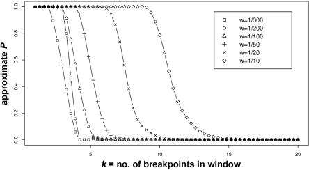
To illustrate how this approximation of the P value performs, in figure 2, we plot the calculated P values against different numbers of breakpoints k, while examining the effect of different window sizes w. We used the following assumptions: the total number of breakpoints is N=50, k∈{1…20}, and w∈{ 1/300, 1/200, 1/100, 1/50, 1/20, 1/10}. (Thus, w is normalized as the number of markers in the interval divided by the total number of markers on the chromosome.)

Figure 2. .

The tail probability P(S_w⩾k) for different numbers of breakpoints k (0⩽k⩽20) and different window sizes w. S_w is the maximum number of breakpoints in a window of length w. The total number of breakpoints in the region is N=50.

Since the computation of P values in equation (4) depends on the size of the interval w and since the size w=|I_max| of the interval I_max (found either by the Max or LR method) might not be the optimal length (e.g., because of underestimation of the length of the TSG), we also examine intervals overlapping I_max but of slightly different lengths and then compute a P value as before. From the resulting P values, we choose the smallest (most significant) value to measure the statistical significance. To account for the fact that multiple window sizes have been tested, we apply a conservative Bonferroni adjustment for the P values (we multiply the P values by the number of window sizes, and we use windows with lengths of up to 10 markers in the analysis of both simulated and real data).

Results

We applied our method to both simulated data and real data. Below, we describe the data sources, data qualities, and computed results, and we have relegated all the details to the appendix (online only).

Simulated Data

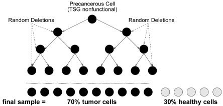
We simulated data according to the generative process that was described above. The simulation works on a growing population of cells, starting with an individual normal cell whose genome contains a single TSG at a known fixed position. As the simulation proceeds, it introduces breakpoints at different positions in the genome, each occurring as a Poisson process with rate parameter μ. At each of these breakpoints, the simulation also postulates a deletion with length distributed as an exponential random variable with parameter λ. Once, in some cell in the population, both copies of the TSG become nonfunctional (either by homozygous deletion or hemizygous deletion in the presence of other mutations), the resulting precancerous cell in the simulation starts to multiply indefinitely. Over time, the new progenitor cells also incur other independent “collateral damages” (i.e., deletions). Finally, the simulator randomly samples the population for tumor cells, mimicking the microdissection process used by a physician and, thus, assuming that the collected sample exhibits a composition of different tumor cells and some normal cells as well. In our simulations, we assumed that even the normal cells have some random deletions, whereas the different tumor cells all come from the same ancestral precancerous cell (fig. 3).

Figure 3. .

Depiction of the simulation process described in the text. A single precancerous cell (both copies of the TSG are nonfunctional) starts multiplying indefinitely. Over time, the new progenitor cells also incur other independent damage (i.e., deletions). The tumor sample that we collected comprised different tumor cells and some normal cells.

In all our simulations, we fixed the parameters, as listed below.

• N=50=number of diseased individuals.

• G=100 Mb = length of the chromosome.

• P=10,000 or P=5,000=total number of probes (with the implication of average resolutions of 10 kb and 20 kb, respectively).

• C=100=total number of cells per tumor sample, with 70% tumor cells and 30% normal cells.

• μG=2=mean number of breakpoints per cell. (This value corresponds to the background deletions that occur after the TSG becomes nonfunctional.)

•  1/λ=50 kb = mean length of a deletion.

• TSG =[10.0 Mb,10.1 Mb]. (TSG is represented by an interval starting at 10.0 Mb and has a length of 100 kb.)

To the resulting copy numbers, we added an independent Gaussian noise, ∼N(0,0.1²). The simulated data were segmented using the publicly available software described by Daruwala et al.² (NYU Versatile MAP Segmenter). A segment was called “deleted” if of the segmental:mean ratio (test:normal) for that segment was less than a threshold value of .

Table 1 shows the different simulated scenarios we used. They all share the same set of parameters as described above, with an additional complexity to reflect differences in the composition of the starting population: some samples are assumed to be diseased because of mutations in the TSG (p_homozygous+p_hemizygous), and some samples are sporadic (p_sporadic). Among the samples with mutations in the TSG, some have only homozygous deletions (p_homozygous), and some have only hemizygous deletion of the TSG (p_hemizygous). Furthermore, the sporadic samples are assumed not to have deletions in the TSG under investigation; that is, they have only background deletions.

Table 1. .

Six Simulated Models^[Note]

	Percentage of Sample
Model	phomozygous	phemizygous	psporadic
1	100	0	0
2	50	50	0
3	0	100	0
4	50	0	50
5	25	25	50
6	0	50	50

Note.— p_homozygous represents the percentage of samples in the data set with homozygous deletions, p_hemizygous is the percentage of samples with hemizygous deletions, and p_sporadic is the proportion of samples with no deletion in the TSG under investigation (randomly diseased).

Performance Measure

The performance of our method was evaluated by the Jaccard measure of overlap between the estimated position of the TSG and the real position used in the simulation. Note that, if E is the estimated interval and T is the true one, then the Jaccard measure is defined simply as

where |E∩T| is the length of the interval common to both—that is, the interval E∩T.

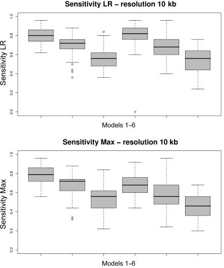
We also tested the capacity of the inferred TSG as a possible biomarker for cancer detection or classification. More precisely, we measured, for a postulated TSG, its sensitivity, which is defined as the percentage of diseased samples that have the estimated TSG deleted. For models 4–6, which also contain sporadic samples, we considered, in our calculation of sensitivity, only the more meaningful situations, consisting only of samples that are diseased because of mutations in the TSG under investigation.

Table 2 presents our results, with a summary of overlap and sensitivity measures for each of the six models outlined above and for the two marker resolutions simulated, 10 kb and 20 kb. The numbers that appear in the table are, after averaging over 50 data sets, simulated under the corresponding models. In all cases, the estimated P value is very small (<.001).

Table 2. .

Overlap between True Location and Estimated Location of the TSG and the Resulting Sensitivity for the Six Simulated Models^[Note]

	Jaccard Measure		Sensitivity
Average Intermarker Distance (kb) and Model	LR	Max	LR	Max
10:
1	.82 ± .11	.72 ± .23	.80 ± .08	.79 ± .10
2	.84 ± .12	.67 ± .24	.69 ± .10	.67 ± .13
3	.84 ± .10	.62 ± .30	.56 ± .11	.54 ± .13
4	.74 ± .15	.23 ± .19	.80 ± .14	.69 ± .12
5	.73 ± .16	.33 ± .25	.69 ± .12	.59 ± .16
6	.74 ± .17	.26 ± .25	.54 ± .12	.46 ± .12
20:
1	.70 ± .15	.44 ± .27	.59 ± .16	.56 ± .16
2	.70 ± .19	.38 ± .30	.46 ± .14	.43 ± .15
3	.68 ± .20	.43 ± .30	.38 ± .14	.34 ± .16
4	.60 ± .21	.25 ± .21	.60 ± .18	.55 ± .15
5	.65 ± .20	.24 ± .22	.46 ± .15	.40 ± .14
6	.58 ± .28	.27 ± .28	.37 ± .15	.33 ± .14

Note.— LR and Max refer to the two methods used to estimate the location of the TSG.

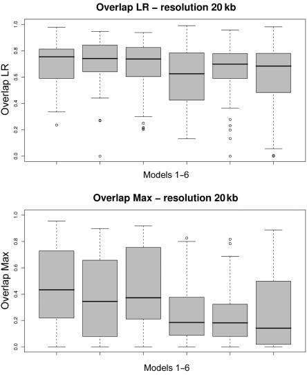
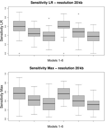
To present a better understanding of the entire distribution of scores, we also plotted box plots for the Jaccard measure and for the sensitivity measure for all the simulated scenarios (see figs. 4–7).

Figure 4. .

Box plots of the Jaccard measure of overlap for each of the six models (table 1). Fifty data sets are simulated according to each model, and the distribution of the resulting 50 overlap measures is depicted in each box plot. Average intermarker distance is 10 kb. A, LR. B, Max.

Figure 5. .

Box plots of the sensitivity measure for each of the six models (table 1). Fifty data sets are simulated according to each model, and the distribution of the resulting 50 sensitivity measures is depicted in each box plot. Average intermarker distance is 10 kb. A, LR. B, Max.

Figure 6. .

Box plots of the Jaccard measure of overlap for each of the six models (table 1). Fifty data sets are simulated according to each model, and the distribution of the resulting 50 overlap measures is depicted in each box plot. Average intermarker distance is 20 kb. A, LR. B, Max.

Figure 7. .

Box plots of the sensitivity measure for each of the six models (table 1). Fifty data sets are simulated according to each model, and the distribution of the resulting 50 sensitivity measures is depicted in each box plot. Average intermarker distance is 20 kb. A, LR. B, Max.

Real Data

Real data from patients with cancer or from cancer cell lines, when examined with an available array technology, may contain other sources of error that may be correlated or may be nonstationary in a complicated manner that can never be modeled in the simulation; effects difficult to model include degradation of genomic DNA, base-composition–dependent PCR amplification in complexity reduction, presence of hypermutational regions, incorrect probes resulting from errors in reference genome assembly, contamination, crosshybridization, and myriad others. Consequently, we cannot obtain full confidence in our methodologies, even though the results of the analysis of the simulated data were found to be very encouraging and even though the analysis showed that, in those ideal conditions underlying the simulation, our algorithm was able to detect, with high accuracy and confidence, the location of the simulated TSG.

In this section, we inspect the results of our method when applied to a real data set for lung cancer, which was originally published by Zhao et al.⁵ Seventy primary human lung-carcinoma specimens were used in our analysis. For each sample, copy-number changes at ∼115,000 SNP loci throughout the genome were measured and recorded. We used an unpublished Affy normalization and summarization software (T. S. Anantharaman, S. Paxia, and B.M., unpublished data) to convert the raw data into genotypic copy-number values. Next, as for the simulated data, we applied the segmentation algorithm² to the raw signal ratio (test:normal) data and obtained a partition of the data into segments of probes with the same estimated mean. Since the previous steps were found to average out the random noises across groups of probe sets and neighboring probes, variance parameters were quite low and were discarded from further analysis. 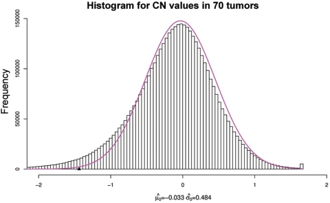For this data set, we next determined that a chromosomal segment could be treated as deleted if the segment had an inferred ratio less than a threshold value of −1.0. Figure 8 depicts the histogram for the ratio values for all SNPs in all 70 tumors, together with an empirical null density fitted to the histogram . The overall threshold is defined as . (The appendix [online only] provides further details about the computation of this cutoff threshold.)

Figure 8. .

The histogram for the ratio values for all SNPs in all 70 tumors, together with an empirical null density fitted to the histogram: .

The significant regions (genomewide significance level <.01) are presented in table 3. The intervals reported were computed using the Max method. Most of the detected regions have been reported elsewhere as deleted in lung cancer (e.g., 5q21 and 14q11). Most significantly, some of the found intervals overlap some good candidate genes that may play a role in lung cancer (e.g., MAGI3, HDAC11, and PLCB1). Also, Zhao et al.⁵ found, for the first time, that regions 3q25 and 9p23 were homozygously deleted.

Table 3. .

Significant Deleted Regions in the Lung Cancer Data Set

Chromosome	Exact Interval (Mb)	Commentsa
1p13.2	113.76–113.77	MAGI3 maps to this regionb
3p25.1	13.51–13.56	HDAC11 maps to this regionc
3q25.1	151.16–151.16	Homozygous deletions in this region have been found using this data set5
4q34.1	173.46–173.46	Deletions in this region have been reported in lung cancer8,9
5q14.1	79.16–79.18
5q21.3	106.95–107.0	This region is known to be frequently deleted in lung cancer10
6q14.1	78.50–79.02
7p15.3	20.48–20.49
9p23	10.02–10.05	Homozygous deletions in this regiond have been found using this data set5
9p21	32.85–32.85	Deletions in this region have been reported in lung cancer
10p13	17.17–17.20
10q24.1	97.83–97.94	BLNK maps to this regione
11p15.4	4.9–5.0	Deletions in this region have been found in several cancers11
12q14	66.28–66.29
14q11.2	20–20.1	Loss of heterozygosity in this regionf has been reported in lung cancer12
16q24	82.8–82.8	CDH13, known TSG, is deleted in lung cancer
17q21	39.5–39.6	HDAC5 maps to this regiong
19p13.3	.34–2	LKB1 is deleted in lung cancer13
20p12	8.7–8.8	PLCB1 maps to this regionh
21q21.2	23.27–23.38	This region has been found deleted in lung cancer15

^aFor more information, see the National Center for Biotechnology Information Human Genome Resources Web site.

^bPTEN/MMAC and MAGI3 cooperate to modulate the kinase activity of AKT/PKB involved in the inhibition of apoptosis.⁶

^cFrequent allelic losses have been reported in this region in lung and other solid tumors. Also, in vitro studies suggest that this region is able to suppress growth of tumor cells.⁷

^dThis region is upstream of PTPRD (protein tyrosine phophatase, receptor type D), the gene currently being investigated for its potential implications in lung cancer.⁵

^eBLNK is a putative TSG.

^fAPEX1 maps to this region; this gene is implicated in the DNA repair mechanism and in control of cell growth.

^gHDAC5 plays a critical role in transcriptional regulation, cell-cycle progression, and developmental events.

^hThis gene is important in the control of cell growth; it may be of interest in cancer.¹⁴

Discussion

The focus of this work has been a novel statistical method and its application to the problem of estimating the location of TSGs from arrayCGH data characterizing segmental deletions in cancer genomes. The underlying algorithm computes a multipoint score for all intervals of consecutive probes. The computed score measures how likely it is for a particular genomic interval to be a TSG implicated in the disease. We propose two ways to estimate the location, the LR method and the Max method. In our experience, both methods perform well, with the LR method being more accurate than the Max method in the simulation experiments, especially when the marker density is relatively high (i.e., ⩾100,000 probes spanning the human genome). However, with the real data, we found that the Max method gives better intervals, because of the increased noise.

We evaluated the efficacy of our method by applying it to both simulated data and real data, and we concluded that the results are significant. In the ideal conditions, as in our simulations, our estimation method seems to perform exceedingly well. In particular, with an average intermarker distance of 10–20 kb, the overlap between the estimated position and the true position of the TSG is >50%. Although the simulations are only an attempt to approximate the real data, the results obtained show that our method is reliable in pinpointing the location of putative TSGs. In addition, we also applied our method to a real data set for lung cancer. We obtained many regions that were reported elsewhere as deleted in lung cancer. Most significantly, the intervals within the regions 3p25, 16q24, 19p13, and 20p12 overlap some good candidate genes (HDAC11, CDH13, LKB1, and PLCB1, respectively) that could play an important role in lung cancer. Several other regions have also been known to harbor deletions in patients with lung cancer. In addition, we detected a few regions, unreported elsewhere, that warrant more-detailed examination to understand their relation to lung cancer—for example, 6q14 and 7p15.

We note that, in comparative experimental settings such as those used by arrayCGH, one needs to keep track of the meaning of “normal genomes,” since there are at least three kinds of “normal” genomes involved in this analysis—namely, the normal genome (or genomes) used in designing the arrayCGH (or SNP) chips, the genomes from a population with similar distribution of polymorphisms (both SNPs and copy-number polymorphisms [CNPs]) as the patient under study, and, finally, the genome from a normal cell in the same patient. The simplest situation, in terms of statistical analysis, is when the normal genome is the one from a normal cell from the same patient; this is at the basis of the analysis we presented here. The other information can be augmented in preprocessing or postprocessing steps, when the situation differs from this simplest one. Also, our scoring functions and the algorithm can be suitably modified if it is deemed necessary that the polymorphisms in the probes and the population must be tracked. Other similar, but not insurmountable, complications would arise, if one were to also model the “field effects” in the normal genomes from the patient.

We also note that this study highlights only the application to estimating the positions of TSGs. However, the estimation for oncogenes requires only minor modifications to the score function and to the estimation method, since, for an oncogene, the mutation (i.e., amplification) is dominant and requires the entire gene to be amplified, whereas, for TSGs, the mutation is recessive, and it suffices for any functional portion of the gene to be deleted for its inactivation.

In summary, we formulated a general approach that is likely to apply to other problems in genetics if a suitable generative model and an accompanying score function can be accurately formulated; the rest of the method works out mutatis mutandis. Unlike the classic approach, normally employed in most genetics studies, the proposed approach does not employ a locus-by-locus analysis and thus does not depend on linkages between a marker and genes that harbor causative mutations. The present algorithm exploits the fact that, when genomewide high-density markers are studied, as with whole-genome arrays, one could look for the interesting genes directly by examining every plausible genomic interval delineated by a group of consecutive markers. Such an interval-based analysis is more informative and allows assignment of significance values to estimated intervals with use of scan statistics. We note that there have been other uses of scan statistics for genetics in different contexts, such as the work of Hoh and Ott.¹⁶

We also note that many variants of our method can be further enriched by augmenting other auxiliary information to the interval: underlying base compositions (e.g., GC content, Gibbs-free energy, and codon bias) in the genomic interval, known polymorphisms (e.g., SNPs and CNPs), genes and regulatory elements, structures of haplotype blocks, recombination hot spots, etc. Note, however, that, at present, in the absence of reliable and complete statistical understanding of these variables, it is safe to work only with uninformative and simple priors of the kind we have already incorporated in our algorithm.

Nonetheless, the utility of our algorithm will most likely be first validated with the simplest forms of arrayCGH data and in the context of cancer, an area currently under intense study. We will gain more confidence as these methods are used for bigger data sets, for larger number of patients, and for many different cancers. There are few competing methods that bear some minor resemblance to our algorithm. For instance, the STAC method (Significance Testing for Aberrant Copy-Number [STAC] Web site) also finds gene intervals from arrayCGH data, but it does not employ any generative model to compute a score to be optimized, nor does it compute a statistical significance on the basis of such a model. (It uses a permutation approach to create a null-hypothesis model). A detailed comparison will indicate how much statistical power is gained when a more faithful but parsimonious generative model is used.

We recognize that a lot more remains to be done to completely realize all the potential of the proposed analysis. There may be more-subtle correlations between the intervals we detect, and such correlations (or anticorrelations) may hint at subtle mechanisms in play in cancer progression. If various regions of a polyclonal tumor can be analyzed separately, the distribution of important intervals may reveal many more details of the disease. There may be a critical need to stratify the patients into subgroups and to analyze them separately to detect more-subtle patterns. Once an important interval is detected (e.g., corresponding to a putative TSG), one may wish to understand how the deleted intervals affecting the genes are spatially distributed. Such higher-order patterns and motifs may paint a better picture about many varied genomic mechanisms responsible for the initiation and development of a cancer.

Appendix

Proof of the Lemma

Suppose we have the following generative process: breakpoints occur along the genome according to a Poisson process with rate μ. At each breakpoint, there is a deletion with length distributed as an exponential random variable with parameter λ. The direction (left or right) of the deletion is decided by a Bernoulli trial (p=0.5).

Lemma 1.—According to this process, the probability that an interval I=[a,b] is deleted is

Proof: Given an interval [a,b], it is easier to compute the following probability

We know that [a,b]∩Del=φ happens if and only if there is no breakpoint in [a,b] and each deleted interval starting from a breakpoint in [0,a] does not overlap with [a,b] and each deleted interval starting from a breakpoint in [b,G] does not overlap with [a,b].

Let P₁ be the probability of the first event, P₂ be that of the second, and P₃ be that of the last event. P₁, the probability of no breakpoint in [a,b], is just

The second probability, P₂, can be written as

We can now compute the terms in this sum. The first term is P(nobreakpointin [0,a])=e^-μa. For the second term, P(1 breakpointin [0,a])×P(deletedinterval∩[a,b]=φ), we have first P(1 breakpointin [0,a])=μae^-μa and P(deletedinterval∩[a,b]=φ), which is more complicated.

Suppose we divide the interval [0,a] into many small intervals [x_i,x_i+1] for i∈{0,…,n}. Then

Let us now compute the probability of no overlap caused by the deletion at x∈[x_i,x_i+1].

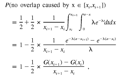where

Therefore,

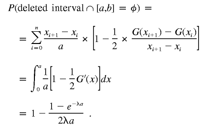So the second term in P₂ is

For the third term, P(twobreakpointsin [0,a])×P(deletedintervals∩[a,b]=φ), we have first

and

Now,

by simple probability computations.

We have already computed

and

where

Therefore,

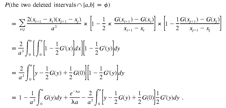Integrating by parts, we obtain

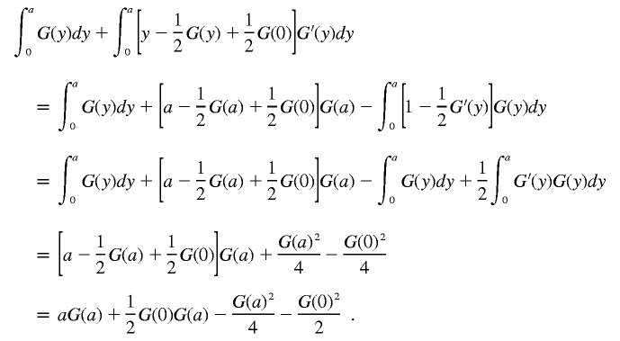Hence,

Since G(a)= 1/λ and G(0)= e-λa/λ, we obtain

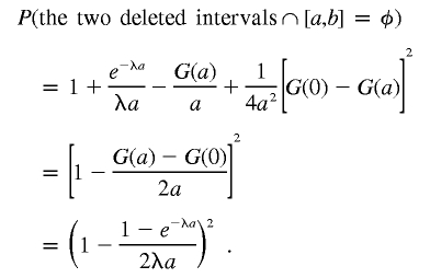We can now say that the third term in P₂ is

Finally, we obtain

Hence,

The last probability we need to compute is P₃, the probability that each deleted interval starting from a breakpoint in [b,G] does not overlap with [a,b]. Through computations similar to those for P₂, we can show that

The final formula is

therefore,

Copy-Number Distribution for Individual Samples

Our rule for calling a segment “deleted” is that the of the segmental:mean ratio (test:normal) for that segment be less than a certain threshold. To determine this threshold, we proceed as follows. For each sample in the data set, we fit an empirical null density to the histogram of copy numbers; thus, we obtain the null density . We then define the threshold for each individual sample as , and the average of these values is the overall cutoff we use. By this method, we obtain c=-1.0.

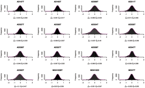
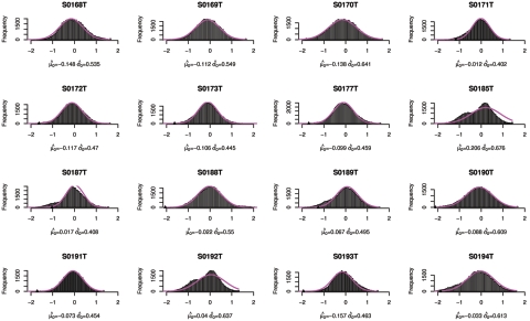
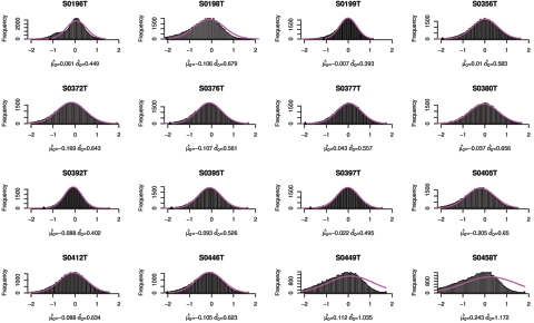
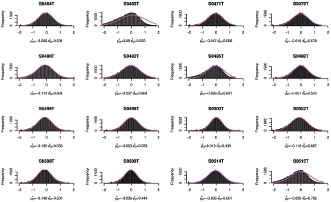
In figures 9–13, we show, for each sample, the histogram of copy numbers together with the empirical null density fitted to the data. Below each plot are the estimated (mean) and (SD) for the empirical null density.

Figure 9. .

Copy-number histogram for individual samples (samples 1–16). Overlaid is the fitted empirical null density .

Figure 10. .

Copy-number histogram for individual samples (samples 17–32). Overlaid is the fitted empirical null density .

Figure 11. .

Copy-number histogram for individual samples (samples 33–48). Overlaid is the fitted empirical null density .

Figure 12. .

Copy-number histogram for individual samples (samples 49–64). Overlaid is the fitted empirical null density .

Figure 13. .

Copy-number histogram for individual samples (samples 65–70). Overlaid is the fitted empirical null density .

References

- 1.Knudson AG (1971) Mutation and cancer: statistical study of retinoblastoma. Proc Natl Acad Sci USA 68:820–823 10.1073/pnas.68.4.820 [DOI] [PMC free article] [PubMed] [Google Scholar]
- 2.Daruwala RS, Rudra A, Ostrer H, Lucito R, Wigler M, Mishra B (2004) A versatile statistical analysis algorithm to detect genome copy number variation. Proc Natl Acad Sci USA 101:16292–16297 10.1073/pnas.0407247101 [DOI] [PMC free article] [PubMed] [Google Scholar]
- 3.Glaz J, Naus J, Wallenstein S (2001) Scan statistics. Springer-Verlag, New York [Google Scholar]
- 4.Wallenstein S, Neff N (1987) An approximation for the distribution of the scan statistic. Stat Med 6:197–207 [DOI] [PubMed] [Google Scholar]
- 5.Zhao X, Weir BA, LaFramboise T, Lin M, Beroukhim R, Garraway L, Beheshti J, Lee JC, Naoki K, Richards WG, Sugarbaker D, Chen F, Rubin MA, Janne PA, Girard L, Minna J, Christiani D, Li C, Sellers WR, Meyerson M (2005) Homozygous deletions and chromosome amplifications in human lung carcinomas revealed by single nucleotide polymorphism array analysis. Cancer Res 65:5561–5570 10.1158/0008-5472.CAN-04-4603 [DOI] [PubMed] [Google Scholar]
- 6.Wu Y, Dowbenko D, Spencer S, Laura R, Lee J, Gu Q, Lasky LA (2000) Interaction of the tumor suppressor PTEN/MMAC with a PDZ domain of MAGI3, a novel membrane-associated guanylate kinase. J Biol Chem 275:21477–21485 10.1074/jbc.M909741199 [DOI] [PubMed] [Google Scholar]
- 7.Rimessi P, Gualandi F, Morelli C, Trabanelli C, Wu Q, Possati L, Montesi M, Barrett JC, Barbanti-Brodano G (1994) Transfer of human chromosome 3 to ovarian cancer cell lines identifies three region on 3p involved in ovarian cancer. Oncogene 9:3467–3474 [PubMed] [Google Scholar]
- 8.Shivapurkar N, Virmani AK, Wistuba II, Milchgrub S, Mackay B, Minna JD, Gazdar AF (1999) Deletions of chromosome 4 at multiple sites are frequent in malignant mesothelioma and small cell lung carcinoma. Clin Cancer Res 5:17–23 [PubMed] [Google Scholar]
- 9.Tseng RC, Chang JW, Hsien FJ, Chang YH, Hsiao CF, Chen JT, Chen CY, Jou YS, Wang YC (2005) Genomewide loss of heterozygosity and its clinical associations in non small cell lung cancer. Int J Cancer 117:241–247 10.1002/ijc.21178 [DOI] [PubMed] [Google Scholar]
- 10.Hosoe S, Ueno K, Shigedo Y, Tachibana I, Osaki T, Kumagai T, Tanio Y, Kawase I, Nakamura Y, Kishimoto T (1994) A frequent deletion of chromosome 5q21 in advanced small cell and non-small cell carcinoma of the lung. Cancer Res 54:1787–1790 [PubMed] [Google Scholar]
- 11.Karnik P, Paris M, Williams BR, Casey G, Crowe J, Chen P (1998) Two distinct tumor suppressor loci within chromosome 11p15 implicated in breast cancer progression and metastasis. Hum Mol Genet 7:895–903 10.1093/hmg/7.5.895 [DOI] [PubMed] [Google Scholar]
- 12.Abujiang P, Mori TJ, Takahashi T, Tanaka F, Kasyu I, Hitomi S, Hiai H (1998) Loss of heterozygosity (LOH) at 17q and 14q in human lung cancers. Oncogene 17:3029–3033 10.1038/sj.onc.1202230 [DOI] [PubMed] [Google Scholar]
- 13.Sanchez-Cespedes M, Parrella P, Esteller M, Nomoto S, Trink B, Engles JM, Westra WH, Herman JG, Sidransky D (2002) Inactivation of LKB1/STK11 is a common event in adenocarcinomas of the lung. Cancer Res 62:3659–3662 [PubMed] [Google Scholar]
- 14.Peruzzi D, Aluigi M, Manzoli L, Billi AM, Di Giorgio FP, Morleo M, Martelli AM, Cocco L (2002) Molecular characterization of the human PLC β1 gene. Biochim Biophys Acta 1584:46–54 [DOI] [PubMed] [Google Scholar]
- 15.Lee EB, Park TI, Park SH, Park JY (2003) Loss of heterozygosity on the long arm of chromosome 21 in non-small cell lung cancer. Ann Thorac Surg 75:1597–1600 10.1016/S0003-4975(02)04902-0 [DOI] [PubMed] [Google Scholar]
- 16.Hoh J, Ott J (2000) Scan statistics to scan markers for susceptibility genes. Proc Natl Acad Sci USA 97:9615–9617 10.1073/pnas.170179197 [DOI] [PMC free article] [PubMed] [Google Scholar]