Multipass Membrane Protein Structure Prediction Using Rosetta

Abstract

We describe the adaptation of the Rosetta de novo structure prediction method for prediction of helical transmembrane protein structures. The membrane environment is modeled by embedding the protein chain into a model membrane represented by parallel planes defining hydrophobic, interface, and polar membrane layers for each energy evaluation. The optimal embedding is determined by maximizing the exposure of surface hydrophobic residues within the membrane and minimizing hydrophobic exposure outside of the membrane. Protein conformations are built up using the Rosetta fragment assembly method and evaluated using a new membrane-specific version of the Rosetta low-resolution energy function in which residue–residue and residue–environment interactions are functions of the membrane layer in addition to amino acid identity, distance, and density. We find that lower energy and more native-like structures are achieved by sequential addition of helices to a growing chain, which may mimic some aspects of helical protein biogenesis after translocation, rather than folding the whole chain simultaneously as in the Rosetta soluble protein prediction method. In tests on 12 membrane proteins for which the structure is known, between 51 and 145 residues were predicted with root-mean-square deviation <4Å from the native structure.

INTRODUCTION

Alpha helical transmembrane (TM) proteins have a key role in biological processes, such as signal transduction and selective transport of ions, cations, and water. The biological significance of the helical TM proteins is highlighted by the fact that >50% of current drugs in use target membrane proteins.¹ Helical TM proteins are predicted to encode 20–30% of all open reading frames of known genomes^2-4; however, currently, all types of membrane proteins represent only about 0.6% (168⁵ of 28,000) of solved protein structures in the Protein Data Bank (PDB).⁶ Difficulties in producing sufficient quantities of properly folded protein and in obtaining high-resolution crystals have proven to be very significant obstacles to determine atomic level structures of membrane proteins. Recently, there has been significant progress in de novo structure prediction of soluble proteins,^7-9 offering some hope that structure prediction methodology may be able to contribute to understanding membrane protein structure.

Statistical analysis of available α-helical membrane protein structures by many research groups has yielded useful information about amino acid environmental preferences within the hydrophobic, interface, and polar layers of the membrane. In 1989, Rees et al.¹⁰ observed that membrane-exposed residues on average are more hydrophobic than buried residues in the hydrophobic layer of the membrane in the photosynthetic reaction center structure. More recently, analysis of amino acid distributions in helical TM protein structures has shown that large hydrophobic amino acids, such as leucine, isoleucine, valine, and phenylalanine indeed favor the lipid-exposed environment versus the protein-buried environment^11-13 and that small side-chain amino acids, such as glycine, alanine, serine, and threonine favor helix–helix interfaces, suggesting that these amino acids have a critical role in forming specific helix–helix interactions in the membrane proteins.^11,14-17 Analysis of residue–residue interfacial pairwise propensities in helical TM proteins revealed that polar and cation-pi interactions are more frequent in helical TM proteins than in water-soluble proteins¹⁸ and that the majority of TM helices in the helical TM proteins have interhelical side-chain–side-chain hydrogen bonds which induce tighter packing of the helices.¹⁹ In addition, a role for polar residues in mediating helix–helix association in the hydrophobic layer of the membrane has been shown experimentally.^20-23

Herein, we report the adaptation of the Rosetta de novo structure prediction method^24-26 to membrane protein structure prediction. Both the fragment-based structure generation method and the low-resolution scoring function have been adapted for the anisotropic membrane environment. The new method can predict significant portions of each of 12 tested proteins with root-mean-square deviation (RMSD) from the native structure <4Å.

MATERIALS AND METHODS

Membrane Layer Scoring Function

The membrane is modeled using two parallel planes separated by 60 Å. Between two planes the energy computed from a sum of terms were analogous to those used in the Rosetta low-resolution soluble protein prediction method^24-26:

$$E_{\mathit{total}}=E_{\mathit{env}}+E_{\mathit{pair}}+E_{\mathit{clash}}+E_{\mathit{density}}+E_{\mathit{strand}},$$

where E_env and E_pair model residue–environment and residue–residue interactions and were derived from a membrane protein dataset as described below, E_clash penalizes steric overlaps, E_density favors packing density characteristic of membrane protein, and E_strand favors strand pairings.

The amino acid environment, pair and density terms were calculated from a set of 28 helical TM protein structures found in the PDB (see Table I). Multiple sequence alignment (MSA) information from homologous proteins with ≥30% sequence identity to the parent structure sequence was used to increase the number of observations for E_env and E_pair, which was particularly important for amino acids with a low number of counts. For each position, the contribution of an amino acid to the counts for the corresponding structural environment is simply the frequency of the amino acid in the MSA. For example, if alanine was 70% conserved at a particular residue in a structure, it contributed 0.7 counts to total statistics for the relevant membrane environment.

TABLE I.

Membrane Proteins Used in Statistical Analysis

No.	Protein name	PDB code	Resolution (Å)	Total number of residues	Chains/segments	Contribution to total statistics (%)
1	Rhodopsin	1F88	2.8	338		2
2	Bacteriorhodopsin	1C3W	1.5	222		1
3	Multidrug efflux transporter AcrB	1IWG	3.5	1,006		7
4	Halorhodopsin	1E12	1.8	239		2
5	Lactose permease transporter	1PV6	3.5	417		3
6	Aquaporin water channel AQP1	1J4N	2.2	249		2
7	Glycerol facilitator channel GlpF	1FX8	2.2	254		2
8	Protein-conducting channel SecYEβ	1RHZ	3.5	529	A, B, C	3
9	Glycerol-3-phosphate transporter GlpT	1PW4	3.3	434		3
10	Lipid transporter MsbA	1PF4	3.8	1,040		3
11	Vitamin B12 transporter BtuCD	1L7V	3.2	1,074	A, C	3
12	Calcium ATPase	1EUL	2.6	994		6
13	Photosynthetic reaction center	1PRC	2.3	1,186	C, H, L, M	8
14	Fumerate reductase complex	1QLA	2.2	986	B, C	3
15	Formate dehydrogenase-N	1KQF	1.6	1,515	B, C	3
16	Succinate dehydrogenase	1NEK	2.6	1,068	A, B, C, D	7
17	Nitrate reductase NarGHI	1Q16	1.9	732	B, C	5
18	Mitochondrial ADP/ATP carrier	1OKC	2.2	292		2
19	Cytochrome C oxidase aa3	1OCC	2.8	1,780	A, B, C, D, E, F, G, H, I, K, L, M	12
20	Cytochrome bc1 complex	1BGY	3.0	1,842	A, B, C, D, E, F, G, I, J	12
21	Potassium channel KcsA	1K4C	2.0	412		1
22	Potassium channel MthK	1LNQ	3.3	1,204		2
23	Potassium channel KvAP	1ORQ	3.2	372	S5-P-S6 segments only	1
24	Potassium channel KirBac1.1	1P7B	3.7	1,032		2
25	Mechanosensitive channel McsL	1MSL	3.5	545		1
26	H+/Cl− exchange transporter CIC	1KPL	3.0	881		3
27	Potassium channel KvAP	1ORS	1.9	132	S1-S4 segments only	1
28	Ammonia channel AmtB	1U77	1.4	1,116		2

E_env

The membrane environment was divided into horizontal layers approximately corresponding to the water-exposed, polar, interface, and hydrophobic layers of the membrane as described by White and Wimley²⁷ (Fig. 1). The hydrophobic layer was divided into outer and inner sublayers because preliminary analysis showed significant difference in environment profiles for tyrosine (see Results) and tryptophan (data not shown) between these sublayers. The membrane normal was defined as a vector between the average position of C^α atoms of the TM helices terminal residues on the intracellular $\left({\mathrm{C}}_{\mathrm{int}}^{\alpha }\right)$ and extracellular $\left({\mathrm{C}}_{\mathrm{ext}}^{\alpha }\right)$ sides of the membrane and the center of the membrane was taken to be halfway between ${\mathrm{C}}_{\mathrm{int}}^{\alpha }$ and ${\mathrm{C}}_{\mathrm{ext}}^{\alpha }$. Planes perpendicular to the membrane normal and 30 Å from the center of the membrane were taken to represent a 60-Å-thick membrane bilayer. The bilayer and surrounding solvent region were divided into five layers as shown in Figure 1. Residues were classified into eight burial states based on the number of residue centroids within 10 Å. The details of the layer and burial bins are described in Table II. Thus, 8 burial × 5 layer = 40 possible burial/layer states were defined for each residue. The membrane environment score was defined as:

$$E_{\mathit{env}}=\sum _i-\ln \left(\frac{P({\mathit{aa}}_i\mid L,B)}{P\left({\mathit{aa}}_i\right)}\right)$$

where i is a residue index, P(aa_i|L,B) is the frequency of amino acid type aa_i in a layer/burial (L,B) state and P(aa_i) is the frequency of amino acid type aa_i in all layer/burial states.

Fig. 1.

Membrane layer definition. The lowest energy embedding of the fumarate reductase complex structure (PDB 1QLA) found using the method discussed in the text is colored as follows: “water-exposed” layer—dark blue; “polar” layer—light green; “interface” layer—green; “outer hydrophobic” layer—yellow; and “inner hydrophobic” layer—red.

TABLE II.

Bins Used in Membrane Sore Function

Function	Variable	Bins
Eenv	Membrane layer	<0, 0–12, 12–18, 18–24, 24–30 Å
Eenv	Number of neighbors	0–9, 10–12, 13–15, 16–18, 19–21, 22–24, 25–27, >27
Epair	Residue–residue centroid distance	0–5, 5–7.5, 7.5–10, 10–12, >12 Å

E_pair

For analysis of amino acid pair propensities, the membrane plane was divided into two layers—polar and hydrophobic. The polar layer included the water-exposed, polar, and interface layers, and the hydrophobic layer included the outer and inner hydrophobic layers defined as for the analysis of amino acid membrane environment propensities (see above). Pair propensities were calculated for five residue–residue centroid distance bins listed in Table II. E_pair was defined as:

$$E_{\mathit{pair}}=\sum _i\sum _{i<j}-\ln \left(\frac{P({\mathit{aa}}_i,{\mathit{aa}}_j\mid d_{\mathit{ij}},L)}{P{({\mathit{aa}}_i\mid d_{\mathit{ij}},L)}^{\ast }P({\mathit{aa}}_j\mid d_{\mathit{ij}},L)}\right)$$

where $P({\mathit{aa}}_i,{\mathit{aa}}_j\mid d_{\mathit{ij}},L)=\frac{N({\mathit{aa}}_i,{\mathit{aa}}_j\mid d_{\mathit{ij}},L)+M\ast \frac{N({\mathit{aa}}_i,{\mathit{aa}}_j)}{N_{\mathit{tot}}}}{N(d_{\mathit{ij}},L)+M}$, i and j are residue indices, P(aa_i | d_ij,L) is the frequency of amino acid type aa_i within distance bin d_ij in layer L, P(aa_j | d_ij,L) is the frequency of amino acid type aa_j within distance bin d_ij in layer L, N(aa_i,aa_j | d_ij,L) is the number of counts of pair of amino acid types aa_i and aa_j within distance bin d_ij in layer L, N(aa_i,aa_j) is the total number of counts of pair of amino acid types aa_i and aa_j in all layers and all distance bins, N(d_ij,L) is the total number of amino acids within distance bin d_ij in layer L, N_tot is the total number of amino acids in all layers and all distance bins, and M is the number of pseudo counts which was equal to 100. E_pair values were capped between −0.95 and 0.75 with the exception of cysteine–cysteine pairs, in order to be in a range of E_pair values observed for water-soluble proteins.

E_density

For analysis of residue density profile, the membrane plane was divided into two layers—polar and hydrophobic—defined as for the analysis of amino acid pair propensities (see above). Analysis of residue density in the representative set of water-soluble α-helical proteins (see Table III) was also performed. As in the standard Rosetta method, two density terms, one based on a 6 Å sphere and the other one on a 12 Å sphere around each residue centroid were used to capture both close-range residue packing and overall protein density.

TABLE III.

Water-Soluble Proteins Used in Residue Density Analysis

No.	Protein name	PDB code	Resolution (Å)	Number of helices	Total number of residues
1	Hydrolase, transferase	1VJ7	2.1	13	326
2	Mam-Mhc complex (chain H)	1R5I	2.6	7	214
3	YcfC-like protein	1QZ4	2.0	8	213
4	Set domain of LSMT	1P0Y	2.6	9	430
5	pH-beach domain of neurobeachin	1MI1	2.9	9	414
6	Guanine nucleotide region of intersectin	1KI1	2.3	7	342
7	Class I α1,2-mannosidase	1F03	1.8	14	455
8	Guanylate binding protein-1	1F5N	1.7	12	570
9	Glycerol-3-phosphate dehydrogenase	1EVY	1.8	12	346
10	Deoxyribodipyrimidine photolyase	1DNP	2.3	14	469

Fragment selection

For each TM protein tested, structure fragments were generated as described for the standard Rosetta method by Rohl et al.,²⁴ except that only the SAM-T99²⁸ secondary structure prediction method was used during fragments selection procedure [the other two secondary structure prediction methods used by standard Rosetta—Psipred²⁹ and JUFO³⁰—poorly predicted the majority of α-helical TM regions (data not shown), which is not surprising because they were trained for soluble protein secondary structure prediction].

TM region prediction

We used TMHMM,^31,32 TMPred,³³ MEMSAT2,³⁴ and HMMTOP^35,36 to define positions of N- and C-terminal residues of each of the TM helices in all TM proteins tested, which were used to approximate the membrane normal vector (see its definition in E_env above) needed for our scoring function during each step of TM protein folding.

RESULTS

An immediate challenge confronting membrane protein structure prediction is the anisotropy of the surrounding environment. To model the portion of the protein within the membrane, we developed a representation of the membrane based on infinite parallel planes dividing the membrane into layers with distinct amino acid preferences (see below). Initial attempts at directly applying the fragment assembly method developed for soluble proteins with the membrane layer fixed in space did not lead to native-like structures. The acceptance rate was very low because a fragment insertion can result in a structure that could in principle span the membrane, but which is not oriented properly relative to the membrane plane. Rather than reject these structures, we developed a rapid method to find the lowest energy embedding of the protein in the membrane after every fragment insertion. Finally, we modified our fragment-based structure generation procedure to more efficiently produce structures that embed well in the membrane.

The following three sections describe the method: first, the search for embeddings, second, the representation of membrane environment, and third, the structure generation method. In the final section we describe the prediction of membrane protein structures using the method.

Search for Embeddings

Because the energy of a structure depends on how it sits in membrane layers, we search for the optimal embedding after every trial move. There are three components of the score that depend on the embedding: 1. a penalty for predicted TM helices that do not span the membrane; 2. a penalty for nonhelical backbone torsional angles in the core of the membrane; 3. the environment and pair scores, which change depending on the layer of the membrane.

The membrane is described by a surface normal direction and a location along this normal for its center. For every configuration, an initial estimate of the embedding is made by taking the center of the membrane as the center of mass of the protein, and the normal as the average direction of the helices predicted to cross the membrane at that stage. The direction of a helix is measured as the vector between the C^α atoms at each end of the predicted spanning region. A Monte Carlo search is then performed around this initial guess, by varying the angle of the membrane normal and the position of the membrane center relative to the protein center, searching for the lowest energy embedding. This search can be done quickly, because the terms of the score that vary depend primarily on a residue's neighbors, which do not change with embedding. Finding the embedding with the lowest energy at each step recapitulates the simultaneous optimization of chain configuration and membrane orientation during membrane protein folding.

This embedding procedure was tested on 24 crystal structures, and the embedding angles were compared with those in a curated database of embeddings of protein structures.³⁷ In 21 of 24 cases, the dot product of the computed embedding vector with the embedding vectors from the database were between 0.9 and 1.0 and in three other cases between 0.8 and 0.9 (data not shown), showing that our method for inferring the placement of a membrane protein in the membrane from its structure is reasonably accurate.

Model for Membrane Environment

Residue environment interactions

Membrane environment specific amino acid propensities within and outside of the 60-Å-thick membrane bilayer model were calculated from a representative set of TM protein structures (see Materials and Methods). Membrane environment score plots for representatives of hydrophobic, small side-chain, aromatic, and polar amino acid classes are shown in Figure 2. Leucine—representative of large hydrophobic amino acids—was the most frequently observed amino acid in the membrane protein set—contributing between 8 and 16% to the total counts in the different membrane layers (see Fig. 1S in Supplementary Material, http://www.interscience.wiley.com/jpages/0887-3585/suppmat). As expected, leucine strongly prefers to be buried within the protein environment within the water-exposed layer [Fig. 2(A)]. In contrast, leucine strongly prefers to be exposed to the lipid environment within the hydrophobic layer of the membrane. Other large hydrophobic residues—isoleucine, valine, and phenylalanine—also have a similar environment profile (data not shown), in agreement with previously published reports.^10,11,14-17 Glycine has relatively weak propensity in most buried environments in the water-exposed and polar layers of the membrane [Fig. 2(B)]. In contrast, glycine strongly prefers to be in all buried environments within the hydrophobic layer of the membrane, supporting previously reported observations showing that glycine and other small side-chain amino acids are important for the helix–helix packing interactions.^11,14-17 Tyrosine strongly prefers to be within the interface layer of the membrane in most burial states [Fig. 2(C)], consistent with previous studies.^38-40 As expected, lysine strongly prefers to be exposed in water-exposed, polar, and interface layers of the membrane [Fig. 2(D)] and is disfavored in the hydrophobic layer of the membrane.

Fig. 2.

Plots of membrane environmental score profiles for representative hydrophobic, small side-chain, aromatic, and polar amino acids. x Axis: the eight-residue burial states defined in Table II shown separately for each membrane layer (layer name labeled at the top of each plot). Number 9 on the plot indicates the number of neighbors between 0 and 9, number 12 indicates the number of neighbors between 10 and 12, etc. y Axis: E_env. A: Plot of membrane environment score for leucine. B: Plot of membrane environment score for glycine. C: Plot of membrane environment score for tyrosine. D: Plot of membrane environment score for arginine.

The majority of hydrophobic amino acids had a relatively large number of counts (>30) in most of the layer/burial zones for derivation of residue environment propensities (see example for leucine and glycine in Table 1S in Supplementary Material). The counts for polar residues are much smaller, however, raising a possible concern that our folding calculations are biased by contamination of the counts by the native structure. This is unlikely to be a problem for two reasons. First, the contribution of polar amino acids to the total membrane environment score from the outer and inner hydrophobic layers in general will be relatively low, because the frequency of polar and charged amino acids is <8% in these layers (see Fig. 2S in Supplementary Material). Second, we tested our method on two TM proteins (4-Helix Subdomain of V-type Na⁺-Adenosine Triphosphatase (ATPase) and 3-Helix Subdomain of Nicotinic Acetylcholine Receptor) that did not contribute to the statistics, with quite good results (see Results below). More generally, the presence of polar amino acids in the outer and inner membrane layers is strongly disfavored by our scoring function, and simple physical reasoning suggests this is unlikely to change as the membrane protein structure database increases.

Residue–residue interactions

Figure 3S in Supplementary Material shows plots of the pair score for residue pairs in the polar and the hydrophobic layers of the membrane with distance cutoff between centroids below 5 Å. The pair score profile for the polar layer is very similar to the pair score profile for water-soluble proteins²⁶ (Fig. 3S in Supplementary Material). In contrast, the pair score profile for the hydrophobic layer differs for many residue pairs involving polar residues, but generalizations based on these differences are hindered by the relatively low number of counts in the hydrophobic layer in the set of membrane protein structures. There are no specific residue pairs involving hydrophobic or small side-chain amino acids (except for proline) that are more favorable in the hydrophobic layer versus the polar layer of the membrane.

Residue density

Probably because of the relatively high frequency of glycine and other small side-chain residues at helical interfaces [Fig. 2(B)], we find that the residue density in the hydrophobic layer of the membrane is higher than the residue density in the polar layer of the membrane or in α-helical water-soluble proteins (Fig. 3), consistent with previous studies.^14,41-43 The Cβ density functions (0 – 6 and 0 –12 Å) in standard Rosetta were updated accordingly.

Fig. 3.

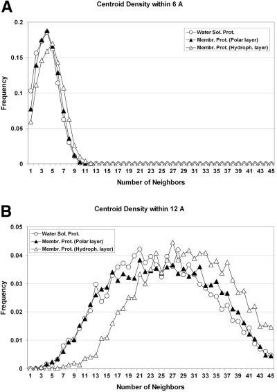
Residue density profiles observed in the hydrophobic and polar layers of the membrane and α-helical type water-soluble proteins.

Structure Generation

We designed a novel sampling strategy for predicting the structures of helical TM proteins inspired by the topologies of experimentally determined structures. We exploit the ability to predict the helical regions that span the membrane.^31-36,44,45 The focus of our search strategy is to efficiently generate structures with the predicted TM helices in positions that are consistent with spanning the membrane. Sampling from the space of possible spanning arrangements is nontrivial because of the interdependence caused by the connectivity of the peptide backbone. Because of lever arm effects, small changes in backbone torsion angles can cause large-scale motions, possibly leading to configurations that could not span the membrane. We get around this global sensitivity to local perturbations by not requiring all configurations to span the membrane all the time. Instead, we build up the structure helix by helix starting from a helix near the middle of the protein. After 18,000 attempted Monte Carlo moves, a new helix is added at either the N- or C-terminus (chosen randomly). This embedding procedure favors, but does not enforce, interaction of neighboring helices in sequence—a tendency that is also observed in membrane protein structures, where about 75% of sequence-adjacent helices interact with each other.⁴³ This approach simplifies finding structures that span the membrane, by incrementally solving the sub-problem of finding arrangements of subsets of helices that span membrane.

De novo Prediction of Membrane Protein Structures From Sequence

We tested the method on 12 membrane protein sequences for which the structure is known (see Table IV). Five thousand models were generated for each of the 12 proteins followed by clustering.⁴⁶ In addition to evaluating the RMSD of the cluster centers to the native structure (Fig. 4 and Table 2S in Supplementary Material), we also performed global distance test (GDT⁴⁷) calculations to identify regions of local as well as global structural similarity between the models and the native structure. Figure 5 shows that the cluster centers span a broad range of RMSDs to the native structure, both over the whole structure and over subsets of the structure. This wide range suggests the better predictions are considerably closer to the correct structure than would be expected by chance: Inspection of similar plots for CASP predictions (http://www2.predictioncenter.org/casp/casp6/public/cgibin/results.cgi) shows that for very difficult targets, where no good predictions were made, the lines for different models are relatively closely bundled. This is also observed for our poor predictions of 7-Helix Subdomain of H⁺/Cl⁻ Exchange Transporter [Fig. 5(K)].

TABLE IV.

Membrane Proteins Tested Using Rosetta-Membrane Method

No.	Protein name	PDB code	Resolution (Å)	Number of TM helices	Total number of residues	Residue numbers in chain
1	Bacteriorhodopsin (full length)	1PY6	1.8	7	227	5–231
2	Subdomain of bacteriorhodopsin	1PY6	1.8	4	123	77–199
3	Subdomain of cytochrome C oxidase aa3	1OCC	2.8	5	191	71–261 (chain C)
4	Subdomain of lactose permease transporter	1PV6	3.5	6	190	1–190
5	Subdomain of aquaporin water channel AQP1	1J4N	2.2	3	116	4–119
6	Subdomain of fumarate reductase complex	1QLA	2.2	5	217	21–237 (chain C)
7	Subdomain of V-type Na+-ATPase	2BL2	2.1	4	145	12–156
8	Subdomain of nicotinic acetylcholine receptor	2BG9	4.0	3	91	211–301 (chain A)
9	Subdomain of multidrug efflux transporter	1IWG	3.5	5	168	330–497
10	Subdomain of SecYEβ protein-conducting channel	1RHZ	3.5	5	166	23–188 (chain A)
11	Subdomain of H+/Cl− exchange transporter	1KPL	3.0	7	203	31–233
12	Rhodopsin	1U19	2.2	7	278	33–310

Fig. 4.

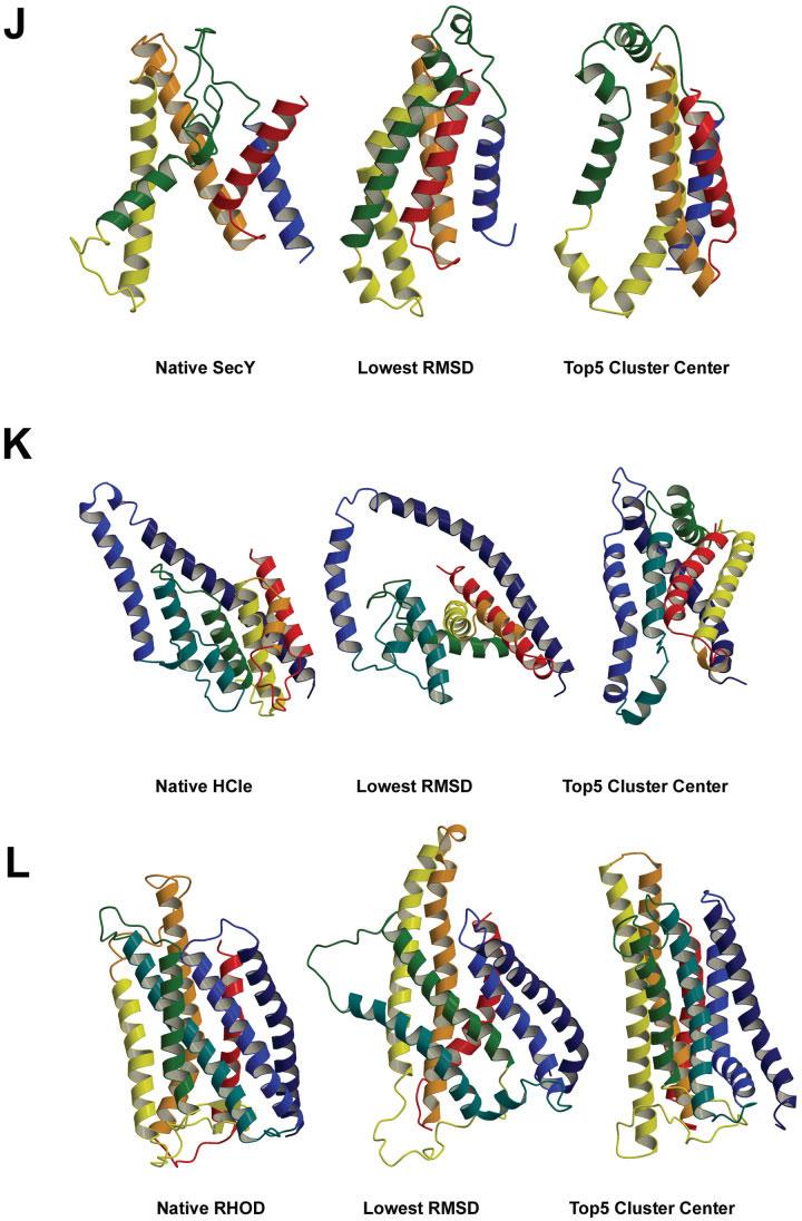
The best RMSD model and one of top five cluster center models compared with the native structure for each tested membrane protein. A: 7 TM helix bacteriorhodopsin (BRD7). B: 4 TM helix bacteriorhodopsin (BRD4). C: 5 TM helix subdomain of cytochrome C oxidase (CytC). D: 6 TM helix subdomain of lactose permease transporter (LtpA). E: 3 TM helix subdomain of aquaporin water channel (Aqp1). F: 5 TM helix subdomain of fumarate reductase complex (FmrC). G: 4 TM helix subdomain of V-type Na⁺-ATPase (VATP). H: 3 TM helix subdomain of nicotinic acetylcholine receptor (NACR). I: 5 TM helix subdomain of multidrug efflux transporter (AcrB). J: 5 TM helix subdomain of SecYEβ protein-conducting channel (SecY). K: 7 TM helix subdomain of H⁺/Cl⁻ exchange transporter (HCle). L: 7 TM helix rhodopsin (RHOD).

Fig. 5.

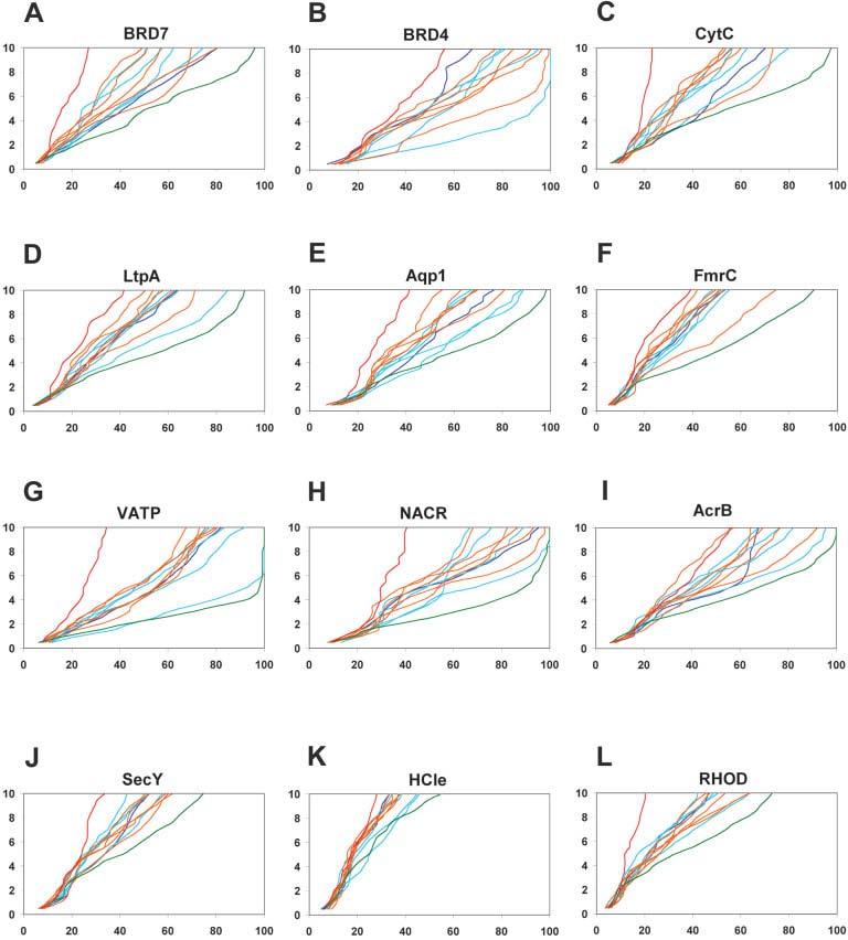
Global distance test (GDT⁴⁷) plots for all membrane proteins tested. The y axis represents a C_α distance cutoff (in Angstroms) under which the model was fitted to the native structure, and the x axis represents the percentage of C_α atoms in the model that fit below that distance cutoff value. Dark blue—the largest cluster center, cyan—cluster centers 2–5, orange—cluster centers 6–10, green—best RMSD model, and red—worst RMSD model. A: 7 TM helix bacteriorhodopsin (BRD7). B: 4 TM helix bacteriorhodopsin (BRD4). Cluster center model 2 for BRD4 is also the best RMSD model and shown in cyan. C: 5 TM helix subdomain of cytochrome C oxidase (CytC). D: 6 TM helix subdomain of lactose permease transporter (LtpA). E: 3 TM helix subdomain of aquaporin water channel (Aqp1). F: 5 TM helix subdomain of fumarate reductase complex (FmrC). G: 4 TM helix subdomain of V-type Na⁺-ATPase (VATP). H: 3 TM helix subdomain of nicotinic acetylcholine receptor (NACR). I: 5 TM helix subdomain of multidrug efflux transporter (AcrB). J: 5 TM helix subdomain of SecYEβ protein-conducting channel (SecY). K: 7 TM helix subdomain of H^_/Cl⁻ exchange transporter (HCle). L: 7 TM helix rhodopsin (RHOD).

Results for each of the 12 protein targets are described in the following section.

Bacteriorhodopsin (7 helices)

Bacteriorhodopsin (PDB code 1PY6) is a representative of a family of bacterial rhodopsin structures—currently the largest family of membrane protein structures⁵ available in the PDB.⁶ The structure of bacterial rhodopsins has a relatively simple topology where each consecutive TM segment interacts with the previous TM segment in the sequence with an overall counterclockwise order if viewed from the extracellular side of the membrane.⁴⁸ The extracellular loop between the TM helices 2 and 3 contains β-strand structure and is much longer (∼18 residues) than the other loops connecting the TM helices in the structure, which are 4–6 residues long. The top cluster center had an RMSD of 8.7 Å to the native structure over all 227 residues and an RMSD of 3.9 Å over 121 residues [Fig. 4(A)]. The lowest RMSD model in this cluster had an RMSD to native of just 6.3 Å and an RMSD of 3.6 Å over 126 residues—a quite low value for de novo prediction of a protein sequence with 227 residues [Fig. 4(A)]. The β-strand in the loop between TM helices 2 and 3 was not predicted because the strands were poorly predicted by the secondary structure prediction method^49,50 used to generate structure fragments (data not shown). The packing residue density was not significantly different between Rosetta-Membrane models and the native structures for all membrane proteins tested (data not shown), although some of the models appear more compact in the figures. Modeling of prosthetic groups attached to bacteriorhodopsin is not possible during the low-resolution protein structure prediction reported in this article; however, it will be possible during future full atom structure refinement calculations (see Discussion below).

4-Helix subdomain of bacteriorhodopsin

To test whether our method is able to predict with higher resolution portions of membrane proteins closer to the length range where soluble proteins structure prediction has been successful, we also attempted to predict just the middle four helices (TM helices 3–6) of bacteriorhodopsin (PDB code 1PY6). One of the five largest cluster centers had 3.1 Å RMSD over all 123 residues and this model had the lowest RMSD value in the set [Fig. 4(B)].

5-Helix subdomain of cytochrome C oxidase

To test whether our method can also predict membrane protein structures with more complicated topology, we first attempted to predict a five TM helix subdomain of chain C of the cytochrome C oxidase (PDB code 1OCC). This protein in addition to four closely packed helices (similarly to the four helices subdomain of the bacteriorhodopsin) has an N-terminal TM helix (helix 1) interacting with the C-terminal two helices (helices 4 and 5) but not with the nearby two helices in the sequence (helices 2 and 3) [Fig. 4(C)]. In addition, there is a long (∼23 residues) loop connecting the TM helices 1 and 2. Our best model among the top five cluster centers was predicted with 8.3 Å RMSD over all 191 residues and an RMSD of 3.7 Å over 102 residues. The lowest RMSD model had an RMSD of 6.0 Å to the native and an RMSD of 3.9 Å over 123 residues [Fig. 4(C)].

6-Helix subdomain of lactose permease transporter

We also attempted to predict the more complicated topology of the TM helices observed in a six TM helix subdomain of lactose permease transporter (PDB code 1PV6). In contrast to the relatively simple arrangement of the TM helices in the structure of the bacteriorhodopsin [Fig. 4(A)], in lactose permease transporter each of the TM helices has little or no contact with the next or previous TM segment in the sequence [Fig. 4(D)]. Our best model among the top five cluster centers had an RMSD of 8.9 Å to the native structure over all 190 residues and an RMSD of 3.9 Å over 104 residues [Fig. 4(D)]. The lowest RMSD model was in this cluster and had an RMSD to the native of 6.5 Å over all 190 residues and an RMSD of 4.0 Å over 134 residues [Fig. 4(D)].

3-Helix subdomain of aquaporin water channel

To test the performance of our method on membrane proteins with relatively short α-helical segments in the loops between the TM helices, we first attempted to model 3 TM helices subdomain of the aquaporin water channel structure, which represents about half of aquaporin's quasi-twofold symmetric structure. TM helices 2 and 3 do not interact with each other in the structure and are connected by ∼18-residues-long loop that contains a 10-residue α-helix. Our best model among the top five cluster centers had an RMSD to the native of 6.8 Å over all 116 residues and an RMSD of 3.8 Å over 86 residues [Fig. 4(E)]. The lowest RMSD model in this cluster had an RMSD value of 5.4 Å to the native over all 116 residues and an RMSD of 3.8 Å over 86 residues [Fig. 4(E)].

5-Helix subdomain of fumarate reductase complex

We also attempted to model a five TM helix subdomain of the chain C of the fumarate reductase complex structure, which also has α-helical segments in three of four loops between the TM segments. Our method failed to predict this protein with RMSD <10 Å from the native structure as one of the top five cluster centers. The best predicted model among the top 10 cluster centers had an RMSD to the native of 8.9 Å over all 217 residues and an RMSD of 3.9 Å over 98 residues [Fig. 4(F)]. The lowest RMSD model had an RMSD to the native of 7.1 Å over all 217 residues and an RMSD of 3.9 Å over 130 residues [Fig. 4(F)].

4-Helix subdomain of V-type Na⁺-ATPase

We attempted to model a four TM helix subdomain of V-type Na⁺-ATPase (PDB code 2BL2), which has a relatively simple topology in which each of the TM helices interacts with the next or previous TM segment in the sequence [Fig. 4(G)]. This TM helix topology, however, is different from the one observed in the 4-helix subdomain of the bacteriorhodopsin [Fig. 4(B)]. Our best model among the top five cluster centers had an RMSD of 3.3 Å to the native structure over all 145 residues [Fig. 4(G)]. The lowest RMSD model was in this cluster and had an RMSD to the native of 2.9 Å over all 145 [Fig. 4(G)].

3-Helix subdomain of nicotinic acetylcholine receptor

We also modeled the three TM helix subdomain of the nicotinic acetylcholine receptor (PDB code 2BG9). This structure also has a relatively simple arrangement of the TM helices where each of the TM helices interacts with the next or previous TM segment in the sequence [Fig. 4(H)]. Our best model among the top five cluster centers had an RMSD of 3.9 Å to the native structure over all 91 residues [Fig. 4(H)]. The lowest RMSD model was in this cluster and had an RMSD to the native of 3.7 Å over all 145 [Fig. 4(H)].

5-Helix subdomain of multidrug efflux transporter

In contrast to the relatively simple arrangement of the TM helices observed in the structures of the bacteriorhodopsin [Fig. 4(A)], V-type Na⁺-ATPase [Fig. 4(G)], and nicotinic acetylcholine receptor [Fig. 4(H)], a five TM helix subdomain of the multidrug efflux transporter (PDB code 1IWG) contains TM helices that have little contact with the next or previous TM segment in the sequence [Fig. 4(I)]. Our best model among the top five cluster centers had an RMSD of 6.2 Å to the native structure over all 168 residues and an RMSD of 3.9 Å over 98 residues [Fig. 4(I)]. The lowest RMSD model was in this cluster and had an RMSD to the native of 5.0 Å over all 168 residues and an RMSD of 3.9 Å over 138 residues [Fig. 4(I)].

5-Helix subdomain of SecYEβ protein-conducting channel

To test the Rosetta-Membrane method performance on another type of channel-forming protein with a short α-helix that dips into the membrane besides aquaporin [Fig. 4(E)], we modeled a five TM helix subdomain of the SecYEβ protein-conducting channel (PDB code 1RHZ). The Rosetta-Membrane method does poorly on this relatively complex structure—our best model among the top five cluster centers had an RMSD of 12.8 Å to the native structure over all 166 residues and an RMSD of 3.5 Å over just 51 residues [Fig. 4(J)]. The lowest RMSD model had an RMSD to the native of 8.7 Å over all 166 residues and an RMSD of 3.9 Å over 77 residues [Fig. 4(J)]. GDT analysis shows that our best predictions are better than random models [Fig. 5(J)].

7-Helix subdomain of H⁺/Cl⁻ exchange transporter

To test the Rosetta-Membrane method performance on a membrane protein with even more complex topology, we attempted to model a seven TM helix subdomain of the H⁺/Cl⁻ exchange transporter (formerly known as ClC chloride channel) (PDB code 1KPL). There are several features of this protein that contribute to the complexity of its structure: 1. a very long (>40 residues) first TM helix; 2. the first and second TM helices have little contact with each other; 3. five of seven TM helices are <20 residues long—very unusual for membrane proteins; 4. the second and third TM helices connected by a 25-residue-long loop with short α-helix dipping into the membrane [Fig. 4(K)]. In addition, the TM region prediction programs,^31-36,45 used to define TM regions by Rosetta-Membrane method, predicted reliably only 5 of 7 TM helices (TM helices 4 and 6 were not predicted). Rosetta-Membrane method does poorly on this complex membrane protein—our best model among the top five cluster centers had an RMSD of 16.4 Å to the native structure over all 203 residues and an RMSD of 3.6 Å over just 60 residues [Fig. 4(K)]. The lowest RMSD model had an RMSD to the native of 12.4 Å over all 202 residues and an RMSD of 3.9 Å over 58 residues [Fig. 4(K)]. GDT analysis shows that our predictions for this very complex membrane protein are the worst among the set of membrane proteins tested [Fig. 5(K)].

7-Helix rhodopsin

To test the Rosetta-Membrane method performance on a relatively long membrane protein with relatively simple TM helix topology, we attempted to model rhodopsin (PDB code 1U19). The length of the TM part with connecting loops is 278 residues for this protein—too long for the current version of the Rosetta-Membrane method to predict accurately. In addition, three of six connecting loops in rhodopsin structure are >10 residues long, whereas there is only one such loop in the bacteriorhodopsin structure [Fig. 4(A)]. Our best model among the top five cluster centers had an RMSD of 10.2 Å to the native structure over all 278 residues and an RMSD of 3.6 Å over just 55 residues [Fig. 4(L)]. The lowest RMSD model had an RMSD to the native of 9.2 Å over all 278 residues and an RMSD of 3.8 Å over 91 residues [Fig. 4(L)]. Despite the relatively large size of this protein, our best predictions are considerably better than random models [Fig. 5(L)].

DISCUSSION

Our method may mimic aspects of the folding of membrane proteins in cells. It appears that TM helices emerge from the translocon as they are being translated on the ribosome soon after translocation into the membrane.⁵¹ These preformed helices then assemble together in the membrane.⁵² This is also similar to the two-stage model of Popot and Engelman.⁵³ By building up the structure through the sequential addition of helices, we may be following the same pathways that the physical protein uses to reach its native state.

We do find that some orders of assembly are more productive than others in the context of our algorithm. For example the central 4 (C, D, E, F) helices of bacteriorhodopsin form a substructure that our method can accurately fold in the absence of the N- and C-terminal helices (A, B, G). This is consistent with the data that show that subsets of helices of bacteriorhodopsin can be independently stable.⁵⁴ Our results suggest that the most productive pathway of assembly may not be the strictly N-terminus to C-terminus of translation.

Comparison to Other De Novo Prediction Methods

Over the past decade, a number of different methods have been developed to predict helical TM proteins de novo.^55-63 Taylor et al.⁵⁵ achieved RMSD of 6.0 Å to the helical regions in the bacteriorhodopsin using MSA information and some structural constraints. Using structural constraints and/or ideal α-helices, RMSD values <1 Å from the glycophorin A NMR structure have been obtained using several methods.^56-58,61,64 Shacham et al.^62,63 also used structural constraints and experimental data to model bacteriorhodopsin and obtained RMSD value of 3.9 Å to the native structure. Kim et al.⁵⁹ developed a method that uses the oligomerization state of a protein as the only structural constraint during simulations and predicted the glycophorin A structure with an RMSD of 1.9 Å. PellegriniCalace et al.⁶⁰ adopted their knowledge-based FRAG-FOLD^65,66 method to model helical TM proteins by addition of membrane-specific energy terms derived from the known helical TM proteins structures using membrane layer representation similar to ours, and their de novo simulations of one- and two-helix proteins generated best models with RMSD values ranging from 3.6 to 6.5 Å. Other research groups have developed methods to predict TM protein structures using low-resolution cryo-electron microscopy data and residue conservation profiles.^67-70 For example, using these data, Baldwin et al.,⁶⁷ Fleishman et al.,⁶⁹ and Beuming and Weinstein⁷⁰ constructed models of rhodopsin with RMSDs of 3.2, 3.7, and 3.0 Å to the native structure,^71,72 respectively. In contrast to these earlier structure predictions of small helix TM proteins, we predicted multipass helical TM proteins without using structural constraints or experimental data and our results compare favorably with the previous results. For three- and four-helix TM proteins, we predicted between 67 and 145 residues <4 Å RMSD from the native structure and for five-, six-, and seven-helix TM proteins, we predicted between 51 and 121 residues <4 Å RMSD from the native structure (see Table 2S in Supplementary Material). These values are comparable to the accuracy of low-resolution predictions made by the Rosetta method for water-soluble proteins of the same length.⁷ The FRAGFOLD method has been recently extended to multipass helical bundles and also has had encouraging results (David Jones, personal communication).

These results indicate that the Rosetta-Membrane method is capable of generating models with accuracy in the range of de novo methods, such as Rosetta, developed for prediction of water-soluble proteins. Because the membrane bilayer provides strong constraints, de novo prediction of membrane protein structures may be easier than water-soluble protein structures of the same sequence length. However, multipass membrane proteins are generally much longer than the single-domain globular proteins on which de novo methods had some success. Unfortunately, because of the formidable sampling problem, our results for large and complex proteins are in general poor whether they be integral membrane or soluble.

Directions for Future Work

The results reported herein present our first attempt to model helical TM proteins using the Rosetta-Membrane method. Although encouraging progress has been made, further improvements of the method are clearly necessary to generate higher-resolution helical TM protein structures. In the present low-resolution version of the method, residue side-chains are represented just by a single centroid atom and specific side-chain packing is not modeled, and our next step will be development of the Rosetta-Membrane high-resolution full-atom method that will account for van der Waals, hydrogen bonds, and lipid and solvent interactions. Use of residue conservation information from the homologous sequences should improve prediction of residue exposure to the lipid environment.⁵⁶ Incorporation of symmetry should improve accuracy considerably for oligomeric proteins.⁵⁹ Prediction of structures for many homologous protein sequences along with the sequence of interest has led to significant improvement in accuracy in small water-soluble protein structure prediction^8,9 and we will test a similar approach for helical TM proteins. More accurate modeling of TM proteins with complex helix topology may be possible with a recently developed protocol that allows direct sampling of nonlocal interactions during structure assembly.⁸ Ultimately, given the large size and complexity of membrane proteins, the most important use of the methodology developed in the article may be in conjunction with experimental data from crosslinking, cryo-electron microscopy, or other methods, which provide low-resolution structural information for narrowing the conformational search.

REFERENCES

- 1.Hopkins AL, Groom CR. The druggable genome. Nat Rev Drug Discov. 2002;1(9):727–730. doi: 10.1038/nrd892. [DOI] [PubMed] [Google Scholar]
- 2.Wallin E, von Heijne G. Genome-wide analysis of integral membrane proteins from eubacterial, archaean, and eukaryotic organisms. Protein Sci. 1998;7(4):1029–1038. doi: 10.1002/pro.5560070420. [DOI] [PMC free article] [PubMed] [Google Scholar]
- 3.Arkin IT, Brunger AT, Engelman DM. Are there dominant membrane protein families with a given number of helices? Proteins. 1997;28(4):465–466. doi: 10.1002/(sici)1097-0134(199708)28:4<465::aid-prot1>3.0.co;2-9. [DOI] [PubMed] [Google Scholar]
- 4.Liu J, Rost B. Comparing function and structure between entire proteomes. Protein Sci. 2001;10(10):1970–1979. doi: 10.1110/ps.10101. [DOI] [PMC free article] [PubMed] [Google Scholar]
- 5.White SH. http://blanco.biomol.uci.edu/Membrane_Proteins_xtal.html
- 6.Berman HM, Westbrook J, Feng Z, et al. The protein data bank. Nucleic Acids Res. 2000;28(1):235–242. doi: 10.1093/nar/28.1.235. [DOI] [PMC free article] [PubMed] [Google Scholar]
- 7.Bradley P, Chivian D, Meiler J, et al. Rosetta predictions in CASP5: successes, failures, and prospects for complete automation. Proteins. 2003;53(Suppl 6):457–468. doi: 10.1002/prot.10552. [DOI] [PubMed] [Google Scholar]
- 8.Bradley P, Malmstrom L, Qian B, et al. Free modeling with Rosetta in CASP6. Proteins. doi: 10.1002/prot.20729. in press. [DOI] [PubMed] [Google Scholar]
- 9.Bradley P, Misura KM, Baker D. Toward high-resolution de novo structure prediction for small proteins. Science. 2005;309(5742):1868–1871. doi: 10.1126/science.1113801. [DOI] [PubMed] [Google Scholar]
- 10.Rees DC, DeAntonio L, Eisenberg D. Hydrophobic organization of membrane proteins. Science. 1989;245(4917):510–513. doi: 10.1126/science.2667138. [DOI] [PubMed] [Google Scholar]
- 11.Ulmschneider MB, Sansom MS, Di Nola A. Properties of integral membrane protein structures: derivation of an implicit membrane potential. Proteins. 2005;59(2):252–265. doi: 10.1002/prot.20334. [DOI] [PubMed] [Google Scholar]
- 12.Pilpel Y, Ben-Tal N, Lancet D. kPROT: a knowledge-based scale for the propensity of residue orientation in transmembrane segments. Application to membrane protein structure prediction. J Mol Biol. 1999;294(4):921–935. doi: 10.1006/jmbi.1999.3257. [DOI] [PubMed] [Google Scholar]
- 13.Adamian L, Nanda V, Degrado WF, Liang J. Empirical lipid propensities of amino acid residues in multispan alpha helical membrane proteins. Proteins. 2005;59(3):496–509. doi: 10.1002/prot.20456. [DOI] [PubMed] [Google Scholar]
- 14.Eilers M, Patel AB, Liu W, Smith SO. Comparison of helix interactions in membrane and soluble alpha-bundle proteins. Biophys J. 2002;82(5):2720–2736. doi: 10.1016/S0006-3495(02)75613-0. [DOI] [PMC free article] [PubMed] [Google Scholar]
- 15.Javadpour MM, Eilers M, Groesbeek M, Smith SO. Helix packing in polytopic membrane proteins: role of glycine in transmembrane helix association. Biophys J. 1999;77(3):1609–1618. doi: 10.1016/S0006-3495(99)77009-8. [DOI] [PMC free article] [PubMed] [Google Scholar]
- 16.Jiang S, Vakser IA. Side chains in transmembrane helices are shorter at helix–helix interfaces. Proteins. 2000;40(3):429–435. doi: 10.1002/1097-0134(20000815)40:3<429::aid-prot80>3.0.co;2-2. [DOI] [PubMed] [Google Scholar]
- 17.Jiang S, Vakser IA. Shorter side chains optimize helix–helix packing. Protein Sci. 2004;13(5):1426–1429. doi: 10.1110/ps.03505804. [DOI] [PMC free article] [PubMed] [Google Scholar]
- 18.Adamian L, Liang J. Helix–helix packing and interfacial pairwise interactions of residues in membrane proteins. J Mol Biol. 2001;311(4):891–907. doi: 10.1006/jmbi.2001.4908. [DOI] [PubMed] [Google Scholar]
- 19.Adamian L, Liang J. Interhelical hydrogen bonds and spatial motifs in membrane proteins: polar clamps and serine zippers. Proteins. 2002;47(2):209–218. doi: 10.1002/prot.10071. [DOI] [PubMed] [Google Scholar]
- 20.Choma C, Gratkowski H, Lear JD, DeGrado WF. Asparagine-mediated self-association of a model transmembrane helix. Nat Struct Biol. 2000;7(2):161–166. doi: 10.1038/72440. [DOI] [PubMed] [Google Scholar]
- 21.Gratkowski H, Lear JD, DeGrado WF. Polar side chains drive the association of model transmembrane peptides. Proc Natl Acad Sci USA. 2001;98(3):880–885. doi: 10.1073/pnas.98.3.880. [DOI] [PMC free article] [PubMed] [Google Scholar]
- 22.Zhou FX, Cocco MJ, Russ WP, Brunger AT, Engelman DM. Interhelical hydrogen bonding drives strong interactions in membrane proteins. Nat Struct Biol. 2000;7(2):154–160. doi: 10.1038/72430. [DOI] [PubMed] [Google Scholar]
- 23.Zhou FX, Merianos HJ, Brunger AT, Engelman DM. Polar residues drive association of polyleucine transmembrane helices. Proc Natl Acad Sci USA. 2001;98(5):2250–2255. doi: 10.1073/pnas.041593698. [DOI] [PMC free article] [PubMed] [Google Scholar]
- 24.Rohl CA, Strauss CE, Misura KM, Baker D. Protein structure prediction using Rosetta. Methods Enzymol. 2004;383:66–93. doi: 10.1016/S0076-6879(04)83004-0. [DOI] [PubMed] [Google Scholar]
- 25.Simons KT, Kooperberg C, Huang E, Baker D. Assembly of protein tertiary structures from fragments with similar local sequences using simulated annealing and Bayesian scoring functions. J Mol Biol. 1997;268(1):209–225. doi: 10.1006/jmbi.1997.0959. [DOI] [PubMed] [Google Scholar]
- 26.Simons KT, Ruczinski I, Kooperberg C, Fox BA, Bystroff C, Baker D. Improved recognition of native-like protein structures using a combination of sequence-dependent and sequence-independent features of proteins. Proteins. 1999;34(1):82–95. doi: 10.1002/(sici)1097-0134(19990101)34:1<82::aid-prot7>3.0.co;2-a. [DOI] [PubMed] [Google Scholar]
- 27.White SH, Wimley WC. Membrane protein folding and stability: physical principles. Annu Rev Biophys Biomol Struct. 1999;28:319–365. doi: 10.1146/annurev.biophys.28.1.319. [DOI] [PubMed] [Google Scholar]
- 28.Karplus K, Karchin R, Barrett C, et al. What is the value added by human intervention in protein structure prediction? Proteins. 2001;(Suppl 5):86–91. doi: 10.1002/prot.10021. [DOI] [PubMed] [Google Scholar]
- 29.Jones DT. Protein secondary structure prediction based on position-specific scoring matrices. J Mol Biol. 1999;292(2):195–202. doi: 10.1006/jmbi.1999.3091. [DOI] [PubMed] [Google Scholar]
- 30.Meiler J. http://www.jens-meiler.de/ JUFO3D: Secondary structure prediction for proteins from low resolution tertiary structure. 2003
- 31.Krogh A, Larsson B, von Heijne G, Sonnhammer EL. Predicting transmembrane protein topology with a hidden Markov model: application to complete genomes. J Mol Biol. 2001;305(3):567–580. doi: 10.1006/jmbi.2000.4315. [DOI] [PubMed] [Google Scholar]
- 32.Sonnhammer EL, von Heijne G, Krogh A. A hidden Markov model for predicting transmembrane helices in protein sequences. Proc Int Conf Intell Syst Mol Biol. 1998;6:175–182. [PubMed] [Google Scholar]
- 33.Hofmann K, Stoffel W. TMbase—a database of membrane spanning proteins segments. Biol Chem Hoppe Seyler. 1993;374:166. [Google Scholar]
- 34.McGuffin LJ, Bryson K, Jones DT. The PSIPRED protein structure prediction server. Bioinformatics. 2000;16(4):404–405. doi: 10.1093/bioinformatics/16.4.404. [DOI] [PubMed] [Google Scholar]
- 35.Tusnady GE, Simon I. Principles governing amino acid composition of integral membrane proteins: application to topology prediction. J Mol Biol. 1998;283(2):489–506. doi: 10.1006/jmbi.1998.2107. [DOI] [PubMed] [Google Scholar]
- 36.Tusnady GE, Simon I. The HMMTOP transmembrane topology prediction server. Bioinformatics. 2001;17(9):849–850. doi: 10.1093/bioinformatics/17.9.849. [DOI] [PubMed] [Google Scholar]
- 37.Tusnady GE, Dosztanyi Z, Simon I. Transmembrane proteins in the Protein Data Bank: identification and classification. Bioinformatics. 2004;20(17):2964–2972. doi: 10.1093/bioinformatics/bth340. [DOI] [PubMed] [Google Scholar]
- 38.Ulmschneider MB, Sansom MS. Amino acid distributions in integral membrane protein structures. Biochim Biophys Acta. 2001;1512(1):1–14. doi: 10.1016/s0005-2736(01)00299-1. [DOI] [PubMed] [Google Scholar]
- 39.Yau WM, Wimley WC, Gawrisch K, White SH. The preference of tryptophan for membrane interfaces. Biochemistry. 1998;37(42):14713–14718. doi: 10.1021/bi980809c. [DOI] [PubMed] [Google Scholar]
- 40.Schiffer M, Chang CH, Stevens FJ. The functions of tryptophan residues in membrane proteins. Protein Eng. 1992;5(3):213–214. doi: 10.1093/protein/5.3.213. [DOI] [PubMed] [Google Scholar]
- 41.Eilers M, Shekar SC, Shieh T, Smith SO, Fleming PJ. Internal packing of helical membrane proteins. Proc Natl Acad Sci USA. 2000;97(11):5796–5801. doi: 10.1073/pnas.97.11.5796. [DOI] [PMC free article] [PubMed] [Google Scholar]
- 42.Liu W, Eilers M, Patel AB, Smith SO. Helix packing moments reveal diversity and conservation in membrane protein structure. J Mol Biol. 2004;337(3):713–729. doi: 10.1016/j.jmb.2004.02.001. [DOI] [PubMed] [Google Scholar]
- 43.Gimpelev M, Forrest LR, Murray D, Honig B. Helical packing patterns in membrane and soluble proteins. Biophys J. 2004;87(6):4075–4086. doi: 10.1529/biophysj.104.049288. [DOI] [PMC free article] [PubMed] [Google Scholar]
- 44.Jones DT. Do transmembrane protein superfolds exist? FEBS Lett. 1998;423(3):281–285. doi: 10.1016/s0014-5793(98)00095-7. [DOI] [PubMed] [Google Scholar]
- 45.Jones DT, Taylor WR, Thornton JM. A model recognition approach to the prediction of all-helical membrane protein structure and topology. Biochemistry. 1994;33(10):3038–3049. doi: 10.1021/bi00176a037. [DOI] [PubMed] [Google Scholar]
- 46.Bonneau R, Strauss CE, Rohl CA, et al. De novo prediction of three-dimensional structures for major protein families. J Mol Biol. 2002;322(1):65–78. doi: 10.1016/s0022-2836(02)00698-8. [DOI] [PubMed] [Google Scholar]
- 47.Zemla A. LGA: a method for finding 3D similarities in protein structures. Nucleic Acids Res. 2003;31(13):3370–3374. doi: 10.1093/nar/gkg571. [DOI] [PMC free article] [PubMed] [Google Scholar]
- 48.Pebay-Peyroula E, Rummel G, Rosenbusch JP, Landau EM. X-ray structure of bacteriorhodopsin at 2.5 angstroms from microcrystals grown in lipidic cubic phases. Science. 1997;277(5332):1676–1681. doi: 10.1126/science.277.5332.1676. [DOI] [PubMed] [Google Scholar]
- 49.Karplus K, Barrett C, Hughey R. Hidden Markov models for detecting remote protein homologies. Bioinformatics. 1998;14(10):846–856. doi: 10.1093/bioinformatics/14.10.846. [DOI] [PubMed] [Google Scholar]
- 50.Park J, Karplus K, Barrett C, et al. Sequence comparisons using multiple sequences detect three times as many remote homologues as pairwise methods. J Mol Biol. 1998;284(4):1201–1210. doi: 10.1006/jmbi.1998.2221. [DOI] [PubMed] [Google Scholar]
- 51.Van den Berg B, Clemons WM, Jr, Collinson I, et al. X-ray structure of a protein-conducting channel. Nature. 2004;427(6969):36–44. doi: 10.1038/nature02218. [DOI] [PubMed] [Google Scholar]
- 52.Higy M, Junne T, Spiess M. Topogenesis of membrane proteins at the endoplasmic reticulum. Biochemistry. 2004;43(40):12716–12722. doi: 10.1021/bi048368m. [DOI] [PubMed] [Google Scholar]
- 53.Popot JL, Engelman DM. Helical membrane protein folding, stability, and evolution. Annu Rev Biochem. 2000;69:881–922. doi: 10.1146/annurev.biochem.69.1.881. [DOI] [PubMed] [Google Scholar]
- 54.Marti T. Refolding of bacteriorhodopsin from expressed polypeptide fragments. J Biol Chem. 1998;273(15):9312–9322. doi: 10.1074/jbc.273.15.9312. [DOI] [PubMed] [Google Scholar]
- 55.Taylor WR, Jones DT, Green NM. A method for alpha-helical integral membrane protein fold prediction. Proteins. 1994;18(3):281–294. doi: 10.1002/prot.340180309. [DOI] [PubMed] [Google Scholar]
- 56.Briggs JA, Torres J, Arkin IT. A new method to model membrane protein structure based on silent amino acid substitutions. Proteins. 2001;44(3):370–375. doi: 10.1002/prot.1102. [DOI] [PubMed] [Google Scholar]
- 57.Dobbs H, Orlandini E, Bonaccini R, Seno F. Optimal potentials for predicting inter-helical packing in transmembrane proteins. Proteins. 2002;49(3):342–349. doi: 10.1002/prot.10229. [DOI] [PubMed] [Google Scholar]
- 58.Fleishman SJ, Ben-Tal N. A novel scoring function for predicting the conformations of tightly packed pairs of transmembrane alpha-helices. J Mol Biol. 2002;321(2):363–378. doi: 10.1016/s0022-2836(02)00590-9. [DOI] [PubMed] [Google Scholar]
- 59.Kim S, Chamberlain AK, Bowie JU. A simple method for modeling transmembrane helix oligomers. J Mol Biol. 2003;329(4):831–840. doi: 10.1016/s0022-2836(03)00521-7. [DOI] [PubMed] [Google Scholar]
- 60.Pellegrini-Calace M, Carotti A, Jones DT. Folding in lipid membranes (FILM): a novel method for the prediction of small membrane protein 3D structures. Proteins. 2003;50(4):537–545. doi: 10.1002/prot.10304. [DOI] [PubMed] [Google Scholar]
- 61.Pappu RV, Marshall GR, Ponder JW. A potential smoothing algorithm accurately predicts transmembrane helix packing. Nat Struct Biol. 1999;6(1):50–55. doi: 10.1038/4922. [DOI] [PubMed] [Google Scholar]
- 62.Shacham S, Marantz Y, Bar-Haim S, et al. PREDICT modeling and in-silico screening for G-protein coupled receptors. Proteins. 2004;57(1):51–86. doi: 10.1002/prot.20195. [DOI] [PubMed] [Google Scholar]
- 63.Shacham S, Topf M, Avisar N, et al. Modeling the 3D structure of GPCRs from sequence. Med Res Rev. 2001;21(5):472–483. doi: 10.1002/med.1019. [DOI] [PubMed] [Google Scholar]
- 64.Park Y, Elsner M, Staritzbichler R, Helms V. Novel scoring function for modeling structures of oligomers of transmembrane alpha-helices. Proteins. 2004;57(3):577–585. doi: 10.1002/prot.20229. [DOI] [PubMed] [Google Scholar]
- 65.Jones DT. Successful ab initio prediction of the tertiary structure of NK-lysin using multiple sequences and recognized supersecondary structural motifs. Proteins. 1997;(Suppl 1):185–191. doi: 10.1002/(sici)1097-0134(1997)1+<185::aid-prot24>3.3.co;2-t. [DOI] [PubMed] [Google Scholar]
- 66.Jones DT. Predicting novel protein folds by using FRAGFOLD. Proteins. 2001;(Suppl 5):127–132. doi: 10.1002/prot.1171. [DOI] [PubMed] [Google Scholar]
- 67.Baldwin JM, Schertler GF, Unger VM. An alpha-carbon template for the transmembrane helices in the rhodopsin family of G-protein-coupled receptors. J Mol Biol. 1997;272(1):144–164. doi: 10.1006/jmbi.1997.1240. [DOI] [PubMed] [Google Scholar]
- 68.Sorgen PL, Hu Y, Guan L, Kaback HR, Girvin ME. An approach to membrane protein structure without crystals. Proc Natl Acad Sci USA. 2002;99(22):14037–14040. doi: 10.1073/pnas.182552199. [DOI] [PMC free article] [PubMed] [Google Scholar]
- 69.Fleishman SJ, Harrington S, Friesner RA, Honig B, Ben-Tal N. An automatic method for predicting transmembrane protein structures using cryo-EM and evolutionary data. Biophys J. 2004;87(5):3448–3459. doi: 10.1529/biophysj.104.046417. [DOI] [PMC free article] [PubMed] [Google Scholar]
- 70.Beuming T, Weinstein H. Modeling membrane proteins based on low-resolution electron microscopy maps: a template for the TM domains of the oxalate transporter OxlT. Protein Eng Des Sel. 2005;18(3):119–125. doi: 10.1093/protein/gzi013. [DOI] [PubMed] [Google Scholar]
- 71.Bourne HR, Meng EC. Structure: rhodopsin sees the light. Science. 2000;289(5480):733–734. doi: 10.1126/science.289.5480.733. [DOI] [PubMed] [Google Scholar]
- 72.Palczewski K, Kumasaka T, Hori T, et al. Crystal structure of rhodopsin: a G protein-coupled receptor. Science. 2000;289(5480):739–745. doi: 10.1126/science.289.5480.739. [DOI] [PubMed] [Google Scholar]
Associated Data
This section collects any data citations, data availability statements, or supplementary materials included in this article.