Activities and Sensitivities in Boolean Network Models

Abstract

We study how the notions of importance of variables in Boolean functions as well as the sensitivities of the functions to changes in these variables impact the dynamical behavior of Boolean networks. The activity of a variable captures its influence on the output of the function and is a measure of that variable's importance. The average sensitivity of a Boolean function captures the smoothness of the function and is related to its internal homogeneity. In a random Boolean network, we show that the expected average sensitivity determines the well-known critical transition curve. We also discuss canalizing functions and the fact that the canalizing variables enjoy higher importance, as measured by their activities, than the noncanalizing variables. Finally, we demonstrate the important role of the average sensitivity in determining the dynamical behavior of a Boolean network.

Introduction.—Boolean networks are complex systems that were initially proposed as models of genetic regulatory networks [1,2] but have since been used to model a range of complex phenomena [3]. It is well known that the bias (internal homogeneity) as well as the number of input variables (network connectivity) can modulate the order-disorder transition, with higher homogeneity and lower connectivity leading to more ordered behavior. In addition, networks constructed from functions belonging to various classes, such as canalizing functions [2] and certain Post classes [4], can also exhibit a tendency toward ordered behavior.

In the original formulation [1], the connectivity is set to a constant K. However, it is also possible to let it be random, chosen under various distributions [5,6], with mean connectivity K. Another important parameter is the bias p of the random functions f_i, which is the probability that the function takes on the value 1. A random Boolean function with bias p can be generated by flipping a p-biased coin 2^K times and thus filling in the truth table. If p = 0.5, then the function is said to be unbiased. By varying the parameters K and p, the network can be made to undergo a dynamical phase transition. For example, in the case of unbiased functions, the critical connectivity is K = 2, meaning that for K > 2, we observe chaotic behavior. In general, for a given bias p, the critical connectivity is equal to K_c = [2p(1 − p)]⁻¹ (Ref. [7]). Thus, if K < K_c, perturbations die out and if K > K_c, the damage caused by a perturbation spreads throughout the network over time. Strongly biased functions (when p is far away from 0.5) are said to have a high degree of internal homogeneity [2] and are associated with increased order in Boolean networks.

The bias of a Boolean function is, in a sense, a global parameter that can affect only the Hamming weight (number of 1s in the truth table) of the function but is unable to capture any of its local structure. For example, a Boolean function with the truth table (0101010101010101) may have just as many 1s and 0s as a random unbiased function, but it has a very specific structure that plays a role in increasing order in a Boolean network. Of course, this example is rather extreme, since the above function is a function of only one variable (K = 1), with the other variables being fictitious. Thus, out of four variables, this one variable has all the importance whereas the other three variables have no importance, as their values have no way of altering the output of the function. There is reason to suppose that if we were to allow gradations of this notion of importance, then functions in which few variables have high importance and most other variables have low importance would play a similar role in eliciting order from Boolean networks. In a sense, a network comprised of such types of functions, despite possibly having a large actual connectivity, would exhibit a low virtual connectivity, as most input variables in any given function would have very little say in what happens to the function output.

The same phenomenon manifests itself in the class of so-called canalizing functions, which are known to play a role in preventing chaotic behavior [1,2,8,9]. A canalizing function is one in which at least one of the input variables (called canalizing variables) has one value that is able to determine the value of the output of the function, regardless of the other variables. There is also evidence that many control rules governing transcription of eukaryotic genes are canalizing when viewed in the Boolean formalism [10]. Although we have not yet defined a formal notion of the importance of variables, one would expect that the canalizing variables exhibit higher importance than the noncanalizing variables.

The tools that we will use to study the relative importance of variables and the effects on the behavior of Boolean networks are based on partial derivatives of Boolean functions, activities of variables, and sensitivities of Boolean functions. We should mention in passing that much of the discussion in this Letter can be formulated in terms of spectral methods or harmonic analysis on the n cube.

Activities and sensitivities.—In a Boolean function, some variables have a greater influence over the output of the function than other variables. To formalize this concept, let f: {0, 1}^K → {0, 1} be a Boolean function of K variables x₁, … , x_K. Let

$$\partial f\left(\mathbf{x}\right)∕\partial x_j=f\left({\mathbf{x}}^{(j,0)}\right)\oplus f\left({\mathbf{x}}^{(j,1)}\right)$$

be the partial derivative of f with respect to x_j, where ⊕ is addition modulo 2 (exclusive OR) and x^{(j, k)} = (x₁, …,x_j−1, K, x_j+1,…,x_K), k = 0, 1. Clearly, the partial derivative is a Boolean function itself that specifies whether a change in the jth input causes a change in the original function f. It should be noted that the Boolean derivative was recently used to develop a new order parameter for the random Boolean network phase transition [11].

Now, the activity of variable x_j in function f can be defined as

$${\alpha }_j^f=\frac{1}{2^K}\sum _{\mathbf{x}\in {\{0,1\}}^K}\partial f\left(\mathbf{x}\right)∕\partial x_j.$$

Note that although the vector x consists of K components (variables), the jth variable is fictitious in ∂f(x)/∂x_j. A variable x_j is fictitious in f if f(x^{(j, 1)}) for all x^{(j, 0)} and x^{(j, 1)}. For a K-variable Boolean function f, we can form its activity vector ${\alpha }^f=[{\alpha }_1^f,\dots ,{\alpha }_K^f]$. It is easy to see that $0\le {\alpha }_j^f\le 1$, for any j = 1,…,K. In fact, we can consider ${\alpha }_j^f$ to be a probability that toggling the jth input bit changes the function value, when the input vectors x are distributed uniformly over {0, 1}^K. Since we are in the binary setting, the activity is also the expectation of the partial derivative with respect to the uniform distribution: ${\alpha }_j^f=E[\partial f\left(\mathbf{x}\right)∕\partial x_j]$. Under an arbitrary distribution, ${\alpha }_j^f$ is referred to as the influence of variable x_j on the function f [12]. The influence of variables was used in the context of genetic regulatory network modeling in [13].

Another important quantity is the sensitivity of a Boolean function f, which measures how sensitive the output of the function is to changes in the inputs (this was introduced in [14] under the name of critical complexity). The sensitivity s^f (x) of f on vector x is defined as the number of Hamming neighbors of x on which the function value is different than on x (two vectors are Hamming neighbors if they differ in only one component). That is,

$$\begin{array}{cc}\hfill S^f\left(\mathbf{x}\right)& =\mid \{i\in [1,\dots ,K]:f\left(\mathbf{x}\oplus e_i\right)\ne f\left(\mathbf{x}\right)\}\mid \hfill \\ \hfill & =\sum _{i=1}^K\chi [f\left(\mathbf{x}\oplus e_i\right)\ne f\left(\mathbf{x}\right)],\hfill \end{array}$$

where e_i is the unit vector with 1 in the ith position and 0s everywhere else, and χ [A] is an indicator function that is equal to one if and only if A is true. The average sensitivity s^f is defined by taking the expectation of s^f (x) with respect to the distribution of x. It is easy to see that under the uniform distribution, the average sensitivity is equal to the sum of the activities:

$$S^f=E\left[S^f\left(\mathbf{x}\right)\right]=\sum _{i=1}^{K}E[\chi [f\left(\mathbf{x}\oplus e_i\right)\ne f\left(\mathbf{x}\right)]]=\sum _{i=1}^K{\alpha }_i^f.$$

Therefore, s^f is a number between 0 and K.

Intuitively speaking, it seems that the average sensitivity of a function should be related to its internal homogeneity. If a function is highly homogeneous, meaning that it has either many 1s or many 0s, then it would be unlikely to change much between neighboring vectors on the K-dimensional hypercube and hence, its average sensitivity should be low. On the other hand, a function that is not homogeneous, with roughly equal numbers of 1s and 0s, should exhibit high average sensitivity. These ideas are correct in the probabilistic sense.

Consider a random Boolean function with bias p. The truth table of such a function is a 2^K-length vector of independent and identically distributed Bernoulli (p) random variables. Therefore, the probability that two Hamming neighbors are different is equal to 2p (1 − p), since one can be 1 (with probability p) and the other 0 (with probability 1 − p), and vice versa. Since this is the same for all Hamming neighbors, all expected activities should be equal. That is, for each $i=1,\dots ,K,E\left[{\alpha }_j^f\right]=2p(1-p)$, where the expectation is taken with respect to the distribution of the truth table of the function f. Thus, the expectation of the average sensitivity is $E\left[s^f\right]={\Sigma }_{i=1}^{K}E\left[{\alpha }_i^f\right]={\Sigma }_{i=1}^{K}2p(1-p)=K2p(1-p)$. We can conclude that highly biased functions (p far away from 0.5) are expected to have low average sensitivity. Similarly, an unbiased function (p = 0.5) has expected average sensitivity equal to K/2. It is interesting to note that in the context of random Boolean networks with connectivity K, the expected average sensitivity determines the well-known critical transition curve with the Lyapunov exponent [11] being the logarithm of the expected average sensitivity: λ = logE[s^f].

Consider Fig. 1. We have generated all functions of K = 4 variables and generated a 2-dimensional normalized histogram that shows the probability that, given a normalized Hamming weight (ranging from 0 to 1), a randomly selected function has a particular average sensitivity (ranging from 0 to 4). The thick black line shows the mean average sensitivity for each Hamming weight. It is evident that the black line follows exactly the quadratic expression given by K2p(1 − p).

FIG. 1.

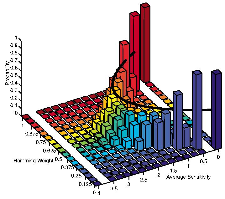
(color online). A 2-dimensional normalized histogram constructed by generating all Boolean functions of K 4 variables and computing the number of functions with a given normalized Hamming weight (which is the Hamming weight divided by 16) and with a given average sensitivity. For each fixed Hamming weight, the histogram of average sensitivities is normalized such that the sum is equal to 1, so that we can interpret each bar as a probability.

Activities of variables in canalizing functions.— A function f is said to be canalizing if there exists an i ∈ {1,…,K} and u, v ∈ {0, 1}, such that for all x₁, … , x_K ∈ {0, 1}, if x_i = u then f(x₁,…,x_K) = v. The input variable x_i is called the canalizing variable with canalizing value u and canalized value u. It is easy to show that a canalizing function f can be written either as $f(x_1,\dots ,x_K)=x_i^q\vee g(x_1,\dots ,x_{i-1},x_{i+1},\dots ,x_K)$ or $f(x_1,\dots ,x_K)=x_i^q\wedge g(x_1,\dots ,x_{i-1},x_{i+1},\dots ,x_K)$, where q ∈ {0, 1} and ⋁ and Λ denote disjunction (OR) and conjunction (AND). Here, $x_i^1=x_i$ and $x_i^0=x_i^{\prime }$, where $x_i^{\prime }$ is the complement or negation of x_i. As we already mentioned, it should be expected that in canalizing functions, the importance of canalizing variables is higher than that of noncanalizing variables. This can indeed be shown by using activities.

To illustrate this point for the particular case of only one canalizing variable, we can consider a random canalizing function of the form f(x₁, …, x_K) = x₁ ⋁ g(x₂, …, x_K), where g is chosen randomly from the set of all 2^2K−1 Boolean functions. Without loss of generality, we can suppose that the first variable, x₁, is a canalizing variable. Furthermore, the discussion for other types of canalizing functions [e.g., f(x₁, …, x_K) = x₁ Λ g(x₂, …, x_K)] would be nearly identical. In order to characterize the activities of each of the variables, it suffices to examine only the activity of x₁ and x₂, since it is clear that the activities of variables x₂, … x_K will be identical in the probabilistic sense if g(x₂, … x_K is a random unbiased function. Note that activities are themselves random variables by virtue of f being random. It is fairly straightforward to show [15] that the expected activity of the canalizing variable x₁ is equal to 1/2 whereas the expected activity of x₂ and each of the other variables is 1/4. The expected activity vector is then equal to $E\left[{\alpha }^f\right]=(\frac{1}{2},\frac{1}{4},\dots ,\frac{1}{4})$ and the expected average sensitivity is equal to $E\left[s\left(f\right)\right]=\frac{1}{2}+\frac{1}{4}(K-1)=(K+1)∕4$. The situation for two or more canalizing variables is analogous. The fact that networks comprised of canalizing functions exhibit more orderly behavior relative to random networks with the same connectivity is consistent with our intuition about lower virtual connectivity of canalizing networks in light of the above results. As random unbiased networks are expected to have average sensitivity of K/2, these results also highlight the importance of the average sensitivity as an order parameter for Boolean networks.

Dynamics of Boolean networks.—Our goal here is to show that the activities of the variables of Boolean functions, and consequently their average sensitivities, can reflect the dynamical behavior of the Boolean networks constructed from these functions. We expected that if in any given function one activity is considerably higher than all the other activities, the network should have a tendency toward ordered behavior. This should also be the case when all functions are canalizing since, as discussed in the previous section, activities of canalizing variables are expected to be larger than those of noncanalizing variables.

In order to study the dynamics of networks, we will use so-called Derrida curves [2,7]. These are constructed as follows. Let x⁽¹⁾1(t) and x⁽²⁾(t) be two randomly chosen states at some time t. The normalized Hamming distance between them is $\rho \left(t\right)=\frac{1}{N}{\Sigma }_{i=1}^N\left(x_i^{\left(i\right)}\left(t\right)\oplus x_i^{\left(2\right)}\left(t\right)\right)$. Given a random Boolean network realization, let x⁽¹⁾(t + 1) and x^{(t + 1)} be the successor states of x⁽¹⁾(t), respectively. Similarly, let ρ(t + 1) be the Hamming distance between these successor states. The Derrida curve consists of plotting ρ(t + 1) versus ρ(t) and averaging over many pairs of states and random networks. If the network is operating in the chaotic regime, then small Hamming distances tend to diverge and the Derrida curve lies above the main diagonal for small initial Hamming distances. This also implies that small gene perturbations (i.e., nearby states) tend to spread farther apart and networks are sensitive to initial conditions—a hallmark of chaotic behavior. On the other hand, networks in the ordered regime exhibit convergence for nearby states, with the Derrida curve lying below the main diagonal. The more the Derrida curve lies above the main diagonal for small values of ρ(t), the more chaotic is the network.

We performed the following computer experiment. First, we generated a random Boolean network B₁ with N = 100 elements and K = 8 inputs per function such that for each random function, seven of its variables had activity approximately 0.18 and one variable (chosen randomly) had activity 0.8. Consequently, the sample mean of the average sensitivities was approximately equal to 2. The average bias of this network was approximately equal to 0.41, which was computed by averaging over all normalized Hamming weights for the 100 functions. Briefly, each function in B₁ is generated as follows. We start off with f being a randomly generated function with bias p₁ [i.e., Bernoulli (p₁)]. Then, if x_j is the variable chosen to have the high activity, then for each x^(j,0), f(x^(j,1)) = f(x^(j,0)) with probability p₂ and f(x^(j,1)) ≠ f(x^(j,0)) with probablity 1 − p₂. Parameters p₁ and p₂ can be used to control the relative differences between the high activity and the rest of the activities.

As a next step, we generated another random Boolean network B₂ with exactly the same bias. The size of the network and connectivity were also kept the same. This was done in order to control for possible confounding effects due to bias. This random network, however, was generated purely randomly such that all expected activities were equal. Since the bias was approximately p = 0.41, the expected activities were all equal to 2p(1 − p) = 0.4838 and the average sensitivity was equal to 3.87.

Figure 2 shows the Derrida plots corresponding to the two networks, B₁ and B₂, shown as solid and dashed plots, respectively. It is apparent that the network B₁ exhibits more ordered behavior than B₂. It is important to note that the internal homogeneity, which in our case is equal for both networks, fails to explain the relatively higher order observed in B₁. It is also worth mentioning that none of the functions in B₁ turned out to be canalizing. The average sensitivity,Bas stated above, was markedly different however: 2 for B₁ and 3.87 for B₂. Thus, the average sensitivity, in this case, is a much B better indicator of the dynamical behavior than the bias.

FIG. 2.

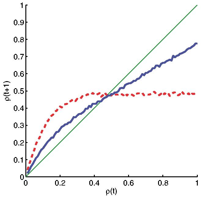
(color online). Derrida curves corresponding to two different random Boolean networks, both with N = 100 elements and K = 8 inputs in each Boolean function. The solid curve corresponds to the case where one activity is much higher than all other activities, in each Boolean function. The dashed curve corresponds to the case where all activities are equal. The internal homogeneity for both networks is the same.

Let us briefly consider another example. Consider a network with K = 18 in which every gene is governed by the function f(x₁, … ,x₁₈) = (x₁ Λ x₂) ⋁ (x₃ Λ x₄) ⋁ / ⋁ (x₁₇ Λ x₁₈). It is easy to show that each of the 18 activities is approximately equal to 0.0501 and the average sensitivity is approximately 0.0501 × 18 = 0.9010 (<1), implying the network is ordered. The normalized Hamming weight of f is 0.9249. If we construct a random Boolean network with K = 18 and bias p =0.9249, then K2p(1 − p) = 2.5001 (>1) and the network is chaotic. Thus, we can have two networks with identical connectivity and internal homogeneity that lie on opposite sides of the order-chaos boundary, with the average sensitivity reflecting this difference.

Concluding remarks.—Our results suggest that the average sensitivity is a useful order parameter in Boolean network models. In the purely random setting, the average sensitivity coincides with the well-known critical transition curve, K2p(1 − p) . However, when network functions are generated according to probability distributions that favor some variables relative to others, as measured by the activities of the variables, or when functions are chosen randomly from certain classes of functions (e.g., canalizing), we can use the average sensitivity to capture the dynamical behavior of the network. Thus, we have an analytical method that allows us to determine whether a specific network is ordered or chaotic without having to run computer simulations that construct empirical Derrida curves. For example, given a concrete network, we can compute the average sensitivity of each function and average these to obtain a single number that reflects the regime in which the network operates.

References

- 1.Kauffman SA. J. Theor. Biol. 1969;22:437. doi: 10.1016/0022-5193(69)90015-0. [DOI] [PubMed] [Google Scholar]
- 2.Kauffman SA. The Origins of Order: Self-Organization and Selection in Evolution. Oxford University Press; New York: 1993. [Google Scholar]
- 3.Aldana M, Coppersmith S, Kadanoff LP. In: Perspectives and Problems in Nonlinear Science. Kaplan E, Marsden JE, Sreenivasan KR, editors. Springer; New York: 2002. pp. 23–89. [Google Scholar]
- 4.Shmulevich I, Lähdesmäki H, Dougherty ER, Astola J, Zhang W. Proc. Natl. Acad. Sci. U.S.A. 2003;100:10 734. doi: 10.1073/pnas.1534782100. [DOI] [PMC free article] [PubMed] [Google Scholar]
- 5.Fox JJ, Hill CC. Chaos. 2001;11:809. doi: 10.1063/1.1414882. [DOI] [PubMed] [Google Scholar]
- 6.Aldana M, Cluzel P. Proc. Natl. Acad. Sci. U.S.A. 2003;100:8710. doi: 10.1073/pnas.1536783100. [DOI] [PMC free article] [PubMed] [Google Scholar]
- 7.Derrida B, Pomeau Y. Europhys. Lett. 1986;1:45. [Google Scholar]
- 8.Stauffer D. J. Stat. Phys. 1987;46:789. [Google Scholar]
- 9.Lynch JF. Random Struct. Algorithms. 1995;6:239. [Google Scholar]
- 10.Harris SE, Sawhill BK, Wuensche A, Kauffman SA. Complexity. 2002;7:23. [Google Scholar]
- 11.Luque B, Solé RV. Physica (Amsterdam) 2000;284A:33. [Google Scholar]
- 12.Kahn J, Kalai G, Linial N. Proceedings of the 29th Annual Symposium on Foundations of Computer Science. IEEE; Washington, DC: 1988. pp. 68–80. [Google Scholar]
- 13.Shmulevich I, Dougherty ER, Kim S, Zhang W. Bioinformatics. 2002;18:261. doi: 10.1093/bioinformatics/18.2.261. [DOI] [PubMed] [Google Scholar]
- 14.Cook S, Dwork C, Reischuk R. SIAM J. Comput. 1986;15:87. [Google Scholar]
- 15.See EPAPS Document No. E-PRLTAO-93-056428 for aproof that the expected activity vector of a random canalizing function with one canalizing variable is equal to 0.5, 0.25, 0:25; . . . ; 0:25. A direct link to this document may be found in the online article’s HTMLreference section. The document may also be reached via the EPAPS homepage (http://www.aip.org/pubservs/epaps.html) or from ftp.aip.org in the directory /epaps/. See the EPAPS homepage for more information.
Associated Data
This section collects any data citations, data availability statements, or supplementary materials included in this article.