An approach to electrical modeling of single and multiple cells

Abstract

Previous theoretical approaches to understanding effects of electric fields on cells have used partial differential equations such as Laplace's equation and cell models with simple shapes. Here we describe a transport lattice method illustrated by a didactic multicellular system model with irregular shapes. Each elementary membrane region includes local models for passive membrane resistance and capacitance, nonlinear active sources of the resting potential, and a hysteretic model of electroporation. Field amplification through current or voltage concentration changes with frequency, exhibiting significant spatial heterogeneity until the microwave range is reached, where cellular structure becomes almost “electrically invisible.” In the time domain, membrane electroporation exhibits significant heterogeneity but occurs mostly at invaginations and cell layers with tight junctions. Such results involve emergent behavior and emphasize the importance of using multicellular models for understanding tissue-level electric field effects in higher organisms.

Electric field effects in biological systems are of long-standing scientific interest. Endogenous fields are important in development (1) and wound healing (2). Small external fields from dc to >≈1 GHz are of interest with respect to sensory systems, medical applications, and possible human health hazards (3–12). Larger pulsed fields are involved in stimulation of excitable cells (13, 14) and electroporation and heating of tissue in vivo (15–19) and cells in vitro (20–23) or ex vivo (24).

Biological cells contain highly conductive aqueous electrolytes separated by thin, low-conductivity membranes populated with electrically active macromolecules. As a result, multicellular systems are extremely heterogeneous with respect to their passive electrical properties (local resistance and capacitance) and both passive and active interaction mechanisms (ion pumps, voltage-gated channels, and electroporatable membrane regions). This heterogeneity creates a basic complication: an applied field, E⃗_app, leads to a response field, E⃗_res, that differs spatially and temporally from E⃗_app within the biological system. Here E⃗_app is the field that would exist if the biological system were replaced by a purely conductive medium.

Many of these interactions have biological relevance. Fields guide ionic currents (1, 2) and cause Joule heating. At cell membranes fields drive conformational changes in macromolecules, particularly ion channels (7, 13, 14) and membrane-associated enzymes (6, 25), and cause electroporation (15–19, 26, 27) and the related events of electro-insertion (24) and electrofusion (22, 26, 27). Several of these interactions can take place simultaneously, although often one interaction dominates. Importantly, these interactions depend on the local electric field, not the average applied field usually reported in experimental studies or predicted by tissue-level simulations. Accordingly, it is important to create and solve increasingly realistic system models that reasonably represent real cells and multiple cells in close proximity.

To analyze a cellular response quantities such as electric potential (φ), electric field (E⃗ = −∇φ), transmembrane voltage (U_m), current density (J⃗ = E⃗/ρ; ρ = resistivity), and specific absorption rate (SAR; power dissipation per mass) (28) are sought throughout a system of one or more cells. Previous isolated cell models emphasized highly idealized and passive membranes. A recent single-cell model (29) has comprehensive conductive and dielectric properties, but represents the special case of an isolated spherical membrane without nonlinear membrane interactions. Solid tissue models avoid cellular complexity altogether by using average properties of ≈10⁶ cells on a millimeter scale (8).

Considerable attention has been given to transmembrane voltage-dependent mechanisms. The field-induced change in transmembrane voltage, ΔU_m, generally varies with position over a cell membrane, with ΔU_m difficult to predict except for isolated cells with simple shapes that are exposed to uniform E⃗_app. In some analyses (29) the related internal membrane field is emphasized. In this case the position-dependent membrane field amplification gain is G_m(f) = ΔU_m(f)/[d_mE_app(f)], where d_m ≈5 nm is the membrane thickness. Field gain results from voltage concentration at the highly resistive membrane.

Traditional analytical approaches to determining cellular electric fields are based on spatially dependent, partial differential equations (3, 6–10, 29, 30). Modeling difficulty arises from inclusion of resistive and dielectric properties in all regions, nonlinear ion channel conduction, irregular cell shapes, nearby cells, and (for strong fields) highly nonlinear and hysteretic changes in cell membrane resistance caused by electroporation. Here we show that transport lattices and Kirchhoff's laws (28) can solve these problems. We validate the transport lattice approach by comparing its predictions with analytical results for a spherical cell model for frequencies from 100 Hz to 10 GHz (29). We then solve a didactic model of a complex multicellular system with 50 irregularly shaped cells for weak and strong electric field responses.

Methods

Transport Lattice Construction.

We represent a system of electrolytes, membranes, and electrodes by a transport lattice (node spacing ℓ; here of order 1 μm) with elementary regions (volume ℓ³) assigned local charge transport or charge storage models (Fig. 1). This includes a nonlinear representation of the local ion channel population (Fig. 2). Sites of cell membranes and electrodes can be prescribed by mathematical equations (Fig. 3), digitized drawings (Fig. 4), or images that are mapped onto the lattice to define elementary regions for assignment of local transport models (Fig. 1). The applied field is introduced by defining the locations of idealized electrodes (zero overvoltage), and then assigning a common potential to the nodes associated with each electrode. A thermal version of some aspects of this approach has been used to assess calorimeter design (31).

Figure 1.

(a) Small portion of a transport lattice (here 2D; 7 × 7 nodes; 6ℓ × 6ℓ area; 84 local transport models; ℓ = node spacing, here uniform) with two electrolytes separated by a membrane (dark curve). (b and c) Bulk electrolyte charge transport models, M_e1 (b) and M_e2 (c). (d) Membrane/two electrolyte interface transport model, M_e1+m+e2 (black). The cell membrane transport model, M_m, is contained between the two large, curly brackets.

Figure 2.

Nonlinear charge transport model for active and passive channel processes. The model (Fig. 1) was constructed from whole-cell voltage clamp data (32). (Left) The membrane current data [I(U_m); ○] was fit to the functional form of Eq. 1 to obtain the model data (solid line). (Right) The corresponding dynamic membrane conductance, g_m, as a function of transmembrane voltage, U_m, is shown.

Figure 3.

Spherical cell model (r_cell = 10 μm) for nearly insulating and realistic membrane resistivities. (a) Perspective drawing with ideal parallel plane electrodes (top black and bottom gray) that provide an applied electric field, E⃗_app. (b) Approximation of spherical cell (black region assigned M_e1+m+e2; white and gray regions assigned M_e1 and M_e2, respectively). (c–h) Equipotentials (blue) for ρ_m = 10⁸ Ω m and f = 100 Hz, 100 kHz, 1 MHz, 10 MHz, 100 MHz, and 1 GHz, respectively. (i) Magnitude of the frequency-dependent membrane field gain at the cell's poles, G_m,pole(f), predicted here (red) and by a second-order analytic model (black) (29).

Figure 4.

Didactic multicellular system model. (a) Electrolyte-filled cavity and endothelial layer with cells connected by tight junctions, with an invagination and a gap in the cell layer. The upper region is saline (extracellular electrolyte). The underlying region contains subendothelial cells with ≈15% extracellular fluid. (b) G_m(f) from 10 Hz to 10 GHz at cell membrane sites A–F. (c–h) Equipotentials for 100 Hz, 100 kHz, 1 MHz, 10 MHz, 100 MHz, and 1 GHz, respectively. (i–n) SAR distributions (spatially averaged value of 1 W⋅kg⁻¹; color bar: black = 0 to white ≥2 W⋅kg⁻¹) for the same frequencies. SAR is proportional to ρJ² and is displayed instead of J⃗ because SAR is more closely related to local heating and possible thermal effects.

Electrolyte Model with Conductive and Dielectric Interactions.

Bulk liquid electrolyte is represented in two dimensions (2D) by four identical local charge transport models, M_e, connected to a central node (Fig. 1); in 3D there are six models connected to each node. Each local model consists of a local electrolyte resistance, R_e, in parallel with a local electrolyte capacitance, C_e. For example, if ℓ = 1 μm, an elementary volume of external electrolyte has R_e = ρ_e/ℓ = 8.3 × 10⁵ Ω (resistivity ρ_e = 0.833 Ω m) and C_e = κ_eɛ₀ℓ = 6.4 × 10⁻¹⁶ F (dielectric constant κ_e = 72.3), consistent with a charge relaxation time, τ_e = ρ_eκ_eɛ₀ = 5.3 × 10⁻¹⁰ s (independent of ℓ).

Membrane-Electrolyte Interface Region Model.

The model for a membrane interfacing with two electrolytes, M_e1+m+e2, has submodels (Fig. 1) for charge transport in: (i) electrolyte 1 contacting one side of the membrane, (ii) the membrane, and (iii) electrolyte 2 contacting the other side of the membrane (Fig. 1). For ℓ ≫ d_m (membrane thickness; 5 nm), the electrolytes are approximated by parallel combinations R_e1/2 and 2C_e1, and R_e2/2 and 2C_e2.

Spherical Cell Model with Passive Interactions.

A discretized approximation to a spherical membrane is centered within a 29 × 29 × 29 node cube (ℓ = 1.14 μm). The spherical cell (Fig. 3) is first assigned the large membrane resistivity of a typical artificial planar bilayer membrane, ρ_m = ρ_lip = 10⁸ Ω m, to approximate the classic, insulating spherical cell membrane (8). Bulk electrolyte dielectric properties are included (Fig. 3 a–h). The local membrane resistance value is R_lip = ρ_lipd_m/ℓ² = 3.9 × 10¹¹ Ω. The local capacitance is C_m = ℓ²κ_mɛ₀/d_m = 1.2 × 10⁻¹⁴ F, using a membrane dielectric constant κ_m = 5. The extra- and intracellular resistivities are ρ_e,ex = 0.83 Ω m and ρ_e,in = 4 ρ_e,ex. The cubic simulation region has ≈69,000 intranodal transport models and simulation region size (cube edge) L_sim = 32 μm. The equation for a sphere is used to assign local transport models. The average radial distance of the resulting, discretized approximation to a sphere (Fig. 3b) is chosen to be 10 μm. The simulation region's top and bottom boundaries are regarded as ideal planar electrodes, providing a uniform E⃗_app.

For comparison with the second-order model spherical cell (Fig. 3i) (29), ρ_m is decreased from ρ_lip to 3.3 × 10⁶ Ω m, but κ_m = 5 is retained. In this case R_m = 1.3 × 10¹⁰ Ω and C_m is unchanged.

Multicellular Model with Active and Passive Interactions.

The 2D multicellular system model (Fig. 4a) was created by mapping a drawing onto a lattice, using ≈126,000 local transport models, ℓ = 0.4 μm, and a simulation region of 105 μm × 97 μm. Cells have dimensions of ≈20 μm × ≈5 μm. The outer membrane of each cell is assigned the active and passive local models of Fig. 1. As described below, each local area (ℓ²) is assigned a fixed resistance, R_lip, in parallel with the nonlinear current source. The membrane dielectric constant is κ_m = 5, as in the second-order spherical model (29) (Fig. 3). The corresponding fixed membrane resistance and capacitance values are R_lip = ρ_lipd_m/ℓ² = 3.1 × 10¹² Ω and C_m = κ_mɛ₀ℓ²/d_m = 1.4 × 10⁻¹⁵ F.

Four charge transport models are assigned to M_m (Fig. 1): (i) I_ch(U_m), which accounts for the combined contributions of all channels and the intra/extracellular ion gradients that generate the resting potential and a membrane resistance with a sigmoidal transmembrane voltage dependence; (ii) electroporation, represented by a simple model, an abrupt, irreversible transition (voltage-sensitive switch, SW) to a high conductance state, R_m[ep] = 10³ ρ_ed_m/ℓ² = 2.6 × 10⁷ Ω, consistent with maximum permeabilization of 0.1% fractional aqueous area when U_m locally reaches a threshold value of 500 mV; (iii) a fixed high resistance, R_lip, of the membrane lipids; and (iv) a fixed membrane capacitance, C_m.

Each cell is elongated, with an irregular, asymmetric shape and contains a model for the nucleus. Nuclear membranes are assigned a fixed resistance, R_lip, and capacitance, C_m, as in previous models in which the nucleus is represented by a smaller concentric membrane within a spherical cell (8). The simulation region's top and bottom boundaries are ideal planar electrodes, providing a uniform E⃗_app. Based on quasi-electrostatic and penetration depth criteria (8), this model is valid from dc to f > 10 GHz.

Membrane Channel Population Model from Whole-Cell Data.

The nonlinear charge transport model for active and passive processes is derived from whole-cell data (32), in which membrane current data [I(U_m); ○ in Fig. 2] were fit to the nonlinear function

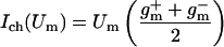1

where U_m,0 is the cell's resting potential (the offset from U_m = 0), I_c is a constant, w is the width of the sigmoid transition (Eq. 2) of g_m(U_m), and g and g are the minimum and maximum membrane conductances at very small and large U_m, respectively (g is the reciprocal of resistance). The resulting nonlinear U_m-dependent dynamic membrane conductance (Fig. 2 Right) has the form

2

The parameters had a fit value of w = 22 mV, and I_ch = 36 pA. The fixed membrane resistance is removed from I_ch(U_m) and shown separately as R_lip (Fig. 1), to be transparently consistent with traditional cell membrane models that contain explicit membrane resistance and capacitance. The data fit yields g = 8 pS and g = 9 nS (3 orders of magnitude larger with all channels open). For a cell membrane area ≈3 × 10⁻⁹ m² the value of g corresponds to a resistivity 7 × 10¹⁰ Ω m ≫ ρ_lip. In contrast, g corresponds to a membrane resistivity of 7 × 10⁷ Ω m.

Within an elementary area (ℓ²) the nonlinear dependence of current on U_m involves the entire population of ion channels and pumps and intra/extracellular ion concentration differences (33). In the cell models of Figs. 3 and 4 the magnitude of the nonlinear current source changes with position as U_m varies over the membrane because of electric field interactions involving the response field, E⃗_res. On a scale of ℓ², inhomogeneous channel distributions (14) can also be assigned over cell membranes as desired.

Membrane Electroporation Model.

A simple electroporation model is used in a time domain solution of the multicellular model (Fig. 5). A “square” pulse with a slew rate of 1,100 V⋅cm⁻¹⋅μs⁻¹ and pulse duration of 10 μs is applied. As U_m changes throughout the model, membrane sites reaching U_m >0.5 V make abrupt, irreversible downward transitions in resistance from ≈R_lip to R_m,[ep]. This finding corresponds to locally maximum permeabilization, consistent with 0.1% fractional aqueous area achieved during electroporation (34, 35).

Figure 5.

Effect of electroporation on equipotential (electric field) uniformity. (a–c) Time domain solutions for electroporation during a field pulse, E_app = 1,100 V⋅cm⁻¹ (leading edge rising at 1,100 V⋅cm¹⋅μs⁻¹). Red indicates electroporated membrane regions; elapsed time is shown in upper left corner. (d) All membranes maximally electroporated [0.1% area occupied by aqueous pores (34, 35)]. (e) Same as d, but supramaximally electroporated (1% aqueous area). (f–j) Equipotentials at 100 Hz for the corresponding cases of partial (at t = 1.8, 2.0, and 5.6 μs), maximal, and supramaximal electroporation.

Transport Lattice Solution.

Transport lattices (2D and 3D) are solved by Kirchhoff's laws, here using Berkeley spice version 3f5 (36, 37), yielding charges, currents, and voltages throughout the lattice. These quantities are available at any node or for any transport model element (e.g., U_m across M_m) and can be retrieved and then converted into quantities such as equipotentials (obtained by interpolation of nodal potentials), and SAR (dissipative power per mass within each elementary volume, ℓ³, using a mass density ρ_mass = 10³ kg⋅m⁻³). This step yields distributions of the traditional quantities φ, E⃗_res, U_m, J⃗, and SAR throughout the system model. Some of these quantities are displayed in Figs. 3–5, using matlab (Mathworks, Natick, MA). A single processor (1.2 GHz) computer with 1.5 gigabytes of memory, obtains solutions in 20 min (Figs. 4 and 5) to 8 h (Fig. 3).

Results and Discussion

A transport lattice is a system model that allows many features of a cellular system to be included. The geometry of one or more cells can be irregular, because idealized shapes are not needed to solve the electrical circuit that corresponds to the lattice. Moreover, the system model can have many regions of fluid, each with different properties. Many local interaction models can be included, with each elementary membrane area (ℓ²) assigned different models of membrane function. Here we assign four models (Fig. 1), keeping them identical at all cell membrane sites, with only the location, size, and shape of the cell varied (Fig. 4a). Nuclear membranes are included, but are assigned only fixed resistance and capacitance, consistent with previous models in which the nucleus is represented as a smaller concentric membrane within a spherical cell (8).

Kirchhoff's laws provide a fundamental description of charge transport along the localized paths that form the basis of electrical circuits (28). These laws ensure that currents entering and leaving nodes obey charge conservation and that the voltage drops around each closed path add up to zero. A system model is therefore a very large electrical circuit. A transport lattice provides an approximate, alternative approach to traditional analytical and finite element methods. This approach is consistent with earlier use of electrical analog computers to solve partial differential equations by using relatively small circuits (38). A transport lattice also allows both field-dependent transport (e.g., ionic conduction in aqueous electrolytes) and transmembrane voltage-dependent transport (e.g., voltage-gated channels and electroporation) to be easily incorporated into a system model. All of the local models interact, through paths that connect nearest neighbor local models. As computer power increases, the number of local models can be made larger, following the basic approach described here.

For comparison to analytical results (Fig. 3) we first treat the classic spherical cell model (3, 6–8, 29) by confining an approximately spherical membrane to a small volume. The low-frequency transmembrane voltage change at the sphere's poles for a high resistivity membrane is 0.99 times the analytical result, ΔU_m,pole = G_m,pole(0)E_appd_m = 1.5 E_appr_cell. This classic analytical prediction holds for an unconfined cell and infinitely distant electrodes (3, 6–8). The membrane area-averaged transmembrane voltage change squared is relevant to accumulated chemical change caused by periodic fields (7) and is 0.99 times the classic result, = 0.75 E_app²r_cell². The transport lattice region is somewhat larger than the cell (Fig. 3a) and therefore confines currents compared with an electrolyte of infinite extent. Cell confinement is a realistic condition for most in vivo tissues (15–18) and some in vitro systems (20–22). The transport lattice also has a finite number (here 1,218) of membrane sites where U_m is determined (Fig. 3b). For this reason our predictions yield slightly different transmembrane voltage changes than the analytic result.

The response field changes significantly with frequency. Below ≈100 kHz, E⃗_res is nearly excluded from the cell, whereas at ≈1 MHz the intracellular field is larger than the extracellular field over most of the cell. For 10–100 MHz the membrane impedance is negligible, and the larger intracellular resistivity is fully revealed (field inside larger than outside). However, for 1–10 GHz, E⃗_res is almost uniform throughout, making the cell almost “electrically invisible” (Fig. 3 c–h).

We also made predictions for a spherical cell model with the smaller membrane resistivity and dielectric properties of the intra- and extracellular electrolytes used recently by others (29) (Fig. 3). In this case, the field gain at the cell's poles, G_m,pole(f), agrees well with the second-order analytic model (29). Both models predict a large, frequency-independent gain from dc to ≈100 kHz, which is caused by conduction-dominated voltage division within the model (Fig. 3i). Both models also predict a nonzero field gain plateau for frequencies >≈300 MHz. This microwave frequency result is caused by dielectric-dominated voltage division. The slightly different predictions (Fig. 3i) arise mainly because the transport lattice region is finite, whereas the analytic model has infinite extent.

The multicellular system model results show that two basic types of field-amplifying mechanisms can exhibit frequency-dependent emergent behavior. Multiple cells can concentrate the current density, J⃗, and can therefore amplify E⃗_app to generate E⃗_res = ρJ⃗, increasing local SAR and thermal effects. Nonthermal interactions based on electroconformational mechanisms at the cell membrane (voltage-gated channels, field-sensitive enzymes, electroporation) involve position-dependent membrane field amplification gain, G_m(f), which can be regarded as voltage concentration.

Frequency-Dependent Amplification of E⃗_app by Current Density Concentration.

Consider the current density within the invagination of Fig. 4. As f increases from 100 Hz or less, the current density becomes increasingly concentrated within the invagination's electrolyte. In this sense E⃗_app is amplified, with E⃗_res increasing from almost zero at 100 Hz to appreciable values at higher frequencies (Fig. 4 c–h). Regions with concentrated J⃗ are apparent from examination of the blue equipotential lines. Closer line spacing corresponds to a larger E⃗_res and (for the same resistivity) larger J⃗. As frequency increases displacement currents increasingly flow across the membranes of cells lining the invagination and also across membranes of nearby cells. Thus, for time varying fields with high frequency components, invaginations can concentrate J⃗ and thereby amplify an applied field.

Below ≈300 MHz current density concentration also occurs within the cell layer gap (above site C), but involves pure conduction current that changes with frequency because of interactions throughout the system model. This causes elevated SAR (localized heating source; Fig. 4 i–m). Additional frequency-dependent distributions of fields are seen to emerge within and near the subendothelial cells that comprise the bulk of the model.

Above ≈300 MHz concentration of J⃗ by the multicellular system diminishes (Fig. 4n), the electric field becomes almost uniform (Fig. 4h), and emergent behavior is essentially lost. The response field approaches that of isolated cells (Fig. 3h), with the nearly uniform E⃗_res ≈ E⃗_app generating an extra- to intracellular SAR ratio close to ρ_e,in/ρ_e,ex (here a factor of 4). In this frequency range power dissipation is governed mainly by the electrolyte conductivity, with the largest heating in regions with the smallest conductivity (here extracellular fluid; Fig. 4n). These current density concentration responses are not quantitatively foreseen by isolated single-cell models.

Frequency-Dependent Amplification of E⃗_app by Voltage Concentration.

Voltage concentration occurs mainly across cell membranes. The membrane field gain, G_m(f), has four frequency regions, shown here for six illustrative membrane sites (Fig. 4b). Region I is defined by low-frequency plateaus in G_m(f). Conductive voltage division throughout the model results in a wide range of G_m(f) plateaus, with membrane sites at the invagination and parts of the tight cell layer achieving the largest values. These are examples of preferred sites for transmembrane voltage-based interactions.

Region II exhibits complicated emergent behavior, through a cell interacting with other groups of cells. For deeper cells (sites D, E, and F) maximum shielding of some cells from electric fields occurs in region I, with frequency-dependent partial loss of shielding arising in region II. Within regions II and III some membrane sites experience broad peaks in G_m(f) (sites D, E, and F). Frequency ranges with enhanced responses have been termed “windows,” but often lack a theoretical basis (8). Cells within the cell layer with tight junctions (sites A and B) or near the cell layer gap (site C) experience decreasing G_m(f) in region II. In region III cells have monotonic decreases in G_m(f), also a feature of the isolated spherical cell. As microwave frequencies are reached in region IV there are smooth transitions of G_m(f) into small plateaus governed by dielectric voltage division, with G_m(f) dropping from maximum values of ≈10⁴ in region I to ≈10 or less in region IV. The complicated behavior of voltage concentration at cell membrane sites is caused by distributed interactions involving the entire multicellular system. For a given site, nearby cells and more distant layers of cells with tight junctions are particularly important.

Very large G_m(f) that is achieved by very large and specialized multicellular structures is fundamental to detection of weak dc and extremely low-frequency fields. The ampullae of Lorenzini in elasmobranch fish concentrate a whole body voltage to two layers of specialized cells (4, 9). The relatively small nonspecialized multicellular invagination of Fig. 4 leads to much smaller but nevertheless significant membrane amplification at low frequencies for some cells, but this is essentially lost at microwave frequencies.

Electroporation and Electric Field Inhomogeneities.

Time domain electrical responses also exhibit emergent behavior. We consider electroporation, which is a nonthermal effect that nonlinearly depends on U_m and involves voltage concentration (8, 35). Electroporation is shown here to be favored at sites near an invagination and a cell layer gap (Fig. 5). The spatial distribution of electroporation is predicted during a pulse of magnitude E⃗_app = 1,100 V⋅cm⁻¹, typical for small molecule delivery in vivo (18). For this pulse the electroporation distribution stops growing within ≈5 μs. Unlike the smooth electroporated polar region of a large, isolated spherical cell (34) electroporation in the multicellular model is highly nonuniform. A complex pattern of electropermeabilized cell membrane regions develops, preferentially in and near the cell layer, and near the gap in the layer. Such heterogeneity is relevant to in vivo electroporation (16, 18, 39).

The greatly decreased resistance of electroporated membranes does not create a homogeneous E⃗_res (compare the 100-Hz equipotentials of Figs. 4c and 5 a–c). Even if all cell membranes were extensively electroporated emergent behavior persists (Fig. 5 d and e). This result supports the view that achieving a homogeneous electrical response below microwave frequencies is extremely difficult in multicellular systems.

Microwaves are indeed extremely effective in generating a nearly homogeneous response in a multicellular system with nonelectroporated cells (Fig. 4h), almost eliminating significant field amplification. This conclusion is relevant to reported nonthermal effects in a multicellular organism at microwave frequencies (12) and the use of magnetic resonance imaging with very strong magnetic fields that involve Larmour frequencies ≥300 MHz. Subcellular structures, particularly magnetosomes (40), create small inhomogeneities on a length scale of their size (≈0.1 μm), which is much smaller than typical mammalian cells and therefore insignificant on a multicellular scale.

Together our results illustrate the importance of considering multicellular models for the response of biological systems to electric fields. Predicting electrical quantities is a necessary first step for estimating field-induced chemical changes (7, 9, 27, 41, 42) that will be needed to achieve a comprehensive understanding of interactions of electric fields with cellular systems. Transport lattice models of cellular systems for heat transport and molecular and ionic transport are also possible and can be used in combination with an electrical transport lattice model to approach more general cell modeling problems. As illustrated here, one goal of cellular system models can be creation of models for small (Fig. 4) to large (Fig. 5) electric fields by using a single system model. The multicellular model shows that some cells may experience thermal effects through localized heating associated with current density concentration. Other cells may have nonthermal effects through voltage concentration that favors transmembrane voltage-dependent interactions (channel gating, electroconformational coupling, electroporation). Both types of responses can involve the interaction of many cells. Cell models based on transport lattices are a restricted subset of complex networks (36, 43), with only nearest neighbor connections. Their essential feature is prediction based on the interaction of many local transport models within a system model.

Abbreviation

SAR

specific absorption rate

References

- 1.Levin M, Thorlin T, Robinson K R, Nogi T, Mercola M. Cell. 2002;111:77–89. doi: 10.1016/s0092-8674(02)00939-x. [DOI] [PubMed] [Google Scholar]
- 2.Song B, Zhao M, Forrester J V, McCaig C D. Proc Natl Acad Sci USA. 2002;99:13577–13582. doi: 10.1073/pnas.202235299. [DOI] [PMC free article] [PubMed] [Google Scholar]
- 3.Pauly H, Schwan H P. Z Naturforsch B. 1959;14:125–131. [PubMed] [Google Scholar]
- 4.Kalmijn A J. Science. 1982;218:916–918. doi: 10.1126/science.7134985. [DOI] [PubMed] [Google Scholar]
- 5.McLeod K J, Lee R C, Ehrlich H P. Science. 1987;236:1465–1469. doi: 10.1126/science.3589667. [DOI] [PubMed] [Google Scholar]
- 6.Weaver J C, Astumian R D. Science. 1990;247:459–462. doi: 10.1126/science.2300806. [DOI] [PubMed] [Google Scholar]
- 7.Astumian R D, Weaver J C, Adair R K. Proc Natl Acad Sci USA. 1995;92:3740–3743. doi: 10.1073/pnas.92.9.3740. [DOI] [PMC free article] [PubMed] [Google Scholar]
- 8.Polk C, Postow E, editors. CRC Handbook of Biological Effects of Electromagnetic Fields. 2nd Ed. Boca Raton, FL: CRC; 1996. [Google Scholar]
- 9.Adair R K, Astumian R D, Weaver J C. Chaos. 1998;8:576–587. doi: 10.1063/1.166339. [DOI] [PubMed] [Google Scholar]
- 10.Segev I, London M. Science. 2000;290:744–750. doi: 10.1126/science.290.5492.744. [DOI] [PubMed] [Google Scholar]
- 11.Sohn L L, Salch O A, Facer G R, Beavis A J, Allan R S, Notterman D A. Proc Natl Acad Sci USA. 2000;26:10687–10690. doi: 10.1073/pnas.200361297. [DOI] [PMC free article] [PubMed] [Google Scholar]
- 12.de Pomerai D, Daniells C, David H, Allan J, Duce I, Mutwakil M, Thomas D, Sewell P, Tattersall J, Jones D, Candido P. Nature. 2000;405:417–418. doi: 10.1038/35013144. [DOI] [PubMed] [Google Scholar]
- 13.Aidley D J. The Physiology of Excitable Cells. 4th Ed. Cambridge, U.K.: Cambridge Univ. Press; 1998. [Google Scholar]
- 14.Hille B. Ionic Channels of Excitable Membranes. 3rd Ed. Sunderland, MA: Sinauer; 2001. [Google Scholar]
- 15.Lee R C, River L P, Pan F-S, Ji L, Wollmann R L. Proc Natl Acad Sci USA. 1992;89:4524–4528. doi: 10.1073/pnas.89.10.4524. [DOI] [PMC free article] [PubMed] [Google Scholar]
- 16.Prausnitz M R, Bose V G, Langer R, Weaver J C. Proc Natl Acad Sci USA. 1993;90:10504–10508. doi: 10.1073/pnas.90.22.10504. [DOI] [PMC free article] [PubMed] [Google Scholar]
- 17.Mir L M, Bureau M F, Gehl J, Rangara R, Rouy D, Caillaud J-M, Delaere P, Brannellec D, Schwarts B, Scherman D. Proc Natl Acad Sci USA. 1999;96:4262–4267. doi: 10.1073/pnas.96.8.4262. [DOI] [PMC free article] [PubMed] [Google Scholar]
- 18.Jaroszeski M J, Gilbert R, Heller R, editors. Electrically Mediated Delivery of Molecules to Cells: Electrochemotherapy, Electrogenetherapy, and Transdermal Delivery by Electroporation. Totowa, NJ: Humana; 2000. [Google Scholar]
- 19.Golzio M, Teissie J, Rols M P. Proc Natl Acad Sci USA. 2002;99:1292–1297. doi: 10.1073/pnas.022646499. [DOI] [PMC free article] [PubMed] [Google Scholar]
- 20.Lundqvist J A, Sahlin F, Aberg M A, Stromberg A, Eriksson P S, Orwar O. Proc Natl Acad Sci USA. 1998;95:10356–10360. doi: 10.1073/pnas.95.18.10356. [DOI] [PMC free article] [PubMed] [Google Scholar]
- 21.Huang Y, Rubinsky B. Biomed Microdevices. 1999;2:145–150. [Google Scholar]
- 22.Strömberg A, Ryttsén F, Chiu D T, Davidson M, Eriksson P S, Wilson C F, Orwar O, Zare R N. Proc Natl Acad Sci USA. 2000;97:7–11. doi: 10.1073/pnas.97.1.7. [DOI] [PMC free article] [PubMed] [Google Scholar]
- 23.Schoenbach K H, Beebe S J, Buescher E S. Bioelectromagnetics. 2001;22:440–448. doi: 10.1002/bem.71. [DOI] [PubMed] [Google Scholar]
- 24.Zeira M, Tosi P-F, Mouneimne Y, Lazarte J, Sneed L, Volsky D J, Nicolau C. Proc Natl Acad Sci USA. 1991;88:4409–4413. doi: 10.1073/pnas.88.10.4409. [DOI] [PMC free article] [PubMed] [Google Scholar]
- 25.Tsong T Y, Astumian R D. Annu Rev Physiol. 1988;50:273–290. doi: 10.1146/annurev.ph.50.030188.001421. [DOI] [PubMed] [Google Scholar]
- 26.Neumann E, Sowers A E, Jordan C A, editors. Electroporation and Electrofusion in Cell Biology. New York: Plenum; 1989. [Google Scholar]
- 27.Chang D C, Chassy B M, Saunders J A, Sowers A E, editors. Guide to Electroporation and Electrofusion. New York: Academic; 1992. [Google Scholar]
- 28.Benedek G B, Villars F M H. Physics with Illustrative Examples from Medicine and Biology. 2nd Ed. Vol. 3. New York: Am. Institute of Physics; 2000. [Google Scholar]
- 29.Kotnik T, Miklavèiè D. IEEE Trans Biomed Eng. 2000;47:1074–1081. doi: 10.1109/10.855935. [DOI] [PubMed] [Google Scholar]
- 30.Fear E C, Stuchly M A. IEEE Trans Biomed Eng. 1998;45:856–866. doi: 10.1109/10.686793. [DOI] [PubMed] [Google Scholar]
- 31.Mudd C. J Biochem Biophys Methods. 1999;39:7–38. doi: 10.1016/s0165-022x(98)00045-1. [DOI] [PubMed] [Google Scholar]
- 32.Blakely R D, DeFelice L J, Hartzell H C. J Exp Biol. 1994;196:263–281. doi: 10.1242/jeb.196.1.263. [DOI] [PubMed] [Google Scholar]
- 33.Läuger P. Electrogenic Ion Pumps. Sunderland, MA: Sinauer; 1991. [Google Scholar]
- 34.Hibino M, Shigemori M, Itoh H, Nagyama K, Kinosita K. Biophys J. 1991;59:209–220. doi: 10.1016/S0006-3495(91)82212-3. [DOI] [PMC free article] [PubMed] [Google Scholar]
- 35.Freeman S A, Wang M A, Weaver J C. Biophys J. 1994;67:42–56. doi: 10.1016/S0006-3495(94)80453-9. [DOI] [PMC free article] [PubMed] [Google Scholar]
- 36.Mikulecky D C. Applications of Network Thermodynamics to Problems in Biomedical Engineering. New York: New York Univ. Press; 1993. [Google Scholar]
- 37.Vladimirescu A. The SPICE Book. New York: Wiley; 1994. [Google Scholar]
- 38.Kron G. J Appl Phys. 1945;16:172–186. [Google Scholar]
- 39.Gaylor D C, Prakah-Asante K, Lee R C. J Theor Biol. 1988;133:223–237. doi: 10.1016/s0022-5193(88)80007-9. [DOI] [PubMed] [Google Scholar]
- 40.Kirschvink J L, Kirschvink A K, Woodford B J. Proc Natl Acad Sci USA. 1992;89:7683–7687. doi: 10.1073/pnas.89.16.7683. [DOI] [PMC free article] [PubMed] [Google Scholar]
- 41.Weaver J C, Vaughan T E, Martin G T. Biophys J. 1999;76:3026–3030. doi: 10.1016/S0006-3495(99)77455-2. [DOI] [PMC free article] [PubMed] [Google Scholar]
- 42.Weaver J C. Bioelectrochemistry. 2002;56:207–209. doi: 10.1016/s1567-5394(02)00038-5. [DOI] [PubMed] [Google Scholar]
- 43.Strogatz S H. Nature. 2001;410:268–276. doi: 10.1038/35065725. [DOI] [PubMed] [Google Scholar]