Amino acid empirical contact energy definitions for fold recognition in the space of contact maps

Abstract

Background

Contradicting evidence has been presented in the literature concerning the effectiveness of empirical contact energies for fold recognition. Empirical contact energies are calculated on the basis of information available from selected protein structures, with respect to a defined reference state, according to the quasi-chemical approximation. Protein-solvent interactions are estimated from residue solvent accessibility.

Results

In the approach presented here, contact energies are derived from the potential of mean force theory, several definitions of contact are examined and their performance in fold recognition is evaluated on sets of decoy structures. The best definition of contact is tested, on a more realistic scenario, on all predictions including sidechains accepted in the CASP4 experiment. In 30 out of 35 cases the native structure is correctly recognized and best predictions are usually found among the 10 lowest energy predictions.

Conclusion

The definition of contact based on van der Waals radii of alpha carbon and side chain heavy atoms is seen to perform better than other definitions involving only alpha carbons, only beta carbons, all heavy atoms or only backbone atoms. An important prerequisite for the applicability of the approach is that the protein structure under study should not exhibit anomalous solvent accessibility, compared to soluble proteins whose structure is deposited in the Protein Data Bank. The combined evaluation of a solvent accessibility parameter and contact energy allows for an effective gross screening of predictive models.

Background

Renewed interest in the protein folding problem has been stimulated by both the boost in genomic projects and by continuous improvement in prediction achievements.

A wide range of tools has been employed for structure prediction ranging from coarse grained lattice representations to all atoms molecular dynamics simulations [1,2].

A guiding principle of most prediction models is that protein native structure is thermodynamically stable and therefore it is at a free energy minimum [3]. As a consequence, the problem of finding the native structure can be split in two main components:

i) the representation of a protein by a model which allows the definition of a (free) energy for each of its conformations;

ii) the development of an efficient search algorithm.

Very different empirical functions have been previously defined (see for a review ref. [4]), and their ability in discriminating the native structure from non-native ones has been explored for different proteins, also in comparative studies [5].

One model which has attracted much interest describes, in a very compact way, protein conformation using residue-residue contact maps: for each residue pair a Boolean variable is introduced which describes the presence or absence of a contact. It has been shown that with a sufficient number of contacts, protein structure can be reconstructed with sufficient accuracy (see e.g. ref. [6]).

To each amino acid pair in contact an (additive) energy is assigned and the energy of the protein can be estimated from the sum of all pairwise energies.

Empirical contact energies may be derived in different ways, mainly employing optimisation algorithms that maximise the gap between the free energy assigned to the native and decoy structures, or statistical survey of contacts in native structures.

In the present work, empirical energies are calculated using the statistical information derived from an ensemble of protein structures, selected from a structural database, and should reflect the propensity of each amino acid type to interact with any other amino acid type. The performance of the method depends on model definition and the present investigation aims at evaluating different models and at establishing applicability limits of the model itself.

The first attempt to calculate empirical contact energy, from structural information available from a dedicated data base, is attributable to Tanaka and Scheraga [7] and it was later developed by Miyazawa and Jernigan [8-11].

Empirical contact energies may be used in fold recognition experiments, where a contact matrix represents a protein conformation. This approach has the drawback that it is not easy to discriminate against unphysical contact maps, although some heuristic rules have been defined to solve this problem [6,12,13]. A solution to this problem can be the use of additive energetic terms, such as the repulsion energy term, as formulated by Miyazawa and Jernigan [9], and local conformational propensity energy terms.

Following the work of Miyazawa and Jernigan, many new ideas and improvements, such as the choice of a different reference state [14,15], or of a different amino acid's representation [14,16,17], have been proposed in recent years.

Notwithstanding all the criticisms received, in particular concerning the non-additivity of contact potentials ([18] and see ref. [19] for a general discussion on a related issue) the quasi-chemical approximation seems to perform generally satisfactorily [9].

As far as protein representation is concerned, several models have been used and Park and Levitt [5] examined and compared the performance of several different contact and energy definitions, showing that a combination of different energy functions is able to discriminate the native structure from decoys. Vendruscolo et al. [20] investigated the possibility itself of defining contact energies able to discriminate native from decoy structures with a general negative answer.

As far as the search algorithm for the contact map model is concerned the main problem is that only a limited number of plausible contact maps are physically feasible, because of stereochemical constraints on amino acid conformations. Moreover the energy definition based on contacts does not take into account other local conformational preferences, like secondary structure propensities, which are of fundamental importance for protein structure. Search algorithms must take into account all these aspects as done for instance by the algorithm of Vendruscolo and Domany [12] which aims at generating only physically feasible conformations. Prediction of contacts from sequence is still difficult although there have been improvements in the last years [21,22]. All results obtained on decoys should, in view of these problems, taken with much care. In this respect predictions made in the Critical Assessment of Structure Prediction (CASP) experiment [23] should be more realistic as these make usually use of alignment, homology modeling and threading on real structures.

In the present work we investigate the reliability of amino acid empirical contact energy definitions for use in fold recognition, by searching and testing the optimal definition of contact. In the Methods section the theory underlying the present approach is presented. Compared to the method of Miyazawa and Jernigan [8,9], the present derivation is somewhat simpler, it is based on the potential of mean force theory and relies (in a simple way) only on contact counts and solvent accessibility.

Results

Solvent accessibility parameter

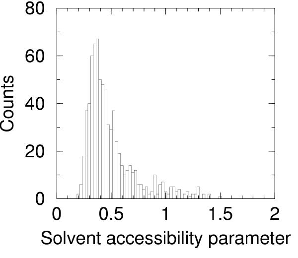
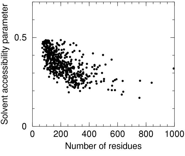
The solvent accessibility parameter defined in the Materials and methods section has been computed for all the 746 chains in the dataset of proteins selected from the pdb_select ensemble. The distribution of the solvent accessibility parameter is reported as a histogram in Figure 1. The largest values refer mainly to short chains in association with other larger units or in some cases to proteins classified as membrane proteins. After selection of 500 proteins with the lowest values of solvent accesibility parameter (less than 0.486) a weak anti-correlation of the solvent accessibility parameter with the number of residues is found, as can be gleaned from Figure 2. It is likely that very large values of this parameter for predictive models will hint at some problems with the model or be indicative of association with other units.

Figure 1.

Histogram of solvent accessibility parameter The histogram (bin width 0.025) of solvent accessibility parameter computed on the 746 proteins selected from the pdb_select 25%.

Figure 2.

Solvent accessibility parameter versus number of residues The solvent accessibility parameter is plotted versus the number of residues for the 500 proteins with solvent accessibility parameter values lower than 0.486 (see text).

Optimal contact definition

The discrimination performance for different contact definitions was estimated by means of the z-score and the rank score (see Methods section). In particular several cutoff values were tested using the following different residue-residue distance definitions:

i) the distance between alpha carbons (CA);

ii) the distance between beta carbons, or alpha carbon for glycine (CB);

iii) the minimum distance between the van der Waals spheres of each residue heavy atoms (HA);

iv) the minimum distance between the van der Waals spheres of each residue backbone heavy atoms (BB);

v) the minimum distance between the van der Waals spheres of each residue side chain heavy atoms or alpha carbons (SC+CA);

For all these definitions empirical contact energies have been derived from contacts observed in the dataset. Then, for each sequence in the dataset, energies corresponding to all matrices were computed and used to obtain a distribution of energy values. From this distribution of values the z-score and the rank score corresponding to the native structure could be estimated. The results are reported in Table 1 where the mean z-scores corresponding to each distance definition are reported versus the cutoff value. In all cases, except for the worst choices the rank score was 1.

Table 1.

Test of different contact definitions on the dataset

Cutoff (Å)	All atoms	SC+CA	BB	CB	CA
0.4	2.15	5.53	0.05	-	-
0.5	2.14	7.08	0.10	-	-
0.6	2.21	7.33	0.22	0.03	-
0.7	2.28	6.85	0.49	0.03	-
0.8	2.36	6.31	1.03	0.03	-0.02
0.9	2.43	5.82	1.52	0.03	-0.05
1.0	2.49	5.44	1.63	0.05	-0.07
1.1	2.56	5.16	1.59	0.08	-0.06
1.2	2.59	4.93	1.53	0.12	-0.05
1.3	2.61	4.76	1.49	0.15	-0.04
1.4	2.61	4.63	1.46	0.21	-0.03
1.6	-	-	-	0.37	0.07
1.8	-	-	-	0.72	0.08
2.0	-	-	-	1.50	0.14
2.2	-	-	-	3.07	0.62
2.4	-	-	-	4.18	1.53
2.6	-	-	-	4.09	1.95
2.8	-	-	-	3.74	1.80

The average z-score (see Materials and methods section) for different contact definitions is reported versus the cutoff employed.

From Table 1 it is apparent that the SC+CA distance definition is the best performing one, because mean z-score values are clearly higher. The same results prove that the definition of residue-residue distance is a crucial determinant of the discrimination performance of empirical contact energies.

It should also be noted that, as expected, when the information deriving from side chains is ignored and only backbone's atoms are considered, the system is characterised by very poor discrimination power. A somewhat unexpected result is that ignoring backbone atoms improves discrimination performance. We ascribe this behaviour to rather unspecific information provided by backbone atoms.

In this analysis, the discrimination system was tested on the same proteins employed for the empirical energies calculation.

Before proceeding further, these conclusions have been tested more rigorously on few proteins not belonging to the proteins' dataset with similar results. Optimal cutoff values for these few tested proteins were in the range 0.7 to 0.9 Å.

Fold recognition experiments on decoys' sets

In view of the rather crude derivation of optimal contact definition we tested and refined it on alternatives generated by predictive computational methods: these alternative conformations are called decoys. Many decoys' sets are available, and they differ from one another in the protein to which they refer, and, more important, in the algorithm producing them.

Because of the previous observations, the SC+CA distance definition was employed and cutoff's value was separately set at 0.7 Å, 0.8 Å, 0.9 Å, 1.0 Å, 1.1 Å, 1.2 Å, 1.3 Å and 1.4 Å. For every tested protein, the reference structure deposited in the PDB [24] was always considered as the native conformation. The fold recognition performance was tested using both the rank score and z-score.

For all the proteins in the misfold set the native conformation was assigned the lower energy, thus allowing the discrimination against the alternative structure. The misfold set has been generated a decade ago by Holm and Sander [25] by superimposing the sequence of a protein on the structure of another. Although this might seem a very rough procedure it is worth mentioning that not all methods reported in the literature recognize the native fold for all protein pairs, probably due to missing heterogroups (see e.g. [26-28]).

A more challenging test has been conducted with the other three sets of decoys, because they offer many alternative non-native conformations. Results are summarised in Table 2. The discrimination performance, judged by z-score and rank score, critically depends on the solvent accessibility parameter and on the number of residues in the chain. It is, in fact, important to note that worst performance is found for the shortest chains, namely with lengths 31, 36 and 43 amino acids, and for proteins with the highest solvent accessibility parameter, which indicates that the protein cannot be described by the assumed model itself.

Table 2.

Performance of contact energies for fold recognition

4state
Protein Cutoff (Å)	1ctf z-score	rank	1r69z-score	rank	1sn3z-score	rank	2cro z-score	rank	3icb z-score	rank	4pti z-score	rank	4rxn z-score	rank
0.7	3.24	1	5.07	1	3.32	1	3.54	1	2.95	1	4.86	1	5.40	1
0.8	3.43	1	5.35	1	3.68	1	4.65	1	3.03	1	5.30	1	5.68	1
0.9	3.80	1	5.43	1	3.49	1	4.55	1	3.37	1	4.90	1	5.50	1
1.0	4.21	1	5.39	1	3.60	1	4.81	1	3.22	1	5.03	1	5.28	1
1.1	4.50	1	5.89	1	3.71	1	5.11	1	3.00	1	4.84	1	5.49	1
1.2	4.83	1	5.90	1	3.47	1	5.11	1	3.01	1	4.77	1	5.40	1
1.3	4.53	1	5.58	1	3.31	1	4.76	1	2.79	1	4.56	1	5.12	1
1.3	4.09	1	5.06	1	3.16	1	4.29	1	3.23	1	4.52	1	4.81	1
acc. par.	0.39		0.44		0.54		0.49		0.37		0.53		0.58
length	68		63		65		65		75		58		54
casp3
Protein Cutoff (Å)	1bg8-A z-score	rank	1bl0z-score	rank	1eh2z-score	rank	1jwe z-score	rank
0.7	2.78	4	-0.01	486	2.74	12	2.48	12
0.8	3.16	1	0.10	455	2.95	4	3.70	1
0.9	3.38	1	0.73	223	2.82	4	4.36	1
1.0	3.61	1	1.03	151	3.09	2	4.54	1
1.1	3.92	1	1.07	70	3.35	2	4.35	1
1.2	3.35	1	1.02	80	3.56	2	4.09	1
1.3	3.01	1	0.67	134	3.26	3	3.80	1
1.4	2.88	1	0.80	107	3.11	4	3.59	1
acc. par.	0.55		0.40		0.48		0.46
length	76		99		79		114
lmds
Protein Cutoff (Å)	1b0n-B z-score	rank	1bba z-score	rank	1fc2z-score	rank
0.7	1.11	76	1.02	65	-5.76	501
0.8	0.54	153	0.44	163	-5.44	501
0.9	0.79	116	-0.07	264	-5.04	501
1.0	0.58	148	-0.84	395	-5.25	501
1.1	1.15	59	-1.42	457	-4.74	501
1.2	1.53	35	-1.53	472	-4.36	501
1.3	1.63	29	-1.19	442	-4.89	501
1.4	1.42	40	-1.05	424	-3.77	501
acc. par.	1.08		0.83		0.57
length	31		36		43
lmds
Protein Cutoff (Å)	1ctf z-score	rank	1dtk z-score	rank	1igd z-score	rank	1shf-A z-score	rank	2cro z-score	rank	2ovo z-score	rank	4pti z-score	rank
0.7	2.89	1	1.44	16	3.48	1	3.19	1	3.69	1	1.88	14	2.76	5
0.8	3.24	1	1.32	20	3.97	1	4.90	1	5.73	1	1.84	16	3.38	3
0.9	3.64	1	1.57	11	3.94	1	4.77	1	6.12	1	2.30	6	3.17	4
1.0	4.17	1	2.50	3	3.84	1	4.56	1	6.91	1	2.47	6	3.51	1
1.1	4.60	1	3.39	1	4.06	1	4.59	1	7.63	1	2.27	7	3.40	2
1.2	4.86	1	3.18	1	3.51	1	4.99	1	7.84	1	2.35	8	3.54	2
1.3	4.72	1	3.53	1	3.24	2	4.77	1	7.58	1	2.31	6	3.52	2
1.4	4.42	1	3.26	1	3.26	1	4.37	1	7.17	1	2.46	5	3.64	1
acc. par.	0.39		0.55		0.56		0.58		0.49		0.66		0.52
length	68		63		65		65		75		58		54

For all the tested decoys' sets the z-score and the rank score are reported for the SC+CA contact definition. The number of residues for each chain and the solvent accessibility parameter are also reported.

Another important point is that the highest discrimination performance is not always achieved with the same cutoff value. This fact could be due to different ways of producing the decoys' sets. Nevertheless, even in different decoys' sets belonging to the same group, i. e. constructed using the same algorithm, a single cutoff value is not always the best one. So other effects should be responsible for the discrimination performance.

Best discrimination is obtained for cutoffs in the range 1.0 – 1.3 Å, as opposed to much shorter optimal cutoff in the gross test performed on the dataset sequences.

Amongst short chains, a singular behavior is observed for 1fc2, whose native structure is always associated to the highest energy. This result is fully consistent with the results of Felts et. al. [29]. An explanation for this unexpected behaviour is that the chain is a fragment of a larger chain (protein A) which is associated in the PDB file with another protein (a FC fragment) and model assumptions are not respected in this case.

Unfavourable results were obtained in the case of 1bl0 protein, whose rank score value was 151 (with cutoff 1.0 Å), in spite of the acceptable solvent accessibility parameter value. If all decoys were ordered with respect to the estimated energy, in the first 25 alternative conformations, 13 structures with RMSD greater than 13 Å, calculated with respect to the native structure, are found (Figure 3). It should be however mentioned that the RMSD among these 13 structures is in the range 0.5 to 1.0 Å.

Figure 3.

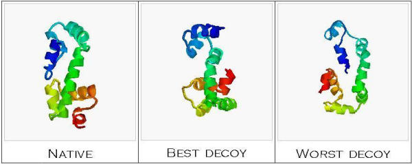
1bl0 structure and decoys The native structure of multiple antibiotic resistance protein (pdb id. 1bl0) is shown together with the best decoy (i.e. the lowest energy) decoy and the worst decoy (i.e. the highest energy decoy).

Structure 1bl0 represents a multiple antibiotic resistance protein interacting with a DNA molecule through a wide portion of its exposed surface [30] this fact may be important because the environment could not be treated as it was completely aqueous solvent.

This and the previous examples show that our simple solvent accessibility parameter, although useful, could not be sufficient to ascertain the infringement or observance of model's limitations.

It is interesting to note, however, that, for a few tested proteins for which both free and complexed structures are available in the PDB, the energy associated to the free conformation was found to be lower than that of the bound conformation for three tested proteins.

Empirical contact energies

The calculated energies for a dehydration reaction, with the SC+CA contact definition and cutoff value 1.0 Å, are reported in Table 3. The cutoff value has been chosen as a reasonable average in view of results obtained in the tests on the dataset obtained by gapless threading and on the decoys' sets.

Table 3.

Amino acid empirical contact energies

	CYS	MET	PHE	ILE	LEU	VAL	TRP	TYR	ALA	GLY
CYS	-3.477	-2.240	-2.424	-2.410	-2.343	-2.258	-2.080	-1.892	-1.700	-1.101
MET	-2.240	-1.901	-2.304	-2.286	-2.208	-2.079	-2.090	-1.834	-1.517	-0.897
PHE	-2.424	-2.304	-2.467	-2.530	-2.491	-2.391	-2.286	-1.963	-1.750	-1.034
ILE	-2.410	-2.286	-2.530	-2.691	-2.647	-2.568	-2.303	-1.998	-1.872	-0.885
LEU	-2.343	-2.208	-2.491	-2.647	-2.501	-2.447	-2.222	-1.919	-1.728	-0.767
VAL	-2.258	-2.079	-2.391	-2.568	-2.447	-2.385	-2.097	-1.790	-1.731	-0.756
TRP	-2.080	-2.090	-2.286	-2.303	-2.222	-2.097	-1.867	-1.834	-1.565	-1.142
TYR	-1.892	-1.834	-1.963	-1.998	-1.919	-1.790	-1.834	-1.335	-1.318	-0.818
ALA	-1.700	-1.517	-1.750	-1.872	-1.728	-1.731	-1.565	-1.318	-1.119	-0.290
GLY	-1.101	-0.897	-1.034	-0.885	-0.767	-0.756	-1.142	-0.818	-0.290	0.219
THR	-1.243	-0.999	-1.237	-1.360	-1.202	-1.240	-1.077	-0.892	-0.717	-0.311
SER	-1.306	-0.893	-1.178	-1.037	-0.959	-0.933	-1.145	-0.859	-0.607	-0.261
ASN	-0.788	-0.658	-0.790	-0.669	-0.524	-0.673	-0.884	-0.670	-0.371	-0.230
GLN	-0.835	-0.720	-0.807	-0.778	-0.729	-0.642	-0.997	-0.687	-0.323	0.033
ASP	-0.616	-0.409	-0.482	-0.402	-0.291	-0.298	-0.613	-0.631	-0.235	-0.097
GLU	-0.179	-0.209	-0.419	-0.439	-0.366	-0.335	-0.624	-0.453	-0.039	0.443
HIS	-1.499	-1.252	-1.330	-1.234	-1.176	-1.118	-1.383	-1.222	-0.646	-0.325
ARG	-0.771	-0.611	-0.805	-0.854	-0.758	-0.664	-0.912	-0.745	-0.327	-0.050
LYS	-0.112	-0.146	-0.270	-0.253	-0.222	-0.200	-0.391	-0.349	0.196	0.589
PRO	-1.196	-0.788	-1.076	-0.991	-0.771	-0.886	-1.278	-1.067	-0.374	-0.042
	THR	SER	ASN	GLN	ASP	GLU	HIS	ARG	LYS	PRO
CYS	-1.243	-1.306	-0.788	-0.835	-0.616	-0.179	-1.499	-0.771	-0.112	-1.196
MET	-0.999	-0.893	-0.658	-0.720	-0.409	-0.209	-1.252	-0.611	-0.146	-0.788
PHE	-1.237	-1.178	-0.790	-0.807	-0.482	-0.419	-1.330	-0.805	-0.270	-1.076
ILE	-1.360	-1.037	-0.669	-0.778	-0.402	-0.439	-1.234	-0.854	-0.253	-0.991
LEU	-1.202	-0.959	-0.524	-0.729	-0.291	-0.366	-1.176	-0.758	-0.222	-0.771
VAL	-1.240	-0.933	-0.673	-0.642	-0.298	-0.335	-1.118	-0.664	-0.200	-0.886
TRP	-1.077	-1.145	-0.884	-0.997	-0.613	-0.624	-1.383	-0.912	-0.391	-1.278
TYR	-0.892	-0.859	-0.670	-0.687	-0.631	-0.453	-1.222	-0.745	-0.349	-1.067
ALA	-0.717	-0.607	-0.371	-0.323	-0.235	-0.039	-0.646	-0.327	0.196	-0.374
GLY	-0.311	-0.261	-0.230	0.033	-0.097	0.443	-0.325	-0.050	0.589	-0.042
THR	-0.617	-0.548	-0.463	-0.342	-0.382	-0.192	-0.720	-0.247	0.155	-0.222
SER	-0.548	-0.519	-0.423	-0.260	-0.521	-0.161	-0.639	-0.264	0.223	-0.199
ASN	-0.463	-0.423	-0.367	-0.253	-0.344	0.160	-0.455	-0.114	0.271	-0.018
GLN	-0.342	-0.260	-0.253	0.054	0.022	0.179	-0.290	-0.042	0.334	-0.035
ASP	-0.382	-0.521	-0.344	0.022	0.179	0.634	-0.664	-0.584	-0.176	0.189
GLU	-0.192	-0.161	0.160	0.179	0.634	0.933	-0.324	-0.374	-0.057	0.257
HIS	-0.720	-0.639	-0.455	-0.290	-0.664	-0.324	-1.078	-0.307	0.388	-0.346
ARG	-0.247	-0.264	-0.114	-0.042	-0.584	-0.374	-0.307	0.200	0.815	-0.023
LYS	0.155	0.223	0.271	0.334	-0.176	-0.057	0.388	0.815	1.339	0.661
PRO	-0.222	-0.199	-0.018	-0.035	0.189	0.257	-0.346	-0.023	0.661	0.129

Contact energies are reported for all amino acid pairs corresponding to the SC+CA contact definition and employing a cutoff of 1.0 Å.

The lowest energy value correspond to the contact between cysteines, which reflects the unique capability of cysteines of forming disulphide bridges. This feature was found also by other authors, following different schemes (see e.g. ref. [9]).

Consistently with similar studies, very low energy values can be observed, as expected, for contacts between hydrophobic residues, while unfavourable energies regard the formation of contacts involving residues with electrostatic charge of the same sign. The preference of polar residues for contacts with other polar residues or solvent is much less pronounced, thus confirming the main role of the hydrophobic effect in protein stability.

Analysis of the results on the 4state decoys' set

The results obtained on decoys and summarized in Table 2 give a good impression of the performance of the methodology. However it is worth reminding that the task of recognizing an experimental structure among a set decoys is poorly related to real fold recognition tasks. First of all in a real fold recognition experiment the task is to recognize, among several predictive models, native-like structures, rather than native structure, whose overall RMSD with the native structure can be rather high (say e.g. ca. 5 Å). For this reason it is very important that any energy function should show some correlation with the RMSD of the predictive models from native structure.

Second a native-like structure could not be present in the ensemble and we should be able to recognize this fact, either at the gross test stage or at a later stage.

Third, the specific environment, or cofactors, or association state of the protein is often not known, and this can lead to discarding good structures, based, for instance on solvent accessibility properties, when a hydrophobic interface is not recognized as such.

The two latter issues can be better tested on blind predictions made in the context of the CASP experiment [23] and they will be addressed in the next section.

Concerning the first issue raised above, the 4state set of decoys was chosen for test because it has been generated by keeping most of the structure in native conformation, and choosing for just few "hinge" regions a set of allowed conformations [5]. The original paper by Park and Levitt [5] contains several analysis which allow comparison with the present results. An outstanding property of these decoys is that several near-native conformations exist and RMSDs are well distributed even at low values. The procedure used to generate this set guarantees that all conformers should be physically feasible as confirmed also by the explicit evaluation of the corresponding energies by Hassan and Meheler [26] and by Lee and Kollman [31] by hybrid molecular mechanics – implicit solvent methods.

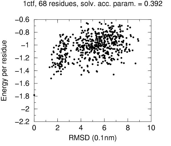
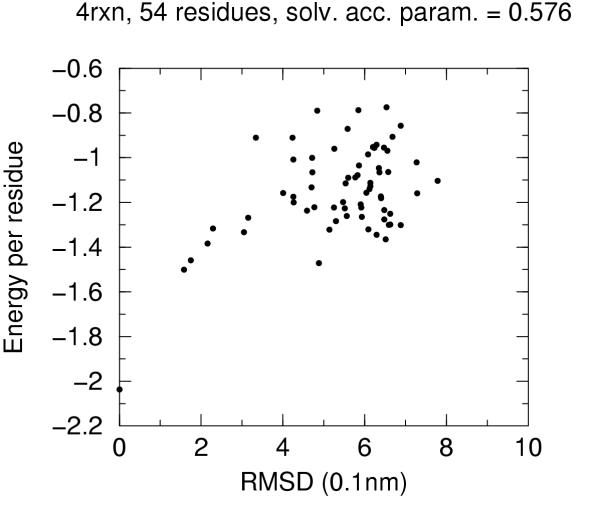
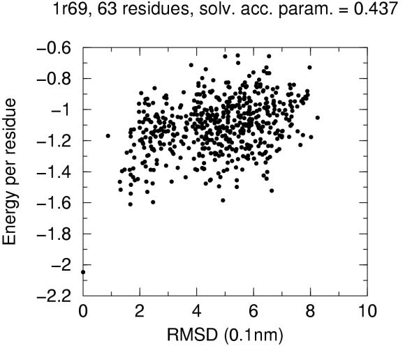
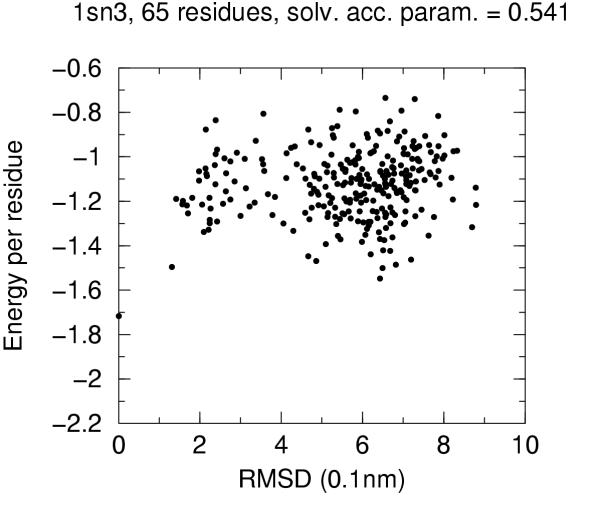
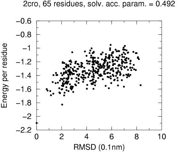
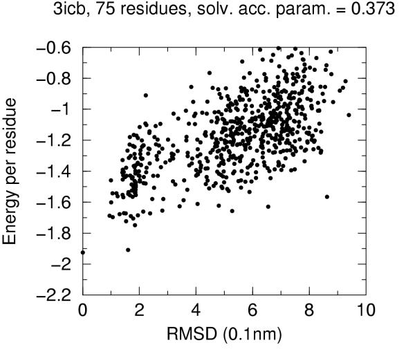
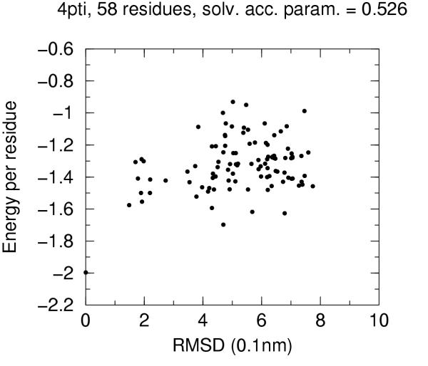
The solvent accessibility parameters on these decoys does not allow by itself discrimination of native conformation. Figures 4 to 10 report for each target protein of the set the contact energy per residue versus the RMSD with respect to the native structure. In view of the short length of the chains we chose a rather permissive 0.6 cutoff for the solvent accessibility parameter. Even with such a tolerant filter almost half of the decoys are discarded. For all proteins the native structure is well separated from the decoys. For some, but not for all, of the proteins (namely 2cro and 3icb) a correlation between contact energy and RMSD is apparent from the plot. In all cases, however, among the five lowest energy decoys there is a native-like structure with RMSD lower than 2.0 Å. These results should be compared with the results obtained both with similar approaches and with more refined methods like hybrid molecular mechanics – implicit solvent methods [26,31,29]. The performance of several energy functions tested on an enlarged version of the 4state decoys' set has been afforded by Park and Levitt [5]. It is apparent that the contact definition proposed in the present work has superior capabilities with respect to most similar approaches tested in that study. This is not just depending on cutoff choice for contact definition, because both rank score and z-score for native structure are consistently 1 and ranging between ca. 3.0 and ca. 6.0, respectively, for all cutoff choices, whereas the corresponding z-scores with contact potentials was between ca. 0.5 and ca. 3.0 on the enlarged set of decoys. On the other hand, when we compare our results (Figures 4 to 10) with the corresponding results obtained using the screened Coulomb potential-implicit solvent model (SCP-ISM) [26] or MM/PBSA free energy [31] we notice that with more refined methods a correlation between energy and RMSD from native structure is found which is much less pronounced with contact potentials.

Figure 4.

Energy vs. RMSD for 1ctf 4state decoys The contact energy is plotted against the RMSD from native structure for native structure and all decoy structures with solvent accesibility parameter lower than 0.6 (see text).

Figure 10.

Energy vs. RMSD for 4rxn 4state decoys The contact energy is plotted against the RMSD from native structure for native structure and all decoy structures with solvent accesibility parameter lower than 0.6 (see text).

Figure 5.

Energy vs. RMSD for 1r69 4state decoys The contact energy is plotted against the RMSD from native structure for native structure and all decoy structures with solvent accesibility parameter lower than 0.6 (see text).

Figure 6.

Energy vs. RMSD for 1sn3 4state decoys The contact energy is plotted against the RMSD from native structure for native structure and all decoy structures with solvent accesibility parameter lower than 0.6 (see text).

Figure 7.

Energy vs. RMSD for 2cro 4state decoys The contact energy is plotted against the RMSD from native structure for native structure and all decoy structures with solvent accesibility parameter lower than 0.6 (see text).

Figure 8.

Energy vs. RMSD for 3icb 4state decoys The contact energy is plotted against the RMSD from native structure for native structure and all decoy structures with solvent accesibility parameter lower than 0.6 (see text).

Figure 9.

Energy vs. RMSD for 4pti 4state decoys The contact energy is plotted against the RMSD from native structure for native structure and all decoy structures with solvent accesibility parameter lower than 0.6 (see text).

Evaluation of CASP4 predictive models

In order to test the chosen contact definition on a more realistic fold recognition scenario we tested all accepted predictive models including sidechains atoms accepted in the CASP4 experiment and for which the corresponding experimental structure has been solved and a link to the pdb file could be found on the CASP4 homepage http://predictioncenter.llnl.gov/casp4/. The range of legths, multimeric state and structural features of CASP4 targets is much wider than that of decoys [32]. Also the range of techniques used to generate the models is very wide in methods and quality (see e. g. abstracts available at http://predictioncenter.llnl.gov/casp4/). In such an experiment it is likely to be able to obtain either from own programs or from prediction servers a number of models and to be in the position of having to choose the best model or models for further study. One obvious difference with decoys' set tests is that it is not obvious that any native-like structure will be present in the ensemble of structures considered. This is indeed the case for many of the targets and models considered here.

Therefore, rather than looking for native fold discrimination, here we are interested in discriminating plausible (possibly native-like) structures from grossly misfolded ones.

In order to evaluate results and simulate a real prediction task we retained the ten lowest energy predictions which had an accessibility parameter lower than 0.486, a value chosen, for medium sized proteins, as a reasonable cutoff for applicability of the methodology. In a real prediction task, the ten lowest energy predictive models would be candidates for evaluation with more refined fold recognition methods. The results obtained in this test are summarized in Table 4. A prerequisite of the methodology is obviously that the native structure should be discriminated against all misfold predictive models. This is indeed the case for 30 out of 35 targets. The exceptions concerns: i) two out of the four NMR structures (targets 97 and 105, a putative Chaperone in dimeric form, and the SAND domain of a DNA binding protein, respectively); ii) the secreted frizzled protein 3 from mouse (target 106) which presents however a rather large solvent accessibility parameter (0.581) possibly due to its multimeric state; iii) porcine lactoglobulin (target 123) for which low RMSD predictions have lower contact energy possibly due to a domain swap in the dimerization domain; iv) phospholipase C beta from turkey (target 124) which presents unusually long helices (more than 80 residues). One of the lowest energy predictions, however, has also very long helices.

Table 4.

Summary of the results on the CASP4 accepted prediction models

target	pdb id.	n. res.	energy	s. a. par.	n. models	RMSD range	RMSD pred.	energy pred.	s. a. par. pred.
86	1fw9	164	-2.46	0.278	53	13.04 – 33.26	15.79	-1.77	0.48
87	1i74	304	-2.37	0.276	61	14.71 – 49.16	16.00	-1.61	0.46
89	1e4f	378	-2.44	0.266	70	13.98 – 67.53	13.98	-1.78	0.41
90	1g0s	201	-1.84	0.530	88	4.67 – 45.25	6.12	-1.51	0.46
92	1im8	219	-2.44	0.336	84	2.92 – 32.47	2.92	-1.77	0.46
94	1fsi	179	-2.23	0.443	56	9.78 – 38.71	15.24	-1.81	0.46
95	1l7c	234	-2.09	0.384	81	9.73 – 34.10	12.86	-1.94	0.42
96	1e2x	223	-2.41	0.328	82	3.18 – 31.22	3.65	-1.60	0.46
97	1g7d	106	-1.53	0.345	136	7.92 – 18.12	9.22	-1.59	0.45
98	1fc3	119	-2.45	0.461	115	7.50 – 40.42	11.36	-2.39	0.45
100	1qjv	342	-2.24	0.294	48	10.34 – 112.23	10.39	-1.48	0.48
102	1e68	70	-2.42	0.468	111	3.55 – 34.62	3.91	-0.60	0.46
103	1ga6	369	-2.64	0.217	67	4.38 – 71.71	4.38	-2.04	0.38
104	1fl9	157	-2.22	0.421	88	6.21 – 37.95	7.95	-1.70	0.47
105	1h5p	95	-1.29	0.462	91	6.10 – 24.11	11.99	-1.38	0.40
106	1ijx	125	-2.39	0.581	75	8.47 – 26.55	9.21	-2.76	0.48
107	1i82	189	-2.22	0.273	88	10.88 – 38.55	12.75	-1.68	0.45
108	1j83	178	-2.34	0.276	64	7.75 – 66.56	7.76	-1.54	0.47
111	1e9i	430	-2.30	0.200	92	1.60 – 81.08	1.86	-1.92	0.23
112	1e3j	350	-2.65	0.269	87	11.21 – 97.16	11.93	-2.02	0.36
113	1e3w	251	-2.27	0.342	92	2.03 – 41.72	2.40	-2.02	0.35
114	1gh5	87	-2.55	0.457	85	6.58 – 32.14	6.58	-0.58	0.37
115	1fwk	296	-2.47	0.280	56	12.16 – 59.64	18.68	-1.40	0.46
116	1ewq	746	-2.28	0.315	40	8.38 – 115.82	14.41	-1.50	0.47
117	1j90	195	-2.20	0.362	79	2.87 – 35.27	2.87	-1.68	0.38
118	1fzr	129	-1.53	0.681	80	13.72 – 26.35	18.82	-1.33	0.46
119	1krh	337	-2.50	0.309	87	2.74 – 82.93	2.88	-2.06	0.34
120	1fu1	174	-1.72	0.563	50	1.32 – 44.20	19.04	-1.15	0.31
121	1g29	372	-2.50	0.329	90	3.35 – 100.88	3.70	-1.90	0.38
122	1geq	241	-2.65	0.274	97	2.09 – 41.36	2.73	-2.08	0.39
123	1exs	160	-2.11	0.481	111	3.30 – 36.92	3.42	-2.17	0.35
124	1jad	235	-1.22	0.435	64	3.51 – 89.91	23.85	-1.25	0.47
125	1gak	137	-1.93	0.378	113	3.26 – 31.68	3.26	-1.75	0.41
126	1f35	157	-1.99	0.487	81	9.70 – 29.48	13.96	-1.23	0.47
127	1g8p	321	-2.38	0.327	74	11.15 – 67.04	17.29	-1.98	0.43

Results obtained with contact definition SC+CA with a 1.0 Å cutoff on targets in the CASP4 experiment are summarized. Columns list the target number, the corresponding pdb code, the number of residues, the energy per residue of the experimental structure, the solvent accessibility parameter of the experimental structure, the number of models considered, the range of RMSD, the RMSD of the best structural prediction among the ten lowest energy models, the energy per residue for the same structure and its solvent accessibility parameter.

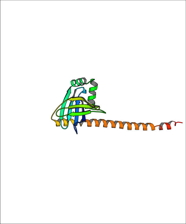
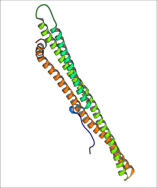
Problems with NMR structures versus X-ray structures have been repeatedly pointed out (see e. g. ref. [31]) so that failure in native structure recognition could also be due to artifacts in structure generation from NMR restraints. These few examples point out the complexity of predicting real proteins, where biological insight and additional informations about the function, the environment, ligands and multimeric state is of utmost importance. It should be noticed that only 15 targets had predictions (in the selection we did) with RMSD lower than 5 Å. For 12 out of these 15 targets a low RMSD prediction (less than 5 Å) was found among the ten lowest energy predictive models. For one of the remaining three targets (target 90) the chosen prediction has still rather low RMSD (6.125 Å). The other two targets (targets 120 and 124) where the method fails to recognize low RMSD predictions are dimers where only a monomer or part of it are modelled. For the sake of clarity the structure of the chains to be predicted (pdb id. 1fu1 and 1jad, respectively) are reported in Figures 11 and 12. Overall these results demonstrate the capability of contact energy (corresponding to the optimal contact definition) to recognize low RMSD predictions among the lowest energy models, provided that the structure to be modelled has the typical features of soluble globular proteins. The same results however point out that it is difficult to assess the reliability of the predictive models, because there is almost no correlation between the energy per residue and the proximity of the models to the native structure (when all pairs RMSD-energy are pooled together), at least for the models we selected from the CASP4 experiment.

Figure 11.

Structure of target 120 in the CASP4 experiment The structure of the N-terminal domain of human DNA repair protein XRCC4 is shown (pdb id. 1fu1, chain A). The long helix is in contact with another chain in the pdb file.

Figure 12.

Structure of target 124 in the CASP4 experiment The structure of the C-terminal domain of turkey phospolipase C beta is shown (pdb id. 1jad, chain A). The long helix forms a coiled coil with the other chain in the pdb file.

Conclusions

The fold prediction problem can be divided in two parts: the generation of alternative conformations and the estimation of the stability of every available structure. The second task is usually accomplished using structural information available from the protein data bank. Based on the theory of the potential of mean force, empirical contact energies for any pair of amino acids have been derived. Crucial to this derivation and its performance in fold recognition, are: i) the definition of contact and ii) the definition of applicability limits.

The analysis presented in this work shows that the best definition of contact is the one involving the minimum distance between van der Waals spheres of any two side chain or alpha carbon atoms belonging to the two amino acids, and employing a cutoff distance around 1.0 Å. The performance of the proposed definition on decoys' sets is superior to other proposed contact definitions, as far as native structure recognition is concerned. An ad hoc defined solvent accessibility parameter helps in discriminating against structures not conforming to model assumptions.

Indeed, contact energies refer to a desolvation process and therefore crucially depend on the solvent. Proteins that do not show a "normal" solvent accessibility most likely do not conform to model assumptions and have been indeed found, by later inspection, to be associated in macromolecular complexes or to be membrane proteins.

A more intriguing issue is understanding why the approach fails on short monomeric chains. A possible explanation is that entropic restrictions on backbone atoms ensuing from folding are on average different for short chains and for larger chains from which the energy contact table is mainly derived.

Results obtained in a real prediction scenario, like the one set up by the CASP experiment, are twofold: first, a gross screening (discarding approximately nine tenths of the predictive models) can be afforded by evaluating the solvent accessibility parameter and comparing the contact energy among models; second, the correlation between the energy per residue of a model and its similarity to native structure, if there is any, is very poor, and therefore the reliability of the best predictive models, for each target, cannot be assessed and more refined methods, like hybrid molecular mechanics – implicit solvent methods should be used in later stages of the prediction procedure.

Materials and methods

We discuss in the following sections the theoretical framework, based on the potential of mean force theory [33], which allows to define empirical contact energies from observed statistical contact preferences [34]. This approach received several objections. One of the most serious concerns the additivity of contact energies [18]. The general possibility of dissecting a free energy (e. g. of folding or binding) into components faces several problems which have been clearly pointed out by Mark and van Gunsteren [19]. One clear proof that these issues are well-founded is that folding energies obtained from contact energies are usually one order of magnitude larger than expected. Notwithstanding all these problems contact energies and free energy decomposition appear still successful in many instances.

Potential of mean force and empirical contact energies

We consider a system composed by many interacting bodies, which will be ultimately amino acids. The probability that a system composed by N particles is in the state described by coordinates is given by:

where U is the potential energy of the system, k is Boltzmann constant and T is the temperature. Let us assume that bodies 1 and 2 belong to different body types i and j, which are represented by N_i and N_j bodies, respectively. Then, the probability, which we assume to depend only on the distance r, that a body of type i is at a distance r from a body of type j, independently of all other particles' positions, is:

In the absence of any interaction among the bodies the probability depends only on their density:

dP_ij0 = ρ_i0ρ_j0Vdr

where V is the volume, and are the densities of bodies of type i and j, respectively. The ratio between the actual and reference probability density is the distribution function g_ij(r):

dP_ij(r) = ρ_i0ρj0g_ij(r)drV

which may be written in a form similar to a Boltzmann distribution according to the potential of mean force w_ij(r):

Conversely the potential of mean force may be expressed as follows:

w_ij(r) = -kT ln g_ij(r)

The equation above allows one to derive the potential of mean force from the observed distribution function over a representative ensemble of configurations. The derivative of the potential of mean force gives the mean force, averaged over all other degrees of freedom, between bodies i and j, as can be shown taking the derivative of the equation above.

In order to treat all interactions among amino acids in terms of contacts we should schematize continuously varying potential of mean force functions as step functions assuming a value different from zero only in the distance range corresponding to a contact. In order to make this approximation in a consistent way we will introduce in the next section the Bethe approximation.

Bethe approximation

The potential of mean force described above may be schematised by a well function. For distances shorter than the width of the well the two bodies interact and they are said to be in contact. This is partly justified by the short-range nature of most important interaction forces among amino acids. The correspondence between actual and schematised potential of mean force is depicted in Figure 13.

Figure 13.

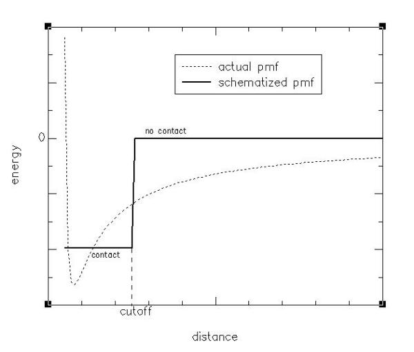
Contact definition representation A schematic diagram relating contact definition to the potential of mean force is shown.

In order to define properly the depth of the well function, once a contact distance (r_cutoff) has been chosen, it is worth to consider the contact probability

where r is a scalar expressing, for a fixed body, the distance with any other body.

Introducing the well potential f, which is constant and equal to W for every r between the core and cutoff radius, the contact probability P_c can be expressed as:

It should be noted that the term ρ₀ΔV represents the contact probability P_0c in the case of no interactions other than the repulsive ones. The equation above allows one to calculate the well depth W from the observed contact probability and from the reference contact probability :

It is worth noting that the two factors affecting the reference contact probability are ρ i.e. the density of the particle considered, and ΔV i. e. the volume available for a contact. This reference state implies that the expected number of contacts, in the absence of interactions between amino acids, will be proportional to the amino acid type density, i.e. their number, and the volume where a contact is defined, i. e. the number of possible contacts, which is often named the coordination number. A special kind of residue must be associated to solvent, to describe it in a way which is consistent with this framework, as we discuss later. The above equations relate the observed contact probability with the corresponding contact energy. In order to measure contact probabilities we must sample the most probable conformations of an ensemble of amino acids (e. g. constituting a protein chain) in an efficient way. An ad hoc way to treat this problem is described in the next section.

Conformational space sampling

To calculate the potential of mean force, sampling of the conformational space is necessary for every protein, but this operation is not possible because we only have the native conformation for each polypeptide chain. Every protein structure is considered to be a particular configuration, more precisely the most probable one, of a system of interacting amino acids and solvent. The probability of a contact between amino acids of different types will be defined based on the number of observed contacts in native conformations. This in turn requires a definition of contact.

Definition of a contact

A contact is defined to exist only if the distance between residues is less than a cutoff value. The distance between residues is usually defined as the minimum distance between parts of an amino acid.

Simple distance definitions based on alpha or beta carbon positions do not take into account differences in amino acid shape and volume. The choice of all heavy atoms including hydrogen-bond forming backbone atoms, on the other hand, tends to mask amino acid contact specificity under non-specific backbone contacts. As will be shown, best results are obtained considering only heavy atoms of side chains and alpha carbons.

An important approximation is neglect of the effect of chain connectivity. Obviously contacts between residues that are neighbours in sequence are much more frequently observed than contacts between residues separated by a long stretch of chain. The only correction here introduced that takes into account chain connectivity is ignoring contacts between residues that are next to each other in the sequence: because of the peptide bond, those contacts cannot but exist. An implicit assumption in this scheme is that contacts between residues close in sequence show the same preferences as residues widely separated. The matrix of contacts, whose element i, j is 1 if there is a contact between residues i and j, and 0 otherwise, is a very compact way to represent a protein structure independently from a reference system. Chirality information, which is not present in the matrix, is enforced by amino acids chirality itself. In the following sections, we will examine how to treat contacts with solvent whose definition is not so straightforward.

Contacts with the solvent

Contacts with solvent molecules, often not available in the PDB files, must be estimated indirectly. The number of contacts established by each amino acid depends on the nature and relative orientation of the contacting residues. In order to get rid of the solvent contacts problem, the coordination number has been estimated for non solvent accessible residues as their number of contacts. The dependence on contacts specificity has been neglected and average values have been used. In practice the number of contacts, for different contact definitions, has been plotted versus accessibility (computed using a routine of the WHATIF program [35]) for each amino acid type. The intercept of the regression curve at zero accessibility was then defined as the coordination number. This procedure increases statistical significance for all preferentially solvent exposed residues, compared to just examining buried residues. The coordination number represents the average number of contacts made by a buried residue.

Similar to a lattice model, the coordination number establishes the number of contacts made by every residue at any time, either with other residues or solvent (Table 5).

Table 5.

Amino acid coordination numbers and solvent accesibilities

Residue	coord. n.	am (Å2)	σa (Å2)
CYS	7	6.683	10.044
MET	8	13.818	15.638
PHE	9	12.747	14.597
ILE	8	9.487	13.742
LEU	8	10.454	12.840
VAL	7	8.523	10.375
TRP	10	15.233	16.309
TYR	9	16.430	14.349
ALA	5	9.865	10.059
GLY	4	8.675	7.659
THR	6	14.775	10.542
SER	5	13.687	9.927
ASN	7	19.319	12.195
GLN	7	22.667	13.855
GLU	7	23.294	12.322
ASP	6	17.791	10.786
HIS	8	19.122	14.963
ARG	9	31.045	17.145
LYS	8	33.329	13.796
PRO	6	17.674	12.097

Coordination numbers with contact definition SC+CA with a 1.0 Å cutoff and solvent accessibility values. a_m is the mean accessibility and σ_a is the accessibility's standard deviation estimated for each amino acid type. a_m and σ_a values have been obtained from the file EVAACC.ACC from program WHATIF.

Because interactions among amino acids are estimated using the concept of contact, we need an analogous method to express the interactions with the solvent: in this context, the concept of residue-equivalent of solvent is defined.

We assume that the difference between the coordination number and actual number of contacts is due to contacts with solvent-equivalent residues. Therefore the coordination number of solvent-equivalent residue is the weighted mean of the coordination numbers of amino acid residues.

Reference state

In order to compute the contact energy the expected number of contacts, assuming no preferential contacts, must be computed. Consistent with the previous discussion, the reference state is calculated considering both residue representativeness and coordination number. Similar to a lattice model, the probability that a chosen contact involves amino acid types i and j is:

p_ijαN_iN_icN_jN_jc + N_jN_jcN_iN_ic = 2N_iN_icN_jN_jc when i ≠ j

p_iiαN_iN_icN_iN_ic

where N_i is the number of amino acids of type i and N_ic is the coordination number of amino acid of type i. The probability's summation over i and j must be 1:

where k is a proportionality constant. When we introduce the total number of contacts N_c we have:

and constant k can be estimated by:

Therefore the number of contacts in the reference state can be estimated by the following expressions:

The number of observed and expected contacts for each amino acid type and solvent-equivalent residue has been computed for each protein and summed over all proteins, thus obtaining the number of total expected and observed contacts:

where the superscript p indicates each protein of the dataset, which must be suitably chosen.

Selection of proteins for the construction of the dataset

Each protein is described as a collection of 20 different amino acid's types, and the entire remaining space is assumed to be aqueous solvent. Other groups, like polysaccharides, lipids, nucleic acids and prosthetic groups, are ignored. In this context, all non soluble proteins and proteins interacting with other groups cannot be adequately described by the model. We assume that these proteins can be discriminated because we expect atypical solvent exposure properties, like e.g. the presence of large exposed areas of hydrophobic residues for membrane proteins which are actually exposed to a lipid environment.

For every amino acid type, typical solvent exposure is expressed in terms of mean and standard deviation of observed accessibility distribution, and is provided by the internal database of the program Whatif [35].

For a given test protein, a solvent accessibility parameter is introduced that takes into account residue accessibilities larger than the corresponding typical value:

where: a(i) is the accessibility observed for residue i, a_m(i) is the mean accessibility estimated for the i^th residue's amino acidic type, σ_a(i) is the accessibility's standard deviation estimated for the i^th residue's amino acidic type, N is the number of amino acids and δ is the Heaviside function.

The rationale behind this choice is that, due to the possible neglect of other molecules or groups not explicitly represented, the calculated accessibility can only overestimate the real accessibility.

In order to perform proper statistical analysis, it is necessary to avoid database information redundancy: similar to other works conducted on protein structures, only proteins belonging to the list called pdb_select 25% [36,37], released in October 2000, were considered. Moreover, only protein's structures resolved by X-ray crystallography were accepted here, and non-complete coordinate sets, or sets containing non-standard aminoacids, were rejected. The remaining 746 chains were ranked according to the solvent accessibility parameter, and only the arbitrary number of 500 best structures were retained, which formed our proteins' dataset. In this way, proteins with solvent accessibility parameter greater than 0.486 were rejected.

Empirical contact energies

Provided with energies for residue-residue, residue-solvent and solvent-solvent contacts, we consider the folding reaction starting from a completely hydrated conformation. For each contact established in the native structure the considered reaction is

i0 + j0 → ij + 00

where i, j and 0 indicate residues of type i, j and solvent, respectively.

A strong assumption is made here, and in similar works, that the free energy corresponding to products and reactants may be simply computed by adding contact potential of mean force for each contact in the products and the reactants.

Thus the corresponding free energy can be calculated by the following formula:

where: t_ij is the ratio of the number of contacts observed and the number of contacts in the reference state. Finally, the energy of folding starting from a completely solvated conformation is:

where i and j run on all aminoacid type. In this reaction every amino acid contact replaces a contact with solvent and therefore the number of newly formed contacts between solvent-equivalent residues is equal to the number of contacts between amino acidic residues.

Alternative conformations

In order to test empirical energies for fold recognition, alternative conformations must be compared and the native conformation must be assigned a lower energy than alternative conformations. Chosen a test protein, alternative conformations can be obtained essentially in two ways: modelling the sequence to structures available from a structural database, or producing different possible and physically admissible conformations by means of computational methods.

As a cheap approximation to threading procedure and for a quick test of the quality of the empirical contact energies derived from different contact definitions, we assumed that each sequence (truncated if necessary) in the protein dataset could assume a conformation corresponding to the contact matrix (or sub-matrix) of any other protein in the dataset itself. In this procedure amino acids do not maintain their coordination numbers, i.e. a small residue may be assigned a large number of contacts and viceversa. Although more clever threading procedures exist, we used this as a gross test, reasoning that in this non optimal nor refined superposition, the native contact matrix must have a much lower energy than any other contact matrix. Thus good discrimination in this gross test is a preliminary minimal requirement for any empirical contact energy table.

Contrary to this procedure, when alternative contact maps are derived from alternative structures, for a given protein chain, produced by computational methods, the sequence – contact matrix superposition will be always properly performed. In these more accurate tests, alternative conformations have been referred to as decoys. The sets of decoys employed here are freely available from the URL http://dd.stanford.edu. Here, we used four different sets of decoys, which are called misfold [25], 4state_reduced [5], lmds [Kesar and Levitt, unpublished] and fisa_casp3 [38]. In the following, the first and last sets, respectively, will be simply referred to as 4state and casp3.

The misfold set contains a single decoy for 26 chains obtained by gapless threading of the sequence onto another structure. Side chains have been placed using a Monte Carlo annealing procedure in rotamer space using an atom-atom simple potential. Native and decoy structures may have radically different secondary structures, which may conflict with local propensities.

The 4state decoy set includes ca. 650 decoys for each of seven small proteins. The decoys have been generated imposing to each residue one out of four allowed conformations. For ten ("hinge") residues all conformations have been generated, for all other residues the best one fitting to local structure have been used. The very large set thus obtained has been filtered using steric and compactness criteria and the best scoring decoys (using a variety of scoring functions) have been retained. These decoys retain local secondary structures, have compactness typical of native proteins and contain a large number of decoys with low RMSD from native structure.

The local minima decoy set (lmds) includes ca. 450 alternative conformations for each of 11 proteins. This set has been generated randomizing the torsional angles of loop regions and by minimization in torsion angle space using an energy function which entails atom-atom interactions and additional terms that promote compactness and formation of secondary structure. In most cases native structure could be distinguished from decoys using the solvent accessibility parameter.

The casp3 decoy set includes ca. 1400 decoys for each of 4 proteins generated by ab initio fragment assembly using fragments with similar local sequences. Most of the models have solvent accessibility parameter values higher than native structure.

The detailed description of all these decoys and additional references are available from the URL: http://dd.stanford.edu

Evaluation of discrimination power

The energy distribution assigned to different alternative conformations is analysed through two different parameters, subsequently described.

For a given sequence, alternative contact matrices are ranked according to the corresponding energies. The rank score is the rank position of the native matrix. Thus if the energy corresponding to the native matrix is the lowest one, the rank score assumes value 1.

A good fold recognition system is able not only to discriminate the native conformation, assigning to it the lowest energy, but also to separate it in a clearcut way from other non-native conformations. The energy distribution is characterised by a mean and a standard deviation, which are used to estimate the extent of such a separation. The z-score is defined (a minus sign is introduced here, compared to standard definitions) as the distance of the energy of the native conformation from the average energy measured in standard deviation units:

The more positive is the value of the z-score, the greater is the separation of the native conformation from the alternative ones.

The z-score has been used in recent years to derive and assess the quality of potentials for protein folding (see e.g. [39-41]).

References

- Mirny L, Shakhnovich E. Protein folding theory: from lattice to all-atom models. Ann Rev Biophys Biomol Struct. 2001;30:361–396. doi: 10.1146/annurev.biophys.30.1.361. [DOI] [PubMed] [Google Scholar]
- Bonneau R, Baker D. Ab initio protein structure prediction: progress and prospects. Ann Rev Biophys Biomol Struct. 2001;30:173–89. doi: 10.1146/annurev.biophys.30.1.173. [DOI] [PubMed] [Google Scholar]
- Anfinsen CB. Principles that govern the folding of protein chains. Science. 1973;181:223–230. doi: 10.1126/science.181.4096.223. [DOI] [PubMed] [Google Scholar]
- Sippl MJ. Knowledge-based potentials for proteins. Curr Opin Struct Biol. 1995;5:229–35. doi: 10.1016/0959-440X(95)80081-6. [DOI] [PubMed] [Google Scholar]
- Park B, Levitt M. Energy function that discriminate x-ray and near-native folds from well-constructed decoys. J Mol Biol. 1996;258:367–392. doi: 10.1006/jmbi.1996.0256. [DOI] [PubMed] [Google Scholar]
- Vendruscolo M, Kussell E, Domany E. Recovery of protein structure from contact maps. Fold Des. 1997;2:295–306. doi: 10.1016/S1359-0278(97)00041-2. [DOI] [PubMed] [Google Scholar]
- Tanaka S, Scheraga HA. Medium- and long-range interaction parameters between amino acids for predicting three-dimensional structures of proteins. Macromolecules. 1976;9:945–50. doi: 10.1021/ma60054a013. [DOI] [PubMed] [Google Scholar]
- Miyazawa S, Jernigan RL. Estimation of effective interresidue contact energies from protein crystal structures: quasi-chemical approximation. Macromolecules. 1985;18:534–552. [Google Scholar]
- Miyazawa S, Jernigan RL. Residue-residue potentials with a favorable contact pair term and an unfavorable high packing density term, for simulation and threading. J Mol Biol. 1996;256:623–644. doi: 10.1006/jmbi.1996.0114. [DOI] [PubMed] [Google Scholar]
- Miyazawa S, Jernigan RL. Self-consistent estimation of inter-residue protein contact energies based on an equilibrium mixture approximation of residues. Proteins. 1999;34:49–68. doi: 10.1002/(SICI)1097-0134(19990101)34:1<49::AID-PROT5>3.3.CO;2-C. [DOI] [PubMed] [Google Scholar]
- Miyazawa S, Jernigan RL. An empirical energy potential with a reference state for protein fold and sequence recognition. Proteins. 1999;36:357–69. doi: 10.1002/(SICI)1097-0134(19990815)36:3<357::AID-PROT10>3.3.CO;2-L. [DOI] [PubMed] [Google Scholar]
- Vendruscolo M, Domany E. Efficient dynamics in the space of contact map. Fold Des. 1998;3:329–336. doi: 10.1016/S1359-0278(98)00045-5. [DOI] [PubMed] [Google Scholar]
- Vendruscolo M, Domany E. Protein folding using contact maps. Vitam Horm. 2000;58:171–212. doi: 10.1016/s0083-6729(00)58025-x. [DOI] [PubMed] [Google Scholar]
- Zhang C, Vasmatzis G, Cornette JL, DeLisi C. Determination of atomic desolvation energies from the strucures of crystallized proteins. J Mol Biol. 1997;267:707–726. doi: 10.1006/jmbi.1996.0859. [DOI] [PubMed] [Google Scholar]
- Skolnick J, Jaroszewski L, Kolinski A, Godzik A. Derivation and testing of pair potentials for protein folding. when is the quasichemical approximation correct? Prot Sci. 1997;6:676–688. doi: 10.1002/pro.5560060317. [DOI] [PMC free article] [PubMed] [Google Scholar]
- Samudrala R, Moult J. An all-atom distance-dependent conditional probability discriminatory function for protein structure prediction. J Mol Biol. 1998;275:895–916. doi: 10.1006/jmbi.1997.1479. [DOI] [PubMed] [Google Scholar]
- Zhang C, Kim S. Environment-dependent residue contact energies for proteins. Proc Natl Acad Sci. 2555;97:2550–2000. doi: 10.1073/pnas.040573597. [DOI] [PMC free article] [PubMed] [Google Scholar]
- Ben-Naim A. Statistical potentials extracted from protein structures: Are these meaningful potentials? J Chem Phys. 3706;107:3698–1997. doi: 10.1063/1.474725. [DOI] [Google Scholar]
- Mark AE, van Gunsteren WF. Decomposition of the free energy of a system in terms of specific interactions. implications for theoretical and experimental studies. J Mol Biol. 1994;240:167–176. doi: 10.1006/jmbi.1994.1430. [DOI] [PubMed] [Google Scholar]
- Vendruscolo M, Najmanovich R, Domany E. Can a pairwise contact potential stabilize native protein folds against decoys obtained by threading? Proteins. 2000;38:134–148. doi: 10.1002/(SICI)1097-0134(20000201)38:2<134::AID-PROT3>3.0.CO;2-A. [DOI] [PubMed] [Google Scholar]
- Fariselli P, Casadio R. Prediction of the number of residue contacts in proteins. Proc Int Conf Intell Syst Mol Biol. 2000;8:146–51. [PubMed] [Google Scholar]
- Fariselli P, Olmea O, Valencia A, Casadio R. Progress in predicting inter-residue contacts of proteins with neural networks and correlated mutations. Proteins. 2001;5:157–62. doi: 10.1002/prot.1173. [DOI] [PubMed] [Google Scholar]
- Moult J, Hubbard T, Fidelis K, Pedersen J. Critical assessment of methods of protein structure prediction (casp): Round iii. Proteins. 1999;3:2–6. doi: 10.1002/(SICI)1097-0134(1999)37:3+<2::AID-PROT2>3.3.CO;2-U. [DOI] [PubMed] [Google Scholar]
- Berman HM, Westbrook J, Feng Z, Gilliland G, Bhat TN, Weissig H, Shindyalov IN, Bourne PE. The protein data bank. Nucl Acids Res. 2000;28:235–242. doi: 10.1093/nar/28.1.235. [DOI] [PMC free article] [PubMed] [Google Scholar]
- Holm L, Sander C. Evaluation of protein models by atomic solvation preference. J Mol Biol. 1992;225:93–105. doi: 10.1016/0022-2836(92)91028-n. [DOI] [PubMed] [Google Scholar]
- Hassan SA, Mehler EL. A critical analysis of continuum electrostatics: the screened coulomb potential – implicit solvent model and the study of the alanine dipeptide and discrimination of misfolded structures of proteins. Proteins. 2002;47:45–61. doi: 10.1002/prot.10059.abs. [DOI] [PubMed] [Google Scholar]
- Petrey D, Honig B. Free energy determinants of tertiary structure and the evaluation of protein models. Protein Sci. 2191;9:2181–2000. doi: 10.1110/ps.9.11.2181. [DOI] [PMC free article] [PubMed] [Google Scholar]
- Lazaridis T, Karplus M. Discrimination of the native from misfolded protein models with an energy function including implicit solvation. J Mol Biol. 1999;288:477–87. doi: 10.1006/jmbi.1999.2685. [DOI] [PubMed] [Google Scholar]
- Felts AK, Gallicchio E, Wallqvist A, Levy RM. Distinguishing native conformations of proteins from decoys with an effective free energy estimator based on the opls all-atom force field and the surface generalized born solvent model. Proteins. 2002;48:404–22. doi: 10.1002/prot.10171. [DOI] [PubMed] [Google Scholar]
- Rhee S, Martin RG, Rosner JL, Davies DR. A novel dna-binding motif in mara: the first structure for an arac family transcriptional activator. Proc Natl Acad Sci USA. 0418;95:10413–1. doi: 10.1073/pnas.95.18.10413. [DOI] [PMC free article] [PubMed] [Google Scholar]
- Lee MR, Kollman PA. Free-energy calculations highlight differences in accuracy between x-ray and nmr structures and add value to protein structure prediction. Structure. 2001;9:905–16. doi: 10.1016/S0969-2126(01)00660-8. [DOI] [PubMed] [Google Scholar]
- Murzin A, Hubbard T. Prediction targets of casp4. Proteins Suppl. 2001;5:8–12. doi: 10.1002/prot.10055. [DOI] [PubMed] [Google Scholar]
- Hill T. An introduction to statistical mechanics. Dover Publications. 1956.
- Sippl MJ. An approch to the knowlodge-based prediction of local structures in globular proteins. J Mol Biol. 1990;213:859–883. doi: 10.1016/s0022-2836(05)80269-4. [DOI] [PubMed] [Google Scholar]
- Vriend G. What if: A molecular modeling and drug design program. J Mol Graph. 1990;8:52–54. doi: 10.1016/0263-7855(90)80070-V. [DOI] [PubMed] [Google Scholar]
- Hobohm U, Scharf M, Schneider R, Sander C. Selection of representative protein data sets. Prot Sci. 1992;1:409–417. doi: 10.1002/pro.5560010313. [DOI] [PMC free article] [PubMed] [Google Scholar]
- Hobohm U, Sander C. Enlarged representative set of protein structures. Prot Sci. 1994;3:522–524. doi: 10.1002/pro.5560030317. [DOI] [PMC free article] [PubMed] [Google Scholar]
- Simons KT, Kooperberg C, Huang E, Baker D. Assembly of protein tertiary structures from fragment with similar local sequences using simulated annealing and bayesian scoring function. J Mol Biol. 1997;268:209–225. doi: 10.1006/jmbi.1997.0959. [DOI] [PubMed] [Google Scholar]
- Zhang L, Skolnick J. What should the z-score of native protein structures be? Protein Sci. 1207;7:1201–1998. doi: 10.1002/pro.5560070515. [DOI] [PMC free article] [PubMed] [Google Scholar]
- Vendruscolo M, Mirny LA, Shakhnovich EI, Domany E. Comparison of two optimization methods to derive energy parameters for protein folding: perceptron and z-score. Proteins. 2000;41:192–201. doi: 10.1002/1097-0134(20001101)41:2<192::AID-PROT40>3.3.CO;2-V. [DOI] [PubMed] [Google Scholar]
- Vendruscolo M. Assessment of the quality of energy functions for protein folding by using a criterion derived with the help of the nois go model. J Biol Phys. 2001;27:205–215. doi: 10.1023/A:1013152026788. [DOI] [PMC free article] [PubMed] [Google Scholar]