Testing for differentially expressed genes with microarray data

Abstract

This paper compares the type I error and power of the one- and two-sample t-tests, and the one- and two-sample permutation tests for detecting differences in gene expression between two microarray samples with replicates using Monte Carlo simulations. When data are generated from a normal distribution, type I errors and powers of the one-sample parametric t-test and one-sample permutation test are very close, as are the two-sample t-test and two-sample permutation test, provided that the number of replicates is adequate. When data are generated from a t-distribution, the permutation tests outperform the corresponding parametric tests if the number of replicates is at least five. For data from a two-color dye swap experiment, the one-sample test appears to perform better than the two-sample test since expression measurements for control and treatment samples from the same spot are correlated. For data from independent samples, such as the one-channel array or two-channel array experiment using reference design, the two-sample t-tests appear more powerful than the one-sample t-tests.

INTRODUCTION

Recent advances in cDNA microarray technology provide exciting tools for studying the expression levels of thousands of distinct genes simultaneously. There are two main platforms for cDNA microarray: nylon membrane-based filter arrays and chemically coated glass-based arrays. The nylon membrane arrays are hybridized with ³³P or ³⁵S-labeled cDNA targets, and glass arrays are hybridized with fluorescent dye-labeled targets. The nylon array is also used with the colorimetric detection (1). The simplest microarray experiment is to study changes in gene expression levels between a reference sample and a treated (toxin or drug) sample. In the experiment, samples of DNA clones with known sequence content are spotted and immobilized onto a glass slide or nylon filter. The mRNA extracted from the tissue cell under study is purified, reversed-transcribed into cDNA and labeled with radioactive markers or with green or red fluorescent dyes. Labeled cDNA hybridizes to the spots containing complementary sequences on the array. After hybridization, the radioactive or fluorescent signal intensities are measured using a phosphoimager or laser scanner, respectively. One intensity is measured on each spot for the radiation-labeled array (one-channel array) while two intensities are measured on each spot for the fluorescence dye-labeled array (two-channel array). In both cases, the intensities are surrogates for the expression levels of genes in the sample under study.

In a two-channel experiment, the same spot is used to assess the expression of a gene for the control sample and the treated sample labeled with red and green (or vice versa), respectively. The expression levels of the two samples can be compared for each gene in an array. The ratio of the fluor intensity for each spot measures the relative abundance of the corresponding gene under two different experimental conditions. In contrast, in a one-channel experiment, the expression levels of a gene for the control and treated samples are measured on two different arrays. The expression levels of the control and treatment arrays are compared to assess the difference between two samples.

It has been recognized that there are many sources of systematic variation, spatial heterogeneity and signal saturation, in assigning expression levels to the measured intensities. The expression levels from the two measurements are not directly comparable. Adjustments of the expression data should be performed prior to statistical analysis. Yang et al. (2) and Irizarry et al. (3) described several normalization methods for the two-channel and one-channel arrays, respectively.

A goal of the microarray analysis is to identify a subset of genes that are differentially expressed between the control and treated samples. Draghici (4) gave a review and comparison of currently proposed methods for detecting the set of differentially expressed genes. In general, a gene is said to be differentially expressed if the ratio in absolute value of the expression levels between the treated group to the control exceeds a certain threshold (5), e.g. 2- or 4-fold change. These genes are classified as altered genes. This approach is deficient in some respects. For example, the ratio at the lower levels can be more different than that at the higher levels. Furthermore, gene expression measurements in hybridization experiments are noisy; e.g. the coefficient of variation in gene expression in mouse liver was found to be >30% among 80% of genes tested and >50% of the 56% of genes (6). Alternatively, Newton et al. (7) proposed an improved method of inferring fold changes by deriving the posterior odds of change within a similar model. Furthermore, the statistical significance testing approach and ANOVA can also be applied to identify differentially expressed genes (8–10).

Standard statistical methods have been used for comparisons of intensity levels among treatments one gene at a time (11). The log-transformed normalized intensities from two groups can be compared using either the one-sample or two-sample t-test (8,9). These two approaches represent different underlying model assumptions. The two-sample t-test assumes the distribution of the log-transformed intensity data in each group is independently and identically normally distributed, while the one-sample t-test assumes that the paired distribution of treated and control groups is normally distributed. In this paper we compare these two different testing approaches and compare them to permutation tests for identifying differentially expressed genes with replicate arrays. All models and methods described here are not restricted to any specific microarray platform or technology.

MATERIALS AND METHODS

Statistical models for background-subtracted raw intensity data

Assume that the experimental design for two cDNA samples on the array are a control and a treatment sample, for example, the control sample is assigned to the green dye and the treated sample is assigned to the red dye. Because of different labeling efficiencies or different scanning sensitivities to the two dyes, the so-called dye swap design with two arrays is often used to account for dye biases. In the dye swap design, on array 1, the control sample is assigned to the green dye and the treated sample is assigned to the red dye; the dye assignments are reversed on array 2. We first present a model for gene expression data from this type of two-channel cDNA microarray design. We will consider the data from another type of two-channel cDNA microarray design and from a one-channel microarray.

It has been recognized that microarray spot intensity, in general, is approximately log-normally distributed with the standard deviation approximately proportional to the magnitude of intensity (mean), e.g. Black and Doerge (12), Chen et al. (13) and Ideker et al. (14). Furthermore, two intensity measurements of the same spot are correlated. A model for background-subtracted intensities (without a normalization) for a spot (gene) on the array is

X_ijc = µ_ice^ηijc + ε_ijc

X_ijt = µ_ite^ηijt + ε_ijt,

where (µ_ic,µ_it) represents the paired true expression levels at the spot i for control and treated samples. In this model, (η_ijc,η_ijt) represents the multiplicative error and (ε_ijc,ε_ijt) represents the additive error for spot i and arrays j, i = 1,…, g and j = 1,…, r. For each gene i, we assume that the two error components are independently and identically bivariate- normally distributed,

(η_ijc,η_ijt) i.i.d.∼ N(0,Φ_i)

(ε_ijc,ε_ijt) i.i.d.∼ N(0,Σ_i),

where Φ_i and Σ_i are variance–covariance matrices of (η_ijc,η_ijt) and (ε_ijc,ε_ijt), respectively, and

Also, the errors (η_ijc,η_ijt) and (ε_ijc,ε_ijt) are independent of one another. This model is similar to that proposed by Rocke and Durbin (15). The mean, variance and covariance for (X_ijc, X_ijt) are

This model has an approximately constant coefficient of variation. That is, the standard deviation is approximately proportional to its mean expression level. We refer to this model as Model I.

Frequently, the background-subtracted intensities may have different scales among replicated arrays due to different total amounts of labeled cDNA sample or different sensitivities in scanner setting. In other words, the variation among the genes on the same array may behave more alike. A simple approach to modeling array effects is to model multiplicative error as array-specific effects

(η_ijc,η_ijt) ≡ (η_jc,η_jt) i.i.d.∼ N(0,Φ_i).

Under this model, the covariance between the spots i₁ and i₂ on the same array j is, Cov(X_i1jk,X_i2jk) = µ_i1k,µ_i2k · · ( – 1), k = c,t. We will refer to this model as Model II.

In practice, the background-subtracted intensity data are usually log-transformed to improve the normality and to stabilize the variance before statistical analysis. Applying the logarithmic transformation Y_ijk = log(X_ijk) and using the Taylor’s expansion at µ^*_ik = E(X_ijk), the mean, variance and covariance are approximately:

Since µ_ik is generally much larger than σ_ik, the log-transformed intensity Y_ijk will be approximately normally distributed with mean log(µ_ik) and variance φ²_ik. This supports using the parametric approach, such as t-test or F-test, to the log-transformed data for identifying differentially expressed genes. In the evaluation and analysis below, the data generated from Models I and II are assumed to be log-transformed (in base 2).

Statistical models for log-transformed data

As discussed, there are a number of nuisance factors that can influence the intensity measurements. Typically, a normalization method, such as the median, ANOVA or M versus A plot lowess normalization, is applied to the log-transformed intensity prior to statistical analysis. Let Y_ijc and Y_ijt be the background-subtracted and normalized intensity for control and treated samples, respectively. We propose the linear model with two sources of variation,

Y_ijc = µ_ic + η_ijc + ε_ijc

Y_ijt = µ_it + η_ijt + ε_ijt

Analogous to Model I and Model II, the (η_ijc,η_ijt) and (ε_ijc,ε_ijt) are assumed to be independent of one another, and both are independently and identically bivariate-normally distributed. The distributions of Y_ijc and Y_ijt are

Y_ijc i.i.d.∼ N(µ_ic,φ²_ic + σ²_ic) and Y_ijt i.i.d.∼ N(µ_it,φ²_it + σ²_it).

The covariance between Y_ijc and Y_ijt is (τ_iφ_icφ_it + ρ_iσ_icσ_it). The distribution of difference T_ij = Y_ijc – Y_ijt is normal with mean (µ_ic – µ_it) and variance σ²_i = (φ²_ic – 2τ_iφ_icφ_it + φ²_it) + (σ²_ic – 2ρ_iσ_icσ_it + σ²_it). This model assumes that responses among the spots on the same array are independent. We will refer to this model as Model III.

Similarly, the variation among genes on the same array can be modeled as array-specific effects, that is, η_ijc = η_jc and η_ijt = η_jt. The variance and covariance are Var(Y_ijk) = φ²_k + σ²_ik and Cov(Y_i1jk,Y_i2jk) = φ²_k, k = c,t. This is known as the liner mixed-effects model. The distribution of difference T_ij = Y_ijc – Y_ijt is also normal with mean (µ_ic – µ_it) and variance σ²_i = (φ²_c – 2τφ_cφ_t + φ²_t) + (σ²_ic – 2ρ_iσ_icσ_it + σ²_it). We will refer to this model as Model IV.

The models described above are for data from a two-channel microarray experiment in which the control and treatment samples are hybridized on the same array. These models can be applied to the data either from a one-channel experiment or from a two-channel experiment with reference design (2). In the reference design, all samples of interest (control and treatments) are hybridized on different arrays labeled with the same color dye, while a reference sample labeled with the other color dye is used on every array to hybridize with either a control or a treatment sample. In this design, the relative expression levels of the control-to-reference or treatment-to-reference can be directly computed as observed responses for each array. Thus, like the one-channel, the array consists of one measurement (assuming no replicate spots within an array) for each gene. In either case, the expression data are an independent sample, and the correlations τ_i and ρ_i are set to be 0.

Test statistics

Identifying differentially expressed genes between the control and treatment can be formulated in terms of the hypothesis

H_i0: µ_ic – µ_it = 0 versus H_i1: µ_ic – µ_it ≠ 0.

The sampling distribution Ȳ_ic – Ȳ_it is used to test the hypothesis H_i0, where Ȳ_ic and Ȳ_it are the means of the r (array) replicates in the control group and r replicates in the treatment group, respectively, and s²_ic and s²_it are the corresponding sample variances.

For independent control and treatment samples (assuming τ_i = ρ_i = 0), the hypothesis is commonly done by computing the two-sample t-statistic (Ȳ_ic – Ȳ_it)/s_i,2, where s_i,2 is the standard error estimate of (Ȳ_ic – Ȳ_it), i = 1,…, g. Under the model of an equal variance Var(Y_ijc) = Var(Y_ijt), if there is no difference between the two groups, then Ȳ_ic – Ȳ_it has a t-distribution with 2r–2 degrees of freedom, where s²_i,2 = (2/r)s²_i and s²_i = (r – 1) (s²_ic + s²_it)/(2r – 2) is the common variance estimate. If the two groups have difference variances, then the two-sample unequal variance t-statistic or Welch test is applied (9,10). In this paper, evaluation of the two-sample t-test is based on the model of an equal variance in the two groups.

As discussed, the intensities measured from the same spot are correlated. In such paired control and treatment data, we can apply the one-sample t-test for the two-group comparison. Let D_ij = Y_ijc – Y_ijt and D̄_i be mean of the D_ij over the r replicate arrays. If there is no difference between the two groups, then the one-sample t-statistic t_i = D̄_i/s_i,1 has a t-distribution with r–1 degrees of freedom, where s²_i,1 = s²_i/r and s²_i is the sample variance of D_ij over the r replicates.

The t-test has the highest power to detect a difference if the samples are normally distributed. If the two groups have difference variances, then the two-sample unequal variance t-statistic should be applied. In this case, the use of an equal variance two-sample t-test may be biased. In practice, the distribution of the normalized intensity data may not follow a normal distribution, the permutation tests are generally recommended. The permutation test does not require any distribution assumption. We consider one-sample and two-sample permutation tests using t-statistics.

The model for the t-tests presented in this paper performs a gene-by-gene analysis. It computes the sample variance (standard deviation) for each gene in the analysis. Thus, this approach does not require a constant variance or a constant coefficient of variation across genes.

Example data set

The example is a cDNA two-channel experiment from a toxicogenomic study of gene expression levels of kidney samples from rats dosed with a drug. The experiment includes six replicate arrays (arrays A1–A6) from a 700-gene rat Phase-1 chip (Molecular Toxicology, Santa Fe, NM). In each array there are four by four grids of 14 × 14 spots. Grids 9–12 are replicates of grids 1–4, and grids 13–16 are replicates of grids 5–8. On the arrays A1–A3, the control samples were assigned to the red dye and treated samples were assigned to the green dye. The dye assignments to the control and treated samples were reversed on the arrays A4–A6. In addition, sequences of five genes from other species different from the one of 700 genes were also spotted on the array to monitor non-specific background binding of labeled RNA. Chen et al. (16) described several normalization methods for this data set. Let y_ijk denote the base-2 logarithm of the intensity for the i-th gene on the array j in the t-th treatment and k-th dye, i = 1,…, g, j = 1,…, r, k = 1,2 and t = 1,2. For a given array, let s denote the number of disjoint subsets (partitions) in the array, which is based on the spotting pattern matrix generated by a single pin with the size 14 × 14. Denote L_l(j) as the l-th subset (location) on the array j, l = 1,…, s. Chen et al. (16) proposed the subset normalization model

y_ijk,l = m +G_i + L_l(j) + I_j + D_k + (AD)_jk + e_ijk,l,

where m is the overall average signal, G_i represents the effect of the i-th gene, L_l(j) represents the effect of the location l on the j-th array, I_j represents the effect of the intensity on the array j, D_k represents the effect of the k-th dye and (AD)_jk accounts for the effect of array j and dye k. This model is a generalization of the Kerr’s global ANOVA model (17,18); the array effects A_j are decomposed into location and intensity components, L_l(j) + I_j. In this paper, the L_l(j) is estimated by the median, I_j is estimated using the lowess fit and the other effects are estimated using the least-squares estimates. The residuals (normalized intensities) removing the overall effects from the fitted model correspond to the treatment × gene interactions as the effect of interest.

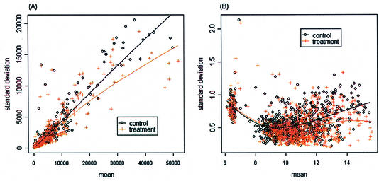
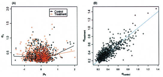
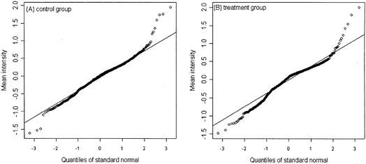
Figure 1A and B are scatterplots of the mean versus standard deviation of the un-normalized intensities for the control and treatment among the 705 genes, and the fitted lowess regression curves for the control and treatment samples. Figure 1A shows an approximately linear relationship between the mean and standard deviation before the log-transformation. Applying the log-transformation to stabilize variation, Figure 1B shows no apparent relationship between the mean and standard deviation. Figure 2A is a scatterplot of the mean versus standard deviation of the normalized intensities for the two groups. There is no apparent relationship between the mean and standard deviation. Figure 2B is a scatterplot of the standard deviations between the control versus the treatment. The standard deviations between the two groups for the 705 genes mostly appear to be similar. We also evaluated the correlation between two intensities on the same spot. The mean correlations for the un-normalized data and normalized data are 0.6 and 0.8, respectively; a significant correlation between two samples from the same spot. A normal probability plot is used to assess the normality assumption for this data set. A normal probability plot displays the ordered values of the data set versus the corresponding quantiles of a standard normal distribution. A linear plot would imply that the data are reasonably normal. Figure 3A and B are the normal probability plots for the control and treatment, respectively. It can be seen that the normalized intensity data appear to be heavy-tailed; this suggests that the data are more similar to a t-distribution than to a normal distribution. Using a permutation test to identify differentially expressed genes should be more appropriate.

Figure 1.

Scatterplots for mean intensity and standard deviation of background-subtracted and un-normalized data (described in Example data set). (A) An approximately linear relationship for non-transformed data. (B) Stabilized standard deviations, no apparent relationship between the mean and standard deviation for log-transformed data.

Figure 2.

Scatterplots for the example data set after a normalization. (A) Mean intensity versus standard deviation plot for control and treatment samples. There is no apparent relationship between the mean and standard deviation for the normalized log-intensity data. (B) Standard deviation plots of the control versus treatment. The standard deviations between the two groups are approximately equal.

Figure 3.

Normal probability plots of the normalized log mean intensity data for the control (A) and treatment (B) for the example data set. The normalized log intensities have heavy tails deviating from the normal variate.

RESULTS

Analysis of example data set

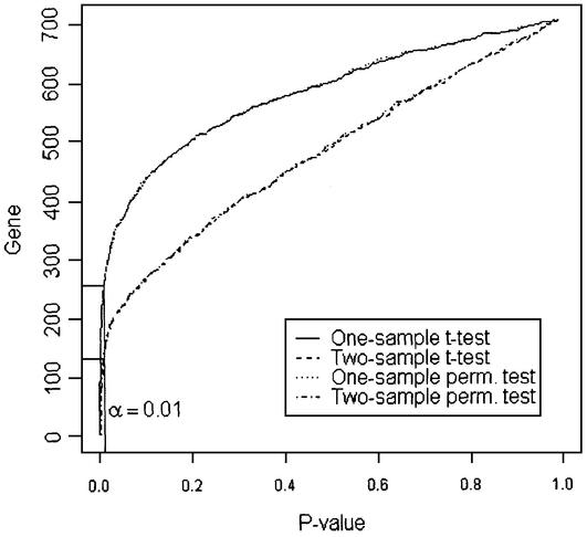
The control and treated groups are compared one gene at a time using the one- and two-sample t-tests, and one- and two-sample permutation t-tests. Figure 4 displays the p-values of the 700 genes with excluding five housekeeping genes for the four tests. If there is no treatment effect for all genes, i.e. all null hypotheses are true, then the p-values should be uniformly distributed on the interval (0,1). That is, the p-value plot should be a straight line across the diagonal. If a null hypothesis is not true, then its p-value will tend to be small. In Figure 4, the horizontal line at the y-axis represents the number of significant genes at the correspondent level of significance α = 0.01 (vertical line). Figure 4 shows that the distribution of p-values appears to be quite non-uniform and the numbers of significant genes from one-sample tests and two-sample tests are substantially different. However, the behaviors of one-sample t-test and permutation test are very similar, as are the two-sample t-test and the two-sample permutation test. Moreover, the one-sample t-tests appear more powerful than the two-sample t-tests because of a positive correlation between the control and treated samples on the same array.

Figure 4.

P-value plot for the four statistical tests on the example data set. Using the significance level at α = 0.01, the numbers of significant genes are 254, 257, 145 and 132 for one-sample t-test, one-sample permutation test, two-sample t-test and two-sample permutation test, respectively.

Simulation study

We conducted a Monte Carlo simulation experiment to evaluate the type I error of four methods for a control and treatment comparison. We generated gene expression levels under Models I–IV with r arrays per group, where r = 3, 5 and 8, and the number genes of in an array is g = 500 and 1000. We assumed an equal variance for the control and treated groups, φ²_ic = φ²_it = φ² and σ²_ic = σ²_it = σ². The true expression levels µ_ik for each channel at each spot were randomly drawn from a log-normal (base 2) distribution with mean 10 and the standard deviation 1.2 suggested by Hoyle et al. (19). This is based on 16-bit tiff images with the intensities ranging from 0 to 2¹⁶–1 (from 0 to 65 535). The parameter values of bivariate normal distribution (η_ijc,η_ijt) were φ² = 0.1 and 0.3 with the correlation τ_i = 0.9 and 0 (one-channel experiment). The parameter values of bivariate normal distribution (ε_ijc,ε_ijt) were σ² = 0.5 and 1, and ρ_i = 0.1 and 0 with the constraint τ_i ≥ ρ_i. For each simulated data set, the proportion of significances was calculated for the four methods at significance level α = 0.01. One thousand random samples were generated in each analysis. Note that the one-sample permutation test was based on 10 000 random samples from the population of all permutations. All simulations were carried out using Fortran 90 programs on Unix systems.

Table 1 is the average of the proportions of significances for g = 500 and r = 5. Since data from Model III and Model IV give similar results, only the results from Model IV are shown. It can be seen that for τ > 0 or ρ > 0 (correlated model), both the two-sample parametric and two-sample permutation t-tests are conservative. In particular, the two-sample permutation test is very conservative because of small sample sizes. (The averaged proportions of rejections for all models are zero for r = 3, not shown.) Both one-sample parametric and one-sample permutation t-tests perform well, with few exceptions. Table 2 is the averaged proportions of significance for g = 500 with r = 8. The tests show an overall improvement, as compared with r = 5; the averaged rejections are close to 0.01 for the two-sample permutation test with τ = 0 and ρ = 0 (independent model). The results for g = 1000 and r = 8 are similar (not shown). In summary, the one-sample parametric and one-sample permutation tests are similar, and two-sample parametric and two-sample permutation tests are similar with r = 8. When the data are correlated, both the parametric and permutation two-sample tests are too conservative because the assumption of independence is violated.

Table 1. Average type I errors of the one-sample (one-t) and two-sample (two-t) t-test, one-sample random permutation (one-p) and two-sample permutation (two-p) test under three statistical models for g = 500 and r = 5 at α = 1%.

		Model I				Model II				Model IV
(φ2,τ)	(σ2,ρ)	one-t	one-p	two-t	two-p	one-t	one-p	two-t	two-p	one-t	one-p	two-t	two-p
(0.1,0.9)	(0.5,0.0)	0.0100	0.0122	6.6E-5	6.4E-5	0.0095	0.0107	0.00	0.00	0.0099	0.0101	0.0068	0.0055
(0.1,0.9)	(0.5,0.1)	0.0101	0.0125	6.4E-5	5.0E-5	0.0041	0.0099	0.00	0.00	0.0099	0.0101	0.0054	0.0044
(0.1,0.0)	(0.5,0.0)	0.0101	0.0102	0.0100	0.0079	0.0109	0.0110	0.0090	0.0070	0.0101	0.0102	0.0101	0.0080
(0.1,0.9)	(1,0.0)	0.0103	0.0127	5.2E-5	4.2E-5	0.0045	0.0098	0.00	0.00	0.0100	0.0100	0.0079	0.0064
(0.1,0.9)	(1,0.1)	0.0101	0.0125	6.8E-5	4.8E-5	0.0107	0.0081	0.00	0.00	0.0099	0.0101	0.0063	0.0051
(0.1,0.0)	(1,0.0)	0.0100	0.0101	0.0101	0.0080	0.0090	0.0083	0.0090	0.0074	0.0101	0.0103	0.0098	0.0079
(0.3,0.9)	(0.5,0.0)	0.0102	0.0124	7.4E-5	8.6E-5	0.0092	0.0153	0.00	0.00	0.0098	0.0102	0.0037	0.0031
(0.3,0.9)	(0.5,0.1)	0.0100	0.0124	7.0E-5	5.8E-5	0.0141	0.0134	0.00	0.00	0.0099	0.0103	0.0030	0.0025
(0.3,0.0)	(0.5,0.0)	0.0099	0.0100	0.0100	0.0080	0.0100	0.0150	0.0150	0.0110	0.0099	0.0100	0.0098	0.0078
(0.3,0.9)	(1,0.0)	0.0097	0.0121	7.2E-5	5.6E-5	0.0062	0.0089	0.00	0.00	0.0101	0.0104	0.0057	0.0046
(0.3,0.9)	(1,0.1)	0.0101	0.0124	6.2E-5	5.0E-5	0.0091	0.0103	0.00	0.00	0.0101	0.0103	0.0045	0.0036
(0.3,0.0)	(1,0.0)	0.0099	0.0100	0.0098	0.0080	0.0090	0.0109	0.0099	0.0099	0.0100	0.0100	0.0099	0.0080

Table 2. Average type I errors of the one-sample (one-t) and two-sample (two-t) t-test, one-sample random permutation (one-p) and two-sample permutation (two-p) test under three statistical models for g = 500 and r = 8 at α = 1%.

		Model I				Model II				Model IV
(φ2,τ)	(σ2,ρ)	one-t	one-p	two-t	two-p	one-t	one-p	two-t	two-p	one-t	one-p	two-t	two-p
(0.1,0.9)	(0.5,0.0)	0.0100	0.0105	4.0E-6	4.0E-6	0.0061	0.0068	0.00	0.00	0.0099	0.0101	0.0060	0.0061
(0.1,0.9)	(0.5,0.1)	0.0100	0.0104	4.0E-6	4.0E-6	0.0112	0.0126	0.00	0.00	0.0100	0.0101	0.0043	0.0043
(0.1,0.0)	(0.5,0.0)	0.0097	0.0099	0.0100	0.0099	0.0130	0.0131	0.0110	0.0121	0.0101	0.0101	0.0099	0.0098
(0.1,0.9)	(1,0.0)	0.0100	0.0105	1.0E-5	1.2E-5	0.0092	0.0102	0.00	0.00	0.0101	0.0101	0.0078	0.0076
(0.1,0.9)	(1,0.1)	0.0099	0.0103	1.2E-5	1.2E-5	0.0111	0.0107	0.00	0.00	0.0100	0.0100	0.0055	0.0055
(0.1,0.0)	(1,0.0)	0.0101	0.0100	0.0101	0.0100	0.0090	0.0091	0.0108	0.0118	0.0100	0.0101	0.0101	0.0101
(0.3,0.9)	(0.5,0.0)	0.0101	0.0106	8.0E-6	6.0E-6	0.0169	0.0157	0.00	0.00	0.0099	0.0100	0.0028	0.0028
(0.3,0.9)	(0.5,0.1)	0.0099	0.0103	4.0E-6	4.0E-6	0.0043	0.0072	0.00	0.00	0.0099	0.0101	0.0021	0.0021
(0.3,0.0)	(0.5,0.0)	0.0099	0.0101	0.0099	0.0098	0.0070	0.0081	0.0070	0.0070	0.0103	0.0104	0.0098	0.0098
(0.3,0.9)	(1,0.0)	0.0099	0.0103	2.0E-6	4.0E-6	0.0090	0.0098	0.00	0.00	0.0101	0.0103	0.0051	0.0051
(0.3,0.9)	(1,0.1)	0.0100	0.0104	4.0E-6	6.0E-6	0.0092	0.0096	0.00	0.00	0.0101	0.0102	0.0037	0.0036
(0.3,0.0)	(1,0.0)	0.0100	0.0101	0.0101	0.0100	0.0100	0.0109	0.0142	0.0160	0.0102	0.0102	0.0102	0.0101

We conducted another simulation by varying the distribution of errors. The multiplicative errors (η_ijc,η_ijt) were drawn from a bivariate t-distribution with mean 0, degree of freedom 3 and correlation τ. For Models I and II, the additive errors (ε_ijc,ε_ijt) were drawn from a bivariate normal distribution with mean 0, variance σ²_c = σ²_t = 0.3 and correlation ρ. For Models III and IV, the additive errors were from the same bivariate t-distribution as (η_ijc,η_ijt) with correlation ρ. Table 3 is the average of the proportion of significance for r = 3, 5 and 8. It can be seen that the parametric tests, which rely on the normality assumption, are too conservative. The one-sample permutation test appears to perform well for r = 5 and 8; the test becomes conservative for r = 3 because of small sample size.

Table 3. Average type I errors of the one-sample (one-t) and two-sample (two-t) t-test, one-sample random permutation (one-p) and two-sample permutation (two-p) test under three statistical models for g = 500 and r = 3, 5 and 8 at α = 1% with (η_ijc = η_jt) drawn from a bivariate t-distribution with degree of freedom 3 and correlation τ.

		Model I				Model II				Model IV
r	(τ,ρ)	one-t	one-p	two-t	two-p	one-t	one-p	two-t	two-p	one-t	one-p	two-t	two-p
3	(0.9,0.0)	0.0075	0.0006	0.0004	0.00	0.0101	0.0006	0.00	0.00	0.0080	0.0004	0.0031	0.00
	(0.9,0.1)	0.0075	0.0006	0.0005	0.00	0.0062	0.0007	0.0020	0.00	0.0084	0.0005	0.0027	0.00
	(0.0,0.0)	0.0079	0.0006	0.0067	0.00	0.0088	0.0006	0.0110	0.00	0.0080	0.0005	0.0066	0.00
5	(0.9,0.0)	0.0065	0.0110	8.2E-5	8.4E-5	0.0040	0.0098	0.00	0.00	0.0073	0.0096	0.0017	0.0019
	(0.9,0.1)	0.0064	0.0110	4.4E-5	9.0E-5	0.0070	0.0096	0.00	0.00	0.0072	0.0095	0.0014	0.0016
	(0.0,0.0)	0.0070	0.0100	0.0061	0.0077	0.0042	0.0094	0.0070	0.0079	0.0072	0.0095	0.0066	0.0074
8	(0.9,0.0)	0.0064	0.0092	1.0E-5	1.4E-5	0.0080	0.0158	0.00	0.00	0.0072	0.0088	0.0011	0.0016
	(0.9,0.1)	0.0063	0.0090	6.0E-6	1.0E-5	0.0050	0.0101	0.00	0.00	0.0070	0.0090	0.0010	0.0012
	(0.0,0.0)	0.0071	0.0102	0.0069	0.0100	0.0082	0.0128	0.0110	0.0150	0.0074	0.0100	0.0070	0.0095

For Model IV, the errors (ε_ijc,ε_ijt) are distributed analogously, with correlation ρ. For Model I and II, the additive errors are drawn from a bivariate normal distribution with mean 0, variance σ²_c = σ²_t = 0.3 and correlation ρ.

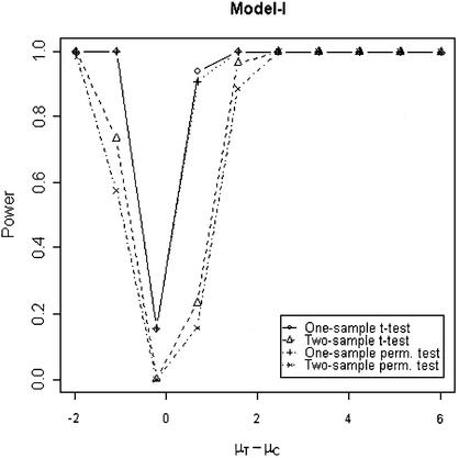
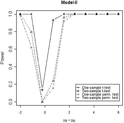
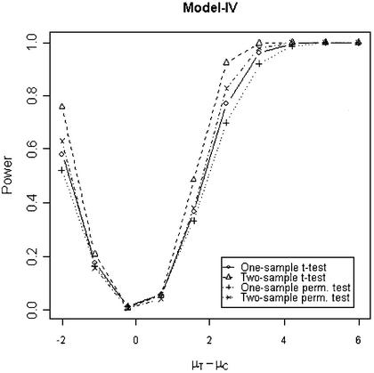
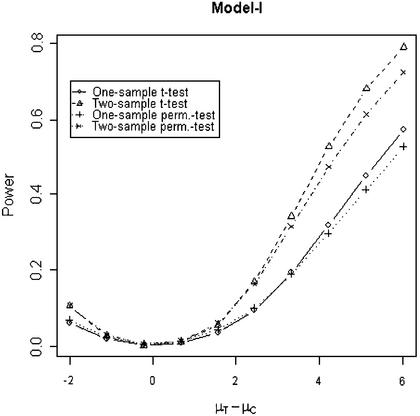
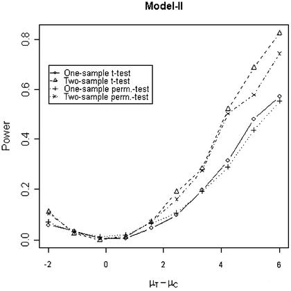
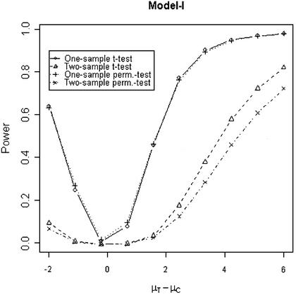
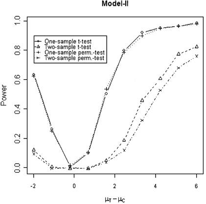
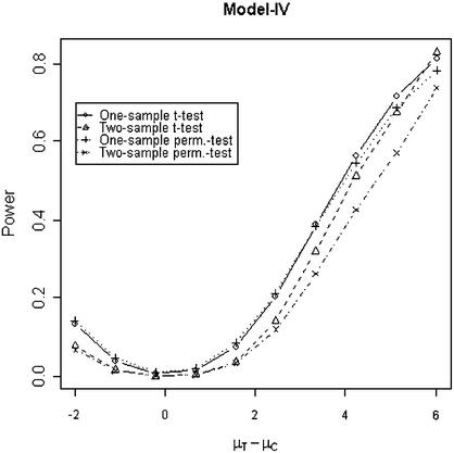
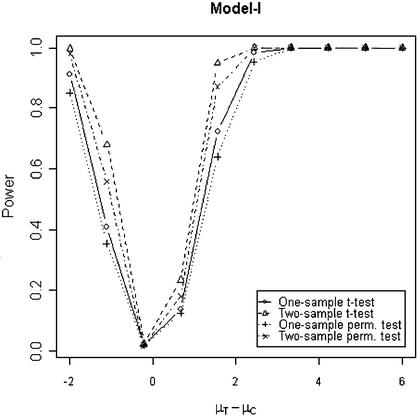
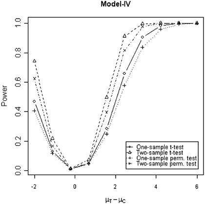
In addition to the type I error, we also examined the powers of the four tests for g = 500, r = 5 and µ_c = 9 shown in Figures 5–8. Figure 5 shows that the one-sample parametric and permutation tests are more powerful when the samples are correlated, as expected. Even when the data were generated from a t-distribution, the one-sample permutation test is more powerful than other tests (Fig. 7). When the two groups are independent, the two-sample parametric and permutation tests appear to be more powerful than one-sample tests for all three models (Figs 6 and 8). The permutation tests are as powerful as the parametric tests when r ≥ 5. In summary, when the data were generated from normal distributions with five replicates, the one-sample tests can detect a 2-fold change (in log scale) with >90% power and the two-sample test, under independence, can detect a 2-fold change with >95% power. When the data were generated from t-distributions, the powers are only 80% and 20% for one-sample and two-sample tests, respectively.

Figure 5.

Simulated power versus mean difference with µ_c = 9. The multiplicative errors (η_ijc,η_ijt) are drawn from a bivariate normal distribution with mean 0, variance φ²_c = φ²_t = 0.1 and correlation τ = 0.9. The additive errors (ε_ijc,ε_ijt) are generated analogously, with variance σ²_c = σ²_t = 0.5 and correlation ρ = 0.1.

Figure 8.

Simulated power versus mean difference with µ_c = 9. The multiplicative errors, η_ijc and η_ijt, are independently drawn from a t-distribution t(3) and the additive errors, ε_ijc and ε_ijt, are independently drawn from a t-distribution t(3) for Model IV and from a normal distribution N(0,0.3) for Model I and II.

Figure 7.

Simulated power versus mean difference with µ_c = 9. The multiplicative errors (η_ijc,η_ijt) are drawn from a bivariate t-distribution with degree of freedom 3 and correlation τ = 0.9. For Model IV, the additive errors (ε_ijc,ε_ijt) are generated analogously, with correlation ρ = 0.1. For Model I and II, the additive errors are drawn from a bivariate normal distribution with mean 0, variance σ²_c = σ²_t = 0.3 and correlation ρ = 0.1.

Figure 6.

Simulated power versus mean difference with µ_c = 9. The multiplicative errors, η_ijc and η_ijt, are independently drawn from a normal distribution N(0,0.1) and the additive errors, ε_ijc and ε_ijt, are independently drawn from a normal distribution N(0,0.5).

DISCUSSION

Intensity data from microarray experiments often involve a variety of random and systematic errors. In order to remove sources of variation, different transformation and normalization methods based on either raw or log-transformed intensity data have been proposed to adjust for stochastic biases. We use Models I and II to model raw expression data. The first order approximation of Model I is

X_ijc = µ_ic(1 + η_ijc + η²_ijc/2 + …) + ε_ijc = µ_ic + µ_ic · η_ijc + ε_ijc,

X_ijt = µ_it(1 + η_ijt + η²_ijt/2 + …) + ε_ijt = µ_it + µ_it · η_ijt + ε_ijt.

This model has been proposed by Ideker et al. (14). They used the likelihood ratio test approach to identifying differentially expressed genes. The computation of likelihood ratio test is not straightforward; it requires estimating the parameters of the bivariate normal models. In present evaluation, Tables 1–3 show that the log-transformed data from Models I or II can be analyzed using the traditional or permutation t-test. The tests seem to perform reasonably well in terms of type I error and power under proper conditions, for example, the two-sample permutation test performs well under an independent model. Models III and IV assume that the log-transformed normalized intensity data are normally distributed. Therefore, the t-test or permutation test can be applied directly. Models I and III assume the two sources of variation for spot intensities are independent. Models II and IV assume a systematic variation due to array-specific effects, such as amount of RNA or different hybridization dates, etc. Model IV may be more appropriate for some normalization methods, such as median or lowess, that are array dependent.

Because of lack of replications, the early approach for assessing differentially expressed genes is based on the ratio of the treatment-to-control to determine significant genes. This concept leads to the use of the one-sample t-test for the analysis of data from two-color dye-swap experiments. Alternatively, the two-sample t-test has also been used to detect genes with differential expression (9). This paper demonstrates that the two-sample t-test (either parametric or permutation test) is conservative when the samples are correlated (Example data set). For a two-color dye swap experiment, the one-sample tests appear to perform better than the two-sample tests. On the other hand, when the expression data are independent observations, such as one-channel microarray or two-channel reference design, the two-sample t-test is more powerful.

When the number of arrays is sufficient, the permutation test performs better than the corresponding parametric test when the data do not follow a normal distribution. In practice, the distribution of the normalized intensities appears to have a t-distribution rather than a normal distribution. With a small sample size, however, permutation tests can produce a skewed or bimodal reference distribution. For example, at replicate arrays r = 3, only 20 permutations are possible. When the number of replicates is small (r ≤ 3), the permutation test is not recommended.

The power study assumes a constant effect (mean difference) for all genes and evaluates the average proportion of significances of the given effect. In practice, the majority of genes do not express differentially between treatment groups. Furthermore, the genes that would be affected by a treatment generally have different effects. Different effects will result in different powers. However, the conclusions summarized above should remain valid.

REFERENCES

- 1.Chen J.J., Wu,R., Yang,P.C., Huang,J.Y., Sher,Y.P., Han,M.H., Kao,W.C., Lee,P.J., Chiu,T.F., Chang,F., Chu,Y.W., Wu,C.W. and Peck,K. (1998) Profiling expression patterns and isolating differentially expressed genes by cDNA microarray system with colorimetry detection. Genomics, 51, 313–324. [DOI] [PubMed]
- 2.Yang Y.W., Dudoit,S., Luu,P. and Speed,T.P. (2002) Normalization of cDNA microarray data: a robust composite method addressing single and multiple slide systematic variation. Nucleic Acids Res., 30, e15. [DOI] [PMC free article] [PubMed]
- 3.Irizarry R.A., Hobbs,B., Collin,F., Beazer-Barclay,Y.D., Antonellis,K.J., Scherf,U. and Speed,T.P. (2003) Exploration, normalization, and summaries of high density oligonucleotide array probe level data. Biostatistics, in press. [DOI] [PubMed]
- 4.Draghici S. (2002) Statistical intelligence: effective analysis of high-density microarray data. Drug Discov. Today, 7, S55–S63. [DOI] [PubMed]
- 5.Roberts C.J., Nelson,B., Marton,M.J., Stoughton,R., Meyer,M.R., Bennett,H.A., He,Y.D., Dai,H., Walker,W.L., Hughes,T.R., Tyers,M., Boone,C. and Friend,S.H. (2000) Signaling and circuitry of multiple MAPK pathways revealed by a matrix of global gene expression profiles. Science, 287, 873–880. [DOI] [PubMed]
- 6.Miller R.A., Galecki,A. and Shmookler-Reis,R.J. (2001) Interpretation, design, and analysis of gene array expression experiments. J. Gerontol. A. Biol. Sci. Med. Sci., 56, B52–B57. [DOI] [PubMed]
- 7.Newton M.A., Kendziorski,C.M., Richmond,C.S., Blattner,F.R. and Tsui,K.W. (1999) On differential variability of expression ratios: improving statistical inference about gene expression changes from microarray data. Technical report. University of Wisconsin, http://www.biostat.wisc.edu/geda/eba.html. [DOI] [PubMed]
- 8.Draghici S., Kuklin,A., Hoff,B. and Shams,S. (2001) Experimental design, analysis of variance and slide quality assessment in gene expression arrays. Curr. Opin. Drug Dis. Dev., 4, 332–337. [PubMed]
- 9.Dudoit S., Yang,Y.H., Callow,M.J. and Speed,T.P. (2002) Statistical methods for identifying differential expressed genes in replicated cDNA microarray experiments. Statistica Sinica, 12, 111–139.
- 10.Herwig R., Aanstad,P., Clark,M. and Lehrach,H. (2001) Statistical evaluation of differential expression on cDNA nylon arrays with replicated experiments. Nucleic Acids Res., 29, e117. [DOI] [PMC free article] [PubMed]
- 11.Wolfinger R.D., Gibson,G. and Wolfinger,E.D. (2001) Assessing gene significance from cDNA microarray expression data via mixed models. J. Comput. Biol., 8, 625–637. [DOI] [PubMed]
- 12.Black M.A. and Doerge,R.W. (2001) Calculation of the minimum number of replicate spots required for detection of significant gene expression fold change in microarray experiments. Technical Report. Department of Statistics, Purdue University. [DOI] [PubMed]
- 13.Chen Y., Dougherty,E.R. and Bittner,M.L. (1997) Ratio-based decisions and the quantitave analysis of cDNA microarray images. J. Biomed. Opt., 2, 364–374. [DOI] [PubMed]
- 14.Ideker T., Thorsson,V., Siegel,A.F. and Hood,L.E. (2000) Testing for differentially-expressed genes by maximum-likelihood analysis of microarray data. J. Comput. Biol., 7, 805–817. [DOI] [PubMed]
- 15.Rocke D.M. and Durbin,B. (2001) A model for measurement error for gene expression analysis. J. Comput. Biol., 8, 557–569. [DOI] [PubMed]
- 16.Chen Y.J., Kodell,R., Sistare,F., Thompson,K.L., Morris,S. and Chen,J.J. (2003) Normalization methods for cDNA microarray data analysis. J. Biopharm. Stat., 13, 57–74. [DOI] [PubMed]
- 17.Kerr M.K., Martin,M. and Churchill,G.A. (2000) Analysis of variance for gene expression microarray data. J. Comput. Biol., 7, 819–837. [DOI] [PubMed]
- 18.Kerr M.K., Afshari,C.A., Bennett,L., Bushel,P., Martinez,J., Walker,N.J. and Churchill,G.A. (2002) Statistical analysis of a gene expression microarray experiment with replication. Statistica Sinica, 12, 203–217.
- 19.Hoyle D.C., Rattray,M., Jupp,R. and Brass,A. (2002) Making sense of microarray data distributions. Bioinformatics, 18, 576–584. [DOI] [PubMed]