Disease contact tracing in random and clustered networks

Abstract

The efficacy of contact tracing, be it between individuals (e.g. sexually transmitted diseases or severe acute respiratory syndrome) or between groups of individuals (e.g. foot-and-mouth disease; FMD), is difficult to evaluate without precise knowledge of the underlying contact structure; i.e. who is connected to whom? Motivated by the 2001 FMD epidemic in the UK, we determine, using stochastic simulations and deterministic ‘moment closure’ models of disease transmission on networks of premises (nodes), network and disease properties that are important for contact tracing efficiency. For random networks with a high average number of connections per node, little clustering of connections and short latency periods, contact tracing is typically ineffective. In this case, isolation of infected nodes is the dominant factor in determining disease epidemic size and duration. If the latency period is longer and the average number of connections per node small, or if the network is spatially clustered, then the contact tracing performs better and an overall reduction in the proportion of nodes that are removed during an epidemic is observed.

1. Introduction

Contact tracing, or the identification of individuals that have been in contact with an infectious individual, is commonly used to identify newly infected cases, preferably before they become infectious. Contact tracing was used successfully in the control of the recent epidemic of severe acute respiratory syndrome (SARS; Lipsitch et al. 2003; Riley et al. 2003) and is also important in the control of sexually transmitted diseases (STDs; Clarke 1998; FitzGerald et al. 1998; Macke & Maher 1999). While in these examples contact tracing occurs at the individual level, in the case of foot-and-mouth disease (FMD), identification is at the group level; tracing of farming premises that have been in ‘dangerous contact’ (DC) with infected premises (IPs) is a central pillar of traditional disease control (Haydon et al. 2004). Contact tracing has had varied success in controlling disease. For SARS, contact tracing was considered to have been successful, although only a small proportion of quarantined persons actually had the disease. By contrast, contact tracing was considered to be ineffective in the recent 2001 FMD epidemic in the UK (Ferguson et al. 2001a,b; Keeling et al. 2001; Kao 2003), because resources were insufficient to identify and remove sufficient DCs quickly enough. When and why contact tracing is useful has been the subject of recent interest (Huerta & Tsimring 2002; Eames & Keeling 2003).

Motivated by the FMD epidemic, the problem of the efficacy of contact tracing on a network of farming premises is addressed, and those network- and disease-related properties that affect contact tracing efficiency are identified. Prior mathematical models of contact tracing on networks have considered disease structures where network nodes are considered to be susceptible (S), infectious (I), detected and triggering tracing (T) and either recovered and susceptible again (Eames & Keeling 2003) or removed (R; Huerta & Tsimring 2002). However, for many diseases there is a latent or exposed (E) stage; i.e. a significant delay before nodes become infectious, and this is the case for FMD IPs. As a latent stage should make contact tracing more effective (Fraser et al. 2004), we consider contact tracing on a network where the disease course includes latency.

Stochastic simulations and the moment closure method (Rand 1997) were used to analyse the epidemic dynamics. First, a network-based stochastic simulation is used, and thereafter, a deterministic model based on the moment closure approach is discussed and the results from the two different approaches are compared. We show conditions under which the introduction of the exposed group increases the efficiency of tracing. We also show conditions under which the main effect of contact tracing is to remove susceptible premises before they become infected, rather than removing exposed and/or IPs directly.

2. Methods: deterministic and stochastic models

(a) Epidemiological processes

Premises (farms, markets or livestock holdings) can be classified as belonging to one of five different disease states. Susceptible premises (S) hold only susceptible animals. Exposed premises (E) contain some animals incubating disease and possibly some that are infectious, but the numbers of infected animals are insufficient for it to be a likely source of infection. Infectious premises (I) hold sufficient infected animals that transmission is likely to occur; this may occur either by direct contact (movement of infected animals into susceptible premises) or indirect contact (transfer of virus without movement of infectious animals onto susceptible premises via equipment movement, aerosols or fomite transfer). While direct and indirect transmissions have distinguishing characteristics (in particular, time to infectiousness), it is assumed for the purposes of this study that these are the same. Positively diagnosed (e.g. by presence of clinical signs or diagnostic test) infectious premises (T) trigger DC tracing, are immediately isolated and no longer infectious. They are responsible for triggering primary tracing. Finally, removed premises (R) are those that have been isolated, either by removal of all susceptible animals or by quarantine prior to removal; they are no longer infectious and do not initiate tracing.

A logical way to model contact tracing among farms, markets and livestock holdings is to consider explicitly the underlying contact structure, i.e. the set of all the connections between the different premises. Each premises is then considered to be a node in a connected network of nodes. Consider N nodes and the set containing all the connections amongst them: the degree k of a node n is the total number of links between n and all the other nodes. If the nodes are distributed on a regular lattice, the degree of each node is the same; if the network is random, the degree distribution is Poisson with a mean degree K=〈k(n)〉.

If all the nodes are represented by their state in the above-mentioned five classes (SEITR), then the possible transitions between states are those presented in figure 1, and described below.

Figure 1.

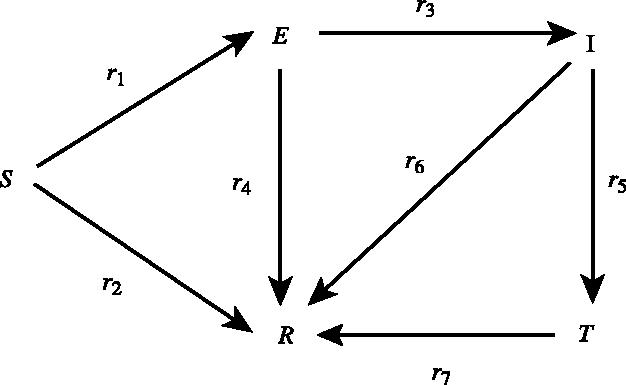
Possible transitions among the five different classes and the corresponding rates of transitions.

Infection S→E. The epidemic is seeded with one or more infected nodes. Thereafter, infection progresses as a simple contact process and the probability of a secondary infection depends on the state of the nodes that a specific node is in contact with. If a susceptible node has m infectious neighbours only, then the probability of becoming exposed during a time period of length Δt is given by 1−exp(−mr₁Δt), where r₁ is the rate at which susceptible nodes become exposed.

Tracing ‘errors’ S→R. Contact tracing may identify some contacts that were not truly infectious (e.g. animal movements where only uninfected animals were moved) at a given rate r₂. It is assumed that a node identified through contact tracing cannot initiate further tracing; i.e. ‘secondary’ tracing is suppressed. Therefore, a direct contact between a class (T) node and a susceptible node results in a susceptible node being traced and placed in the removed class (R). In the present model, tracing is assumed to be free from logistical constraints.

Becoming infectious E→I. This is the transition of the exposed nodes into the infectious class after the latency period has elapsed, and occurs at a prescribed rate r₃.

Tracing and removal of exposed nodes E→R. Exposed nodes in direct contact with class (T) nodes may be identified as potentially infectious and are removed at a prescribed rate r₄. As with tracing of class (S) nodes, this does not trigger further tracing.

Direct identification of infectious nodes I→T. Disease detected at an infectious node either through direct observation of clinical signs or via a diagnostic test will trigger tracing. r₅ is the transition rate of the infectious nodes into class (T) nodes and is a network-independent process.

Tracing of infectious nodes I→R. As with tracing of exposed nodes, tracing of infectious nodes does not trigger secondary tracing. While in principle further tracing might be triggered, for FMD in 2001, this was rarely the case. This process happens at rate r₆.

Removing or culling of class (T) nodes T→R. The removal of class (T) nodes with a given rate r₇. We assume that no further tracing occurs from a removed node. While this is not strictly true, the assumption simplifies the system, and the effect of continued tracing can be approximated by increasing the tracing rate from (T) class nodes. Further, late tracing is likely to be less important for this system, as many infected nodes would probably become positively diagnosed via clinical signs.

(b) Network structure

A connection or edge between two nodes implies that transmission from an infectious node to a susceptible one is possible. For FMD in 2001, it is well known that most transmission occurred over short distances, with only a few occurring at long range (Ferguson et al. 2001a,b). This can be interpreted as a clustering of connections, with probability of connection decreasing with distance. Thus, the nature of transmission will depend both on the number of contacts per node, and the clustering, and we shall consider both.

The disease transmission on networks is investigated in two ways: via stochastic simulation and a moment closure approximation. Stochastic simulations are implemented on random networks with average degree K=5, 7, 10, 15, 20 and N=2000 nodes. For each random graph, we ran multiple simulations starting each time with 10 different infectious nodes. The rates for the above-described transitions are: $r_1=(R_0^{\text{MF}}/K)/\text{Inf}\_P$, $r_2=(r_2^0/K)/\text{Tr}\_P$, $r_3=1/\text{Lat}\_P$, $r_4=(r_4^0/K)/\text{Tr}\_P$, $r_5=1/\text{Inf}\_P$, $r_6=(r_6^0/K)/\text{Tr}\_P$ and $r_7=1/\text{Tr}\_P$, where $r_i^0$ (i=1,…,7) are the different transition rates in the equivalent mean-field compartmental model. The basic reproduction ratio (R₀) is well known to be the average number of new infections resulting from the introduction of a single infected individual into a wholly susceptible population at equilibrium. Here, R₀^MF is the basic reproduction ratio in the mean-field model (R₀^MF<K). For individual-based network models, it has been shown (Keeling & Grenfell 2000) that R₀ is lower than for the mean-field equivalent; this is a result of the distributions of k and of the infectious period. The rates describing transitions are renormalized by a factor K to keep the transmission rate constant across different networks; however, we note that R₀ will be different across different networks with the same disease parameters. The parameters Inf_P and Lat_P are the average durations spent by nodes in the infectious and exposed states, respectively. Tr_P is the average duration spent by nodes in the (T) class. During this time, period neighbours of class (T) nodes are checked for possible infection. All the processes are considered to occur at the above-specified rates. The rates defined above are consistent with values appropriate to the recent FMD outbreak (Kao 2003).

The effect of varying Lat_P, r₂⁰, r₄⁰ and r₆⁰ is investigated on different random network configurations.

(c) The moment closure approximation

Let us denote by [S], [E], [I], [T] and [R] the number of nodes (i.e. the first moment) in any of the five classes at any time. The temporal dynamics of these variables is determined by the state of the nodes in the class that they are in direct contact with. To quantify this let [AB] denote the number of direct contacts between nodes in state A and B at any time across the entire network (i.e. the second moment). Likewise, [ABC] denotes the number of connected triplets (i.e. the third moment) where a node in state A is connected to a node in state B that is in turn connected to a node in state C. Considering the possible transitions presented in figure 1, the differential equations that describe the dynamics of the individual classes are

$$\begin{array}{l}[\dot{S}]=-r_1[SI]-r_2[ST],\hfill \\ [\dot{E}]=-r_3[E]-r_4[ET]+r_1[SI],\hfill \\ [\dot{I}]=-r_5[I]-r_6[IT]+r_3[E],\hfill \\ [\dot{T}]=-r_7[T]+r_5[I],\hfill \\ [\dot{R}]=r_2[ST]+r_4[ET]+r_6[IT]+r_7[T].\hfill \end{array}\}$$ 2.1

To solve these equations the time evolution of pairs of connected nodes are needed.

$$\begin{array}{l}[\dot{S}S]=-2r_1[SSI]-2r_2[SST],\hfill \\ [\dot{S}E]=-r_1[ISE]-r_2[TSE]-r_3[SE]-r_7[SET]+r_1[SSI],\hfill \\ [\dot{S}I]=-r_1[ISI]-r_2[TSI]-r_5[SI]-r_6[SIT]-r_1[SI]+r_3[SE],\hfill \\ [\dot{S}T]=-r_1[IST]-r_2[TST]-r_7[ST]-r_2[ST]+r_5[SI],\hfill \\ [\dot{E}E]=-2r_3[EE]-2r_4[EET]+2r_1[ISE],\hfill \\ [\dot{E}I]=-r_3[EI]-r_4[IET]-r_5[EI]-r_6[EIT]+r_1[ISI]+r_3[EE]+r_1[SI],\hfill \\ [\dot{E}T]=-r_3[ET]-r_4[TET]-r_7[ET]-r_4[ET]+r_1[IST]+r_5[EI],\hfill \\ [\dot{I}I]=-2r_5[II]-2r_6[IIT]+2r_3[EI],\hfill \\ [\dot{I}T]=-r_5[IT]-r_6[TIT]-r_7[IT]-r_6[IT]+r_3[ET]+r_5[II],\hfill \\ [\dot{T}T]=-2r_7[TT]-2r_5[IT].\hfill \end{array}\}$$ 2.2

The moment closure approach (Rand 1997) offers a sensible way of avoiding an infinite set of ordinary differential equations by ‘closing’ the system at the level of pairs and approximating triplets as a function of pairs and individual classes. For randomly connected networks, two different closure relations are commonly used. These differ according to the assumed error distribution under which the approximation is made. If this distribution of the error is Poisson, then the closure relation used is

$$[ABC]\approx \frac{[AB][BC]}{[B]}.$$ 2.3

If the distribution is similar to a Bernoulli distribution, then the approximation used is

$$[ABC]\approx \frac{K-1}{K}\frac{[AB][BC]}{[B]}.$$ 2.4

The closure relations (2.3) and (2.4) ignore the possible correlations between the node in state A and node in state C, which are both in direct contact with the same node in state B. These correlations are small if the network is random. However, in clustered networks there will be some heterogeneity in the probability of association between two nodes (in social networks, for example, the probability that two people will be friends will increase if they have a friend in common, or for FMD farms, are likely to have multiple common boundaries). To account for the correlation between the node in state A and node in state C, a modified closure relation is considered (Keeling 1999).

$$[ABC]\approx \frac{K-1}{K}\frac{[AB][BC]}{[B]}\left((1-\phi )+\phi \frac{N}{K}\frac{[AC]}{[A][C]}\right).$$ 2.5

Here, N is the number of nodes in the network, K is the average number of connections per node and φ is the clustering coefficient of the network. The parameter φ measures the degree of clustering in the network and is given by the ratio of triangles to triples, where triples are formed by any three nodes with exactly two connections amongst them, while triangles have three.

Since equations (2.1) and (2.2) are independent of [R], [SR], [ER], [IR], [TR] and [RR], it follows that the disease transmission problem can be approximated by a system of 14 deterministic ordinary differential equations.

(d) Stochastic simulations

The stochastic simulations were implemented using synchronous updating on computer-generated random and clustered networks. According to this method, the state of a node at the next time iteration (t₀+Δt) is solely based on the state of its neighbours (the nodes that are directly linked to it) at the current time (t₀) and the different rates according to which transitions between the classes occur. While the Gillespie algorithm (Gillespie 1977) is generally accepted to be the most efficient and appropriate method to stochastically represent systems such as the mean-field version of equation 2.1, it is likely that for the present system, the spatial correlations generated by synchronous updating are more realistic, because of the regular (daily) decision-making associated with contact tracing in our example. If the time-interval Δt used in the synchronous updating scheme is sufficiently small, then our scheme rapidly approaches the asynchronous updating scheme, where only one event happens during each iteration.

The generation of purely random networks is straightforward: networks were generated by assigning random probabilities to all the possible links, with only those links whose probability was smaller than a prescribed probability p included in the network. The average number of connections per node, K, is thus defined by pN. To generate clustered networks, we used the method described by Read & Keeling (2003). The nodes were distributed uniformly on a square of size $\sqrt{N}$ with their corresponding (x,y) coordinates. The distance-based connection probability between two nodes is given by $p_{ij}=p\text{exp}(-d_{ij}^2/2D^2)$, where d_ij is the Euclidean distance between node i and j, and p=K/2πD² if the system is infinite. Given the finite system size there will be a discrepancy between the prescribed and generated K. To obtain the prescribed K, a trial network is needed on which p is repeatedly readjusted until the generated network has an average number of connections per node equal to the desired K. The parameter D controls the clustering: D≈1 corresponds to highly clustered networks and D≈50 generates random networks with minimal levels of clustering. Multiple stochastic realizations of the epidemics were considered on the computer-generated random and clustered networks. The results were averaged over different networks and different realizations of the epidemic on each individual network. The number of networks and epidemic realizations to be averaged was determined by taking into account the differences between the consecutive averages of m and (m+1) single realizations, respectively.

3. Results

(a) Comparison of the stochastic and deterministic model for purely random networks

For random networks (no clustering), the closure relation (2.3) is used to explore the effects of different parameters. If K is sufficiently large, the closure relation (2.4) gives similar results to stochastic simulations. However, for small values of K, the first approximation has better agreement, and is therefore used hereafter. Figure 2 shows the time evolution of an epidemic from both stochastic simulations and numerical solutions of the moment closure equations for a fixed set of disease transmission parameters and K values. To stabilize the results, the epidemic is seeded with 10 randomly placed infected nodes; this results in the transient dip at the initial stages. Parameters are chosen to be reasonable for FMD transmission between farming premises. The discrepancies between the models are small for large values of K, corresponding to a more densely connected random network; however, if K is decreased, the agreement between the two models is less precise.

Figure 2.

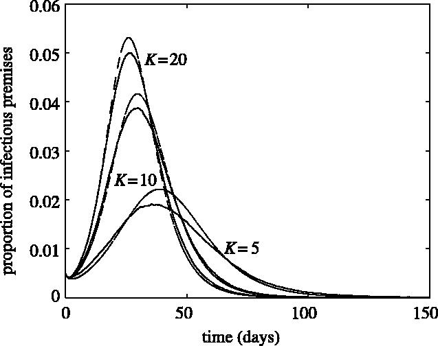
The time evolution of the epidemic from both stochastic (continuous lines) and deterministic (dashed lines) approaches for K=5, 10 and 20. The other parameter values are: R₀^MF=3.0, Inf_P=3.5, Lat_P=3.5, Tr_P=2.0, r₂⁰=2.5, r₄⁰=2.5 and r₆⁰=2.5.

(b) The efficacy of tracing

To investigate the effect of the exposed (E) class on the tracing efficiency, the final epidemic size $\left(\int r_{3}E(t)\text{d}t\right)$ is computed, using the deterministic model, for different average durations spent by nodes in the exposed state Lat_P. These computations are shown in figure 3 for random networks with different K values. As expected, increasing the duration of the exposed state (large Lat_P) reduces the final epidemic size due to the extra time available for tracing to identify and remove or isolate infected nodes quickly: preferably before they become infectious. This effect is much stronger for small K; if the average number of connections per node is reduced, removal of a connection reduces a greater proportion of the contact network, and so tracing efficiency increases. The higher the value of K, the less the impact of removal of a single connection.

Figure 3.

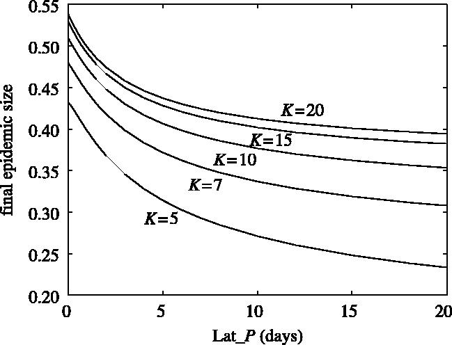
Final epidemic size $\left(\int r_{3}E(t)\text{d}t\right)$ corresponding to different latency periods (Lat_P). Results were obtained by solving differential equations (2.1) and (2.2) by first applying the closure relation (2.3). The other parameter values are: R₀^MF=3.0, Inf_P=3.5, Lat_P=3.5, Tr_P=2.0, r₂⁰=2.5, r₄⁰=2.5 and r₆⁰=2.5.

There are two mechanisms by which the potential size of an epidemic can be reduced. First, removal of susceptible nodes with rate r₂⁰ isolates infected nodes and limits disease spread. Second, removal of exposed and infectious nodes, with rate r₄⁰ and r₆⁰, respectively, shortens the transmission period of infected nodes. Here, we investigate the relative importance of these two mechanisms under more general network assumptions. Depending on the average number of connections per node (K) and the extent of the latency period Lat_P, we investigate the final size of the epidemic, the proportion of the susceptible nodes that were removed, the proportion of exposed and infectious nodes that were removed and the proportion of all the nodes eventually removed by the end of the epidemic (R(∞)), for a wide combination of the tracing rates. Since the average number of connections per node and the latency period has similar effects on disease contact tracing, only the two most contrasting cases are presented in the paper. First, in figures 4a and 5a the case of small K and large latency period is presented. Second, in figures 4b and 5b the case of large K and short latency period is discussed. While the first case represents optimal conditions for contact tracing, the second case makes contact tracing difficult. The case of small K and short latency period and the case of large K and long latency period are presented in the supplementary material section (see Electronic Appendix).

Figure 4.

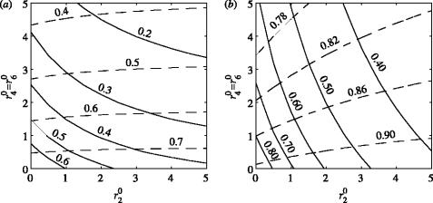
Contour plots of the final epidemic size, i.e. the proportion of all the nodes that eventually become infected during the epidemic (continuous lines) and R(∞), i.e. the proportion of all the nodes that were removed by the end of the epidemic (dashed lines). The two plots contrast the case of effective tracing (long latency period and few connections per node) with the case of less effective tracing (short latency periods and many connections per node). The other parameters used were: R₀^MF=3.0, Inf_P=3.5, Tr_P=2.0 and (a) K=5, Lat_P=10.0 and (b) K=20, Lat_P=3.5.

Figure 5.

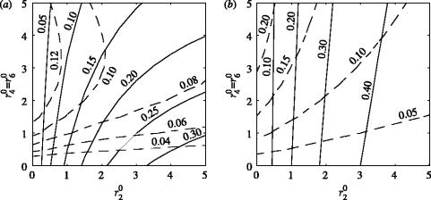
Contour plots of the proportion of both susceptible nodes (continuous lines) and exposed and infectious nodes (dashed lines) that were removed by tracing during the epidemic. The two plots contrast the case of effective tracing (long latency period and few connections per node) with the case of less effective tracing (short latency periods and many connections per node). The other parameters used were: R₀^MF=3.0, Inf_P=3.5, Tr_P=2.0 and (a) K=5, Lat_P=10.0 and (b) K=20, Lat_P=3.5.

Figure 4a,b show the final epidemic size (continuous lines) as a function of the removal rate of susceptible nodes r₂⁰ and the removal rate of exposed and infectious nodes r₄⁰=r₆⁰. For relatively few connections (small K) and long latency periods (large Lat_P; figure 4a), the final epidemic size is relatively small and is more sensitive to the removal of exposed and infected nodes than it is to the removal of susceptible nodes. In this case, a small increase in tracing (r₄⁰ and r₆⁰) has the same effect as a larger increase in the removal rate of susceptible nodes r₂⁰. With more connections and a shorter latency period (figure 4b), it is more difficult to control the epidemic and the final epidemic size is higher than in the previous case (figure 4a) and the removal of susceptible nodes becomes more important.

The total number of removed nodes or R(∞) is plotted (dashed line) in figure 4a,b. The removal of susceptible nodes has a limited effect on R(∞). While higher levels of tracing reduce the epidemic size, R(∞) stays the same owing to the higher proportion of susceptible nodes being removed. This suggests that if the average number of connections per node is sufficiently low and the latency period is sufficiently long, then contact tracing can efficiently control the final outcome of an epidemic by reducing the infectious period of infected nodes (preferably to zero). However, if K is too large or the latency period is too short, figure 4b shows that although the final size of the epidemic is similar to that in figure 4a, R(∞) is much higher: many nodes that were not infected were removed. Hence tracing, even if aimed primarily at removing exposed and infectious nodes, targets and removes susceptible nodes at a higher rate. Figure 5a,b shows contour plots of the proportions of both susceptible nodes and exposed plus infectious nodes that were removed through tracing. A higher proportion of susceptible nodes were removed on average through tracing, even in the case where the tracing of exposed and infectious nodes occurs at a much higher rate.

In figure 5a, more than one combination of tracing rates can result in the same number of nodes removed by tracing (e.g. at r₄⁰=1.35, r₄⁰=r₆⁰≈1.9 and r₄⁰=2, r₄⁰=r₆⁰≈3.4). This does not occur for the parameters in figure 5b, and is explained by the early extinction of the epidemic in the case where the tracing levels are higher. This illustrates the efficacy of contact tracing when K is small; in this case, even though R₀ is above one, high levels of tracing stop the epidemic early and with fewer nodes removed by tracing.

(c) Clustering effects

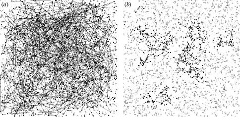
A randomly connected network will propagate disease much farther than a spatially clustered network, despite having the same average number of connections per node (figure 6; Watts & Strogatz 1998). In the randomly connected network, there are infected nodes throughout the system, whereas the highly clustered network shows localized, wave-like spread of the disease within a particular cluster of nodes.

Figure 6.

Final spatial spread of an epidemic for: (a) a random network with K=10, φ≈0 and (b) clustered network with K=10, φ≈0.50. The other parameters used were: R₀^MF=3.0, Inf_P=3.5, Lat_P=3.5, Tr_P=2.0, r₂⁰=2.5, r₄⁰=2.5 and r₆⁰=2.5. Empty circles represent susceptible nodes not affected by the disease and full circles are nodes that were removed by the end of the epidemic.

The disease dynamics and spread depend strongly on the local density of susceptible nodes. If the disease enters a cluster of susceptible nodes that are interconnected by short-range links, and there are only occasional long-range connections leading out of the cluster, it is plausible that the disease can be trapped within the cluster. Therefore, clustering means fewer susceptible nodes available for the disease to spread to. Occasionally, depletion of susceptible nodes in a cluster can stop the propagation of the disease in that specific area.

For clustered networks, the comparison between the results from the moment closure approach on using approximation (2.5) and stochastic simulations on clustered networks shows good agreement only if the level of clustering is sufficiently low (Levin & Durrett 1996). To capture accurately the effect of higher clustering, we use stochastic simulations hereafter to compute the final size of the epidemic and R(∞) for networks with different levels of clustering. The results are presented in figure 7. Contact tracing is considerably more effective in clustered networks and both the final epidemic size and R(∞) are much smaller compared with the random network case (Eames & Keeling 2003).

Figure 7.

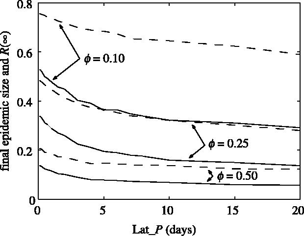
Final epidemic size (continuous lines) and R (∞; dashed lines) plotted for different latency periods (Lat_P) for different random spatially clustered networks. The other parameters used were: K=10, R₀^MF=3.0, Inf_P=3.5, Lat_P=3.5, Tr_P=2.0, r₂⁰=2.5, r₄⁰=2.5 and r₆⁰=2.5.

The probability of identifying a potentially dangerous node increases in clustered networks due to many different class (T) nodes linked to the same potentially dangerous individual within the cluster. Even if tracing from such a particular node fails to detect a potentially dangerous node, then tracing from another node within the cluster might still find it—tracing successfully shortens the transmission period of the traced node, even though the tracing did not occur via the infectious link. Figure 8 shows the proportion of the susceptible nodes and the proportion of exposed plus infectious nodes that were removed; in this case, the tracing rate of susceptible nodes (r₂⁰) is equal to the tracing rate of the exposed and infectious nodes r₄⁰=r₆⁰. Although the proportion of the removed nodes, in general, is smaller than in the random network case, the proportion of susceptible nodes that were removed is still higher than the proportion of infected (exposed plus infectious) nodes that were removed for this set of transition rates.

Figure 8.

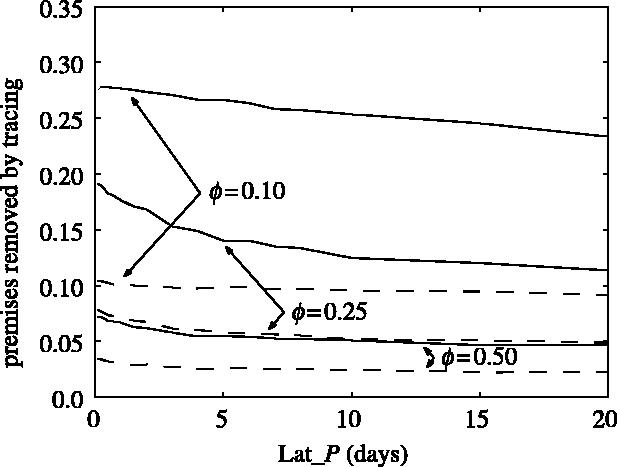
Plots of the final proportion of susceptible nodes (continuous lines) and exposed and infectious nodes (dashed lines) removed through tracing during the epidemic for different latency periods (Lat_P) for different random spatially clustered networks. The other values of the parameters are: K=10, R₀^MF=3.0, Inf_P=3.5, Lat_P=3.5, Tr_P=2.0, r₂⁰=2.5, r₄⁰=2.5 and r₆⁰=2.5.

4. Discussion

Contact tracing will inevitably involve the identification and removal of some nodes that are not infected. It is therefore important to know what proportion of the total population is removed via tracing, and how it relates to the proportion of exposed and infectious nodes that were removed, to the final epidemic size and to R(∞) for different contact structures and disease-specific parameters.

Figure 5 shows that the proportion of all the susceptible nodes removed through tracing represents a considerable part of the total removed population for all the parameter combinations considered, with the highest values obtained in the case of large K and short latency period. Thus, while not typically the intent of contact tracing, the dominant effect may be the removal of susceptible nodes even if nodes are connected at random over a large group (in this case, 2000 nodes). Removal of tracing's primary targets, exposed and infectious nodes, has only a secondary effect. Evaluation of disease control based on tracing must therefore consider the trade-off between the effort spent identifying infectious contacts, and the problems associated with removing a large number of uninfected nodes. For example, in the SARS epidemic (Lipsitch et al. 2003; Riley et al. 2003), many individuals were quarantined due to suspected contact with SARS. This was viewed as acceptable, both because of fears over the potential effects of a large epidemic, and because the impact on the quarantined individuals was relatively small. By contrast, in the FMD epidemic in the UK (Ferguson et al. 2001a,b; Keeling et al. 2001; Kao 2003), millions of animals were culled on farms suspected of harbouring FMD infection, and this was generally viewed as unacceptable.

The average number of connections per node, the degree distribution of the nodes and the degree of clustering are important in understanding the value of contact tracing and how different epidemiological mechanisms interact. Therefore, during an epidemic, any information that can be inferred about these quantities is valuable in assessing or deciding upon the most effective measures that can control an epidemic, and these are discussed in greater detail below.

If most connections are short-distance, premises close to each other can form multiply connected clusters with occasional long-range connections between clusters. The epidemic dynamics on such clustered networks are different in comparison to random networks. This extends the result of Eames & Keeling (2003) by showing that moderate clustering significantly increases the tracing efficacy, by considering only primary tracing. Secondary tracing is likely to enhance the impact of clustering, but it may not always be possible; for example, if logistical considerations limit the amount of tracing that can be done, effort is likely to be concentrated on finding primary contacts.

The length of the latency period is another factor that influences the effectiveness of tracing: longer latency periods allow more time for tracing, thus making it more effective. If infected nodes quickly become infectious, then the time for tracing is very short, and the value of tracing is less. While including secondary tracing (i.e. tracing from infected nodes identified via tracing) might affect our results, for FMD, secondary contact tracing did not occur unless existence of disease could be proven—in practice this almost never occurred. In any case, including secondary tracing in our model would only accentuate the differences between the two contact structure extremes (highly clustered connections with few contacts versus randomly connected with many contacts). Given the low impact of contact tracing in dense networks, the impact of secondary tracing is likely to be small.

While these results are generally valid for randomly connected networks or those in which clustering of contacts is important, FMD in the UK is the motivation for this work, and is discussed here in further detail. Soon after discovery of FMD in the UK in 2001, a national movement ban prevented almost all long-range livestock movements and most of the short-range ones, greatly reducing the range and rate of transmission (Ferguson et al. 2001a). However, new cases after the movement ban remained high, and therefore, revised policies to control disease were implemented. These policies proved controversial, with much of the criticism aimed at the ‘contiguous premises’ (CP) cull policy, to remove all premises contiguous to IPs within 48 h of disease identification. A major criticism was that many of these premises were uninfected and culled unnecessarily. It is also argued that the CP cull took resources away from the contact tracing that was already in place (discussed in Haydon et al. 2004). There has since been considerable scrutiny of the justification for the CP cull, in particular, aimed at the mathematical models that were used in ‘real time’ to advise policy. These models used both a moment closure approach (Ferguson et al. 2001a,b) and stochastic simulations (Keeling et al. 2001). While similar to the approach used here, in these FMD models, any IP is able to infect any susceptible premises and the probability of transmission decreases with distance. Other approaches (Morris et al. 2001) were more complicated, but relied on the same underlying transmission assumption. In the approach used here, the probability of transmission is equal for all connections, but the number of connections changes and for clustered networks there is a decreased probability of connection with distance. All the FMD models showed that the CP cull would be effective in reducing the final epidemic size. A related approach showed that the CP culling policy may have been more effective than a very good DC culling policy, but acknowledged that the result is likely to be model dependent (Kao 2003). Another study showed that the number of premises removed was insensitive to overculling, but favoured the CP cull because it reduced the number of IPs and the epidemic duration (Matthews et al. 2003).

A comparison between the FMD models and the model presented here can be made by observing that in Kao (2003), approximately 30% of transmission was assumed to occur to the six nearest neighbours, which is approximately equivalent to the number of available CPs, and is similar to the assumptions in other FMD models. If all susceptible premises were equally susceptible, removing a single susceptible CP would be equivalent to removing 5% of the susceptible neighbourhood, and in this sense it is roughly equivalent to tracing and removing a single connected susceptible node in a network with K=20. Removal of a correctly identified DC is equivalent to removing a single, connect and infected node. The FMD models are therefore similar to moderately clustered networks with high K values. Despite the differences in approach, our analysis illustrates why the CP cull was supported by the FMD models. Even with a significant latent period, in a densely connected network (see figures 1b and 2b in the Electronic Appendix), depletion of susceptible premises is more important than the early removal of infected premises. Whether or not CPs were truly at risk of infection is difficult to determine, and lies outside of this discussion, but we note that an examination of prior outbreaks of FMD in the UK suggests that transmission of virus between premises is not always as common as was supposed in 2001 (Haydon et al. 2004). If the true value of K was somewhat lower than suggested in the FMD models, this analysis suggests that contact tracing becomes more valuable than previously indicated (Kao 2003). Our results also confirm (figure 4) the findings of Matthews et al. (2003) regarding insensitivity to overculling, but also shows that this relationship breaks down provided the number of connections per node are sufficiently few, and the duration of the latency period sufficiently long (figure 5a). If this is the case, the extra effort of ‘good’ contact tracing can make a difference to the effectiveness of control.

Simple models are useful tools for analysing data and establishing hypotheses of disease transmission and control. They have the attractive feature that they are robust, and because of their abstract nature, the temptation to abuse them is reduced (May 2004). However, the increasing availability of powerful computers and the development of more sophisticated models can lead to model over-interpretation. Here, we have shown that decisions between control policies that rely on contact tracing depend on an accurate understanding of the contact structure that underlies disease transmission, determined through an analysis of data or independent experimental evidence.

References

- Clarke J. Contact tracing for chlamydia: data on effectiveness. Int. J. STD AIDS. 1998;9:187–191. doi: 10.1258/0956462981921945. [DOI] [PubMed] [Google Scholar]
- Eames K.T.D, Keeling M.J. Contact tracing and disease control. Proc. R. Soc. B. 2003;270:2565–2571. doi: 10.1098/rspb.2003.2554. 10.1098/rspb.2003.2554 [DOI] [PMC free article] [PubMed] [Google Scholar]
- Ferguson N.M, Donnelly C.A, Anderson R.M. The foot-and-mouth epidemic in Great Britain: pattern of spread and impact of interventions. Science. 2001;292:1155–1160. doi: 10.1126/science.1061020. [DOI] [PubMed] [Google Scholar]
- Ferguson N.M, Donnelly C.A, Anderson R.M. Transmission intensity and impact of control policies on the foot and mouth epidemic in Great Britain. Nature. 2001b;413:542–548. doi: 10.1038/35097116. [DOI] [PubMed] [Google Scholar]
- FitzGerald M.R, Thirlby D, Bedford C.A. The outcome of contact tracing for gonorrhea in the United Kingdom. Int. J. STD AIDS. 1998;9:657–660. doi: 10.1258/0956462981921305. [DOI] [PubMed] [Google Scholar]
- Fraser C, Riley S, Anderson R.M, Ferguson N.M. Factors that make an infectious disease outbreak controllable. Proc. Natl Acad. Sci. USA. 2004;101:6146–6151. doi: 10.1073/pnas.0307506101. [DOI] [PMC free article] [PubMed] [Google Scholar]
- Gillespie D.T. Exact stochastic simulation of coupled chemical reactions. J. Phys. Chem. 1977;81:2340–2361. [Google Scholar]
- Haydon D.T, Kao R.R, Kitching R.P. Opinion: the UK foot-and-mouth disease outbreak—the aftermath. Nat. Rev. Microbiol. 2004;2:675–681. doi: 10.1038/nrmicro960. [DOI] [PubMed] [Google Scholar]
- Huerta R, Tsimring L.S. Contact tracing and epidemics control in social networks. Phys. Rev. E. 2002;66 doi: 10.1103/PhysRevE.66.056115. (article number 056115.) [DOI] [PubMed] [Google Scholar]
- Kao R.R. The impact of local heterogeneity on alternative control strategies for foot-and-mouth disease. Proc. R. Soc. B. 2003;270:2557–2564. doi: 10.1098/rspb.2003.2546. 10.1098/rspb.2003.2546 [DOI] [PMC free article] [PubMed] [Google Scholar]
- Keeling M.J. The effects of local spatial structure on epidemiological invasions. Proc. R. Soc. B. 1999;266:859–867. doi: 10.1098/rspb.1999.0716. 10.1098/rspb.1999.0716 [DOI] [PMC free article] [PubMed] [Google Scholar]
- Keeling M.J, Grenfell B.T. Individual-based perspectives on R0. J. Theor. Biol. 2000;203:51–61. doi: 10.1006/jtbi.1999.1064. [DOI] [PubMed] [Google Scholar]
- Keeling M.J, et al. Dynamics of the 2001 UK foot and mouth epidemic: stochastic dispersal in a heterogeneous landscape. Science. 2001;294:813–817. doi: 10.1126/science.1065973. [DOI] [PubMed] [Google Scholar]
- Levin S.A, Durrett R. From individuals to epidemics. Phil. Trans. R. Soc. B. 1996;351:1615–1621. doi: 10.1098/rstb.1996.0145. [DOI] [PubMed] [Google Scholar]
- Lipsitch M, et al. Transmission dynamics and control of severe acute respiratory syndrome. Science. 2003;300:1966–1970. doi: 10.1126/science.1086616. [DOI] [PMC free article] [PubMed] [Google Scholar]
- Macke B.A, Maher J.E. Partner notification in the United States: an evidence-based review. Am. J. Prev. Med. 1999;17:230–242. doi: 10.1016/s0749-3797(99)00076-8. [DOI] [PubMed] [Google Scholar]
- Matthews L, Haydon D.T, Shaw D.J, Chase-Topping M.E, Keeling M.J, Woolhouse M.E.J. Neighborhood control policies and the spread of infectious diseases. Proc. R. Soc. B. 2003;270:1659–1666. doi: 10.1098/rspb.2003.2429. 10.1098/rspb.2003.2429 [DOI] [PMC free article] [PubMed] [Google Scholar]
- May R.M. Uses and abuses of mathematics in biology. Science. 2004;303:790–793. doi: 10.1126/science.1094442. [DOI] [PubMed] [Google Scholar]
- Morris R.S, Wilesmith J.W, Stem M.W, Sanson R.L, Stevenson M.A. Predictive spatial modeling of alternative control strategies for the foot-and-mouth disease epidemic in Great Britain. Vet. Rec. 2001;149:137–144. doi: 10.1136/vr.149.5.137. [DOI] [PubMed] [Google Scholar]
- Rand D.A. Theoretical ecology. vol. 2. Blackwell; Oxford: 1997. Correlation equations for spatial ecologies. [Google Scholar]
- Read J.M, Keeling M.J. Disease evolution on networks: the role of contact structure. Proc. R. Soc. B. 2003;270:699–708. doi: 10.1098/rspb.2002.2305. 10.1098/rspb.2002.2305 [DOI] [PMC free article] [PubMed] [Google Scholar]
- Riley S, et al. Transmission dynamics of the aetiological agent of severe acute respiratory syndrome SARS in Hong Kong: the impact of public health interventions. Science. 2003;300:1961–1966. doi: 10.1126/science.1086478. [DOI] [PubMed] [Google Scholar]
- Watts D.J, Strogatz S.H. Collective dynamics of ‘small-world’ networks. Nature. 1998;393:440–442. doi: 10.1038/30918. [DOI] [PubMed] [Google Scholar]
Associated Data
This section collects any data citations, data availability statements, or supplementary materials included in this article.