Space and stochasticity in population dynamics

Abstract

Organisms interact with each other mostly over local scales, so the local density experienced by an individual is of greater importance than the mean density in a population. This simple observation poses a tremendous challenge to theoretical ecology, and because nonlinear stochastic and spatial models cannot be solved exactly, much effort has been spent in seeking effective approximations. Several authors have observed that spatial population systems behave like deterministic nonspatial systems if dispersal averages the dynamics over a sufficiently large scale. We exploit this fact to develop an exact series expansion, which allows one to derive approximations of stochastic individual-based models without resorting to heuristic assumptions. Our approach makes it possible to calculate the corrections to mean-field models in the limit where the interaction range is large, and it provides insight into the performance of moment closure methods. With this approach, we demonstrate how the buildup of spatiotemporal correlations slows down the spread of an invasion, prolongs time lags associated with extinction debt, and leads to locally oscillating but globally stable coexistence of a host and a parasite.

The law of mass action, also called the mean-field assumption, was first introduced by Waage and Guldberg in 1864 (1), who related the rates of chemical reactions to the proportional amounts of the reacting substances. Volterra (2) brought the concept to ecology by interpreting Lotka’s model (3) of autocatalytic reaction in terms of predator–prey interactions. Since then, most mathematical models in ecology have been derived by using the mean-field assumption, i.e., by replacing local densities by global densities. In recent years, theoretical ecologists have attempted to overcome the assumption by constructing models that adequately capture spatial and stochastic population processes (4–10). One approach is moment closure (11) and the related methods of pair approximations (12, 13) and corrected mean-field models (14). These methods have been very widely used, and they have even provided the basis for advising policy concerning real epidemics (15). However, the assumptions of moment closure are justified by heuristic rather than mathematical arguments. Another approach is to derive stochastic equations by linearizing around a mean-field model (16, 17). This method has proved useful for the study of spatial autocorrelations and synchrony but is incapable of studying the impact of fluctuations, e.g., to mean densities. Here we present a previously undescribed theory that combines elements from both approaches and is able to capture the nonlinear effects of fluctuations without resorting to ad hoc assumptions. Our approach makes it possible to calculate exactly the corrections to mean-field models in the limit where the interaction range is large, and it provides insight into the performance of moment closure methods.

We develop our theory in the context of the spatial logistic model for point-like sessile individuals inhabiting d-dimensional continuous space. We assume that each individual produces offspring at a constant rate f and that the newborns disperse according to a dispersal kernel 𝒟. An individual at location x is assumed to have mortality rate μ + αΣ_i𝒞(x − x_i), where the parameters μ and α refer to density-independent and -dependent processes, the sum is taken over all individuals present at the time, and the kernel 𝒞 quantifies how competitive effects are distributed in space. We assume that both 𝒞 and 𝒟 are radially symmetric and normalized to integrate to unity over all space.

If interactions were global, the exact locations of the individuals would not matter, and in the case of infinitely many interacting individuals one would recover the deterministic mean-field model

where q⁽⁰⁾(t) describes the density of individuals at time t. In the spatial case, the equation in corrected to

where the additional term R(t) relates to the covariance between the density-dependent mortality rate and the distribution of individuals (see Methods). Equations such as Eq. 1 are called spatial moment equations (18), and they are an exact description of the underlying Markov process. Unfortunately, spatial moment equations are mathematically intractable, because they form an infinite hierarchy with each moment depending on higher-order moments. Consequently, an extensive body of literature (11, 19) has focused on developing moment closures to approximate the dynamics of second spatial moments, such as the term R(t), or more generally the function g(Δx, t, Δt), by which we denote the covariance between two samples of the population density, taken at times t and t + Δt with a spatial lag Δx (see Methods). Although moment closure methods can be used to supplement simulation studies, they rely fundamentally on the ultimately arbitrary choice of the closure. The best closure has been found not only to depend on the problem but also on the region of parameter space under consideration (11).

Systematic Perturbation Expansion

We can, however, proceed in a mathematically rigorous manner by developing a perturbation theory that assumes that the interactions act over a long but finite range. In other words, we may write

where L is the characteristic length scale involved in the interaction kernels, and the coefficients q⁽ⁱ⁾(t) can in principle be derived up to arbitrary order (see Methods for details). In Supporting Text and Table 1, which are published as supporting information on the PNAS web site, we compute the terms q⁽¹⁾(t) and q⁽²⁾(t) specifically for the spatial logistic model. The major advantage of the perturbative approach is that it becomes exact at the limit L → ∞, and that we know a priori that the error behaves as 𝒪(L^−(n+1)d), where n is the order of the approximation. Not surprisingly, the algebra involved in the computation of the higher-order terms becomes increasingly complex. We therefore also propose a previously undescribed moment closure scheme q̂(t), which captures the first-order term q⁽¹⁾(t) exactly, but summarizes the remaining terms by an approximation derived from the linearization of the underlying stochastic differential equation (20).

Denoting the Fourier transform with respect to the spatial variable by ·̃, the core of the approximation q̂(t) is given by the equations

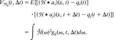
which describe how spatiotemporal correlations evolve in space and time. Whereas the variance of the noise V(t) works as the source, the term W̃(ω, t) describes how correlations are built up (due to dispersal) and dissolved (due to competition) at a given spatial frequency (see Methods). Knowledge of the function g(Δx, t, Δt) allows one not only to assess mean densities such as q(t), but also more localized quantities. For example, by defining the sampling variance V_ℋ(t, Δt) as the expected variance in population density within a sampling kernel ℋ (see Methods), it holds that

Examples

We next illustrate the general theory with three biological examples, in which we assume an exponential dispersal kernel and a “top-hat” competition kernel in the two-dimensional space. Denoting the characteristic length scales for dispersal and competition by L_𝒟 and L_𝒞, we define 𝒟(x) = e^−|x|/L_𝒟/(2π|x|L_𝒟), and 𝒞(x) = 1/(πL_𝒞²) if |x| ≤ L_𝒞 and 𝒞(x) = 0 if |x| > L_𝒞. Here we assume for simplicity that the two length scales are equal, although our method is not restricted to this case.

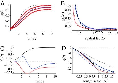
We first examine an invasion process in which a species increases from a low density toward the stationary state. Both during the invasion and at the stationary state, the spatial model predicts a lower density than the mean-field model (Fig. 1A). As spatial correlations build up (Fig. 1B), the local density experienced by a randomly selected individual becomes higher than the global density, and thus mortality is elevated over the mean-field level. The correlations are especially long-ranged in the invasive phase (blue line in Fig. 1B), during which the population grows patchily around initial foci (21, 22). Intriguingly, spatial correlations do not necessarily decay monotonically with distance but may become even negative (black line in Fig. 1B). This result is due to the shape of the top-hat competition kernel, which imposes strong competition at distances close to L_𝒞, at which the likelihood of dispersal is already limited. Fig. 1C shows that the first-order correction q⁽¹⁾(t) is always negative, but the second-order term q⁽²⁾(t) switches from positive to negative during the invasive phase. As expected, the inclusion of the first-order term leads to an asymptotically exact match with simulations, and the second-order term improves the quantitative match (Fig. 1D). The heuristic approximation q̂(t) is asymptotically exact to the first order and mimics the higher-order terms with reasonable success.

Fig. 1.

An invasion process. (A) The time evolution of the density of individuals based on the mean-field theory (dashed line), the first-order approximation (blue line), and the approximation q̂(t) (at this scale identical to the second-order approximation) ± one standard deviation (SD) of the sampling distribution (solid lines). The bars show the mean ± 2 standard errors from 250 simulation replicates, and the boxes show 1 SD among samples taken from Ω. (B) The spatial correlation function g [based on q̂(t) and simulations] is shown at times t = 1, 4, 10 (red, blue, and black lines). (C) The functions q⁽⁰⁾(t) (black line), q⁽¹⁾(t) (red line), and q⁽²⁾(t) (blue line). (D) The performance of various approximations against simulations at time t = 6. The black lines depict the purely perturbative approach taken to order 0 (dotted line), 1 (dashed line), and 2 (solid line). Red shows the approximation q̂(t), and the solid and dashed blue lines show the symmetric and asymmetric (4-1-1) power-2 moment closures, respectively. The simulations were run on a torus, the area of which was adjusted as a function of L in such a way that the expected number of individuals [according to q̂(t)] was 1,000. Parameters are as follows: f = 2, μ = 1, α = 1, L = L_𝒞 = L_𝒟 = 2, L_ℋ = 10. Initial density was Poisson distributed with q(0) = 1/10. Numerical integration in all figures was done by the classical Runge–Kutta method.

Law et al. (23) suggested that a particular asymmetric power-2 closure describes well the dynamics of the spatial logistic model under strongly aggregated patterns. They noted that although their closure works well in practice, it breaks down the sixfold symmetry of third moments, and should be seen as a convenient practical tool rather than rigorous theory. As shown in Fig. 1D, the closure of ref. 23 actually performs very poorly in the parameter regime we have studied, whereas the symmetric power-2 closure performs very well, as observed before (24). The present results give insight to the performance of existing moment closures: The symmetric power-1, -2, and -3 closures actually lead to an asymptotically exact approximation, capturing the first-order term q⁽¹⁾(t) correctly (as suggested by Fig. 1D), whereas the asymmetric closures fail to do so (Supporting Text). However, asymmetric closures have largely replaced symmetric closures because the latter often perform poorly with short-range interaction kernels (the opposite limit from the one we consider here). In our view, the insight given by such carefully tailored closures is limited, because they cannot be expected to behave robustly over a wide range of parameters. This limitation is illustrated by the poor performance of the closure of ref. 23, which was designed specifically for the spatial logistic model, but using different interaction kernels and different parameter values.

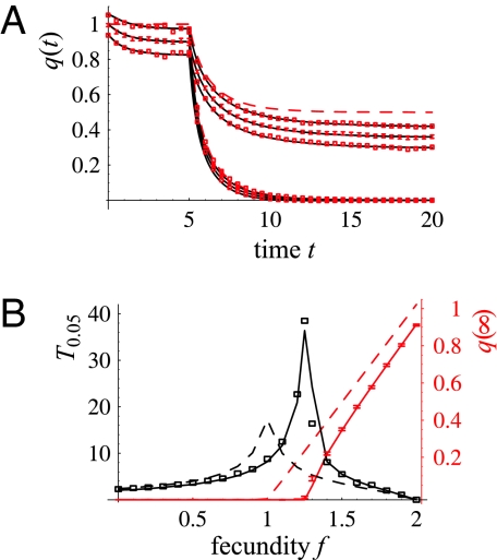
We next consider a situation in which a species declines after a sudden adverse change in the environment, caused, e.g., by habitat degradation or climate change. We assume that the environmental change causes a drop in the fecundity parameter f, which makes the species decline either to extinction or to a lower but positive stationary state (Fig. 2A). If the species declines below the extinction threshold, it is doomed to extinction, but the process will take some time. The number of species that have fallen below the extinction threshold but have not yet had time to go extinct has been called the extinction debt (25, 26), a concept that is fundamental in conservation (27, 28).

Fig. 2.

Decline after a sudden adverse environmental change. We assume that the parameter f of the species considered in Fig. 1 drops at time t = 5 to a lower value f̂. (A) The time evolution of the density of individuals with f̂ = 0.5 (lower lines) and f̂ = 1.5 (upper lines), with symbols as in Fig. 1A. (B) The black lines depict the length of the transient time T_0.05, measured as the time from t = 5 until the density of individuals first differs at most by 0.05 from the stationary density, |q(T_0.05) − q(∞)| < 0.05. The red lines show the equilibrium density q(∞). The dashed lines are based on the mean-field model, the solid lines represent the approximation q̂(t), and the boxes (depicting mean) and bars (depicting mean ± 2 standard errors) are based on 65 simulation replicates performed as in Fig. 1. Initial density was Poisson distributed with q(0) = 1.

Understanding the factors that affect the length of the transient period is a key component in the assessment of extinction debt. In the context of a spatial but deterministic metapopulation model, the length of the transient period T has been shown to depend on the magnitude of the change in the environmental conditions and on the species- and landscape-specific turnover rate of populations (29). Most importantly, the transient time depends on the distance to the extinction threshold, the transient being especially long if the long-term survival of the species is uncertain (29) (dashed lines in Fig. 2B). The individual-based spatial and stochastic model considered here adds one critical component to the formula of T: Species with distance-limited dispersal have a longer transient than species that disperse over long distances (solid lines in Fig. 2B). This finding is due to the fact that above and especially around the extinction threshold, the new stationary state involves strong long-range correlations that take time to build up.

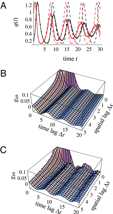
The theory that we have developed here in the context of the spatial logistic model generalizes to a wide range of spatiotemporal point process. For example, it can be used to study systems of n interacting species and dynamics that do not converge to a fixed point in the mean-field. To illustrate, we consider a spatial version of the Lotka–Volterra host–parasite model (see Methods). The mean-field model leads to cyclic dynamics, where both the amplitude and the frequency of the cycles depend on the initial condition for an infinitely long time. Although the spatial model initially follows the mean-field, small random fluctuations develop gradually into spatial asynchrony, which leads to statistical stabilization (30) of the mean density (Fig. 3A). However, locally the dynamics also continue to be cyclic at the stationary state (Fig. 3 B and C), the characteristics of which are independent of the initial state in contrast to the mean-field prediction. Local synchrony extends over a considerable spatial scale, several times the characteristic dispersal distance, and locally the signal of periodicity remains strong over several cycles (Fig. 3 B and C). Similar qualitative results have been obtained before for predator–prey systems (7, 31), the main difference being that our results are asymptotically exact in the sense discussed above. As illustrated in Fig. 3, the match between simulations and our analytical results is indeed very good.

Fig. 3.

Host–parasite dynamics. (A) The time evolution of the density of hosts (red) and parasites (black). The dashed lines show the mean-field prediction, and the solid lines show the approximation q̂(t). The bars show the mean ± 2 standard errors from 100 simulation replicates run in a torus of area 5,000. (B and C) The spatiotemporal correlation function of the hosts (g_hh) is based on the approximation q̂(t) (B) and simulations (C), both continued from A to the period t ∈ [50, 70]. Parameter values are as follows: f = μ = 1, α = 2, 𝒫(x) = e^−|x|/L_𝒫/(2πL_𝒫), L_𝒫 = L_𝒟 = 1.5. Initial density was Poisson distributed with h(0) = 1, p(0) = 0.2.

Discussion

Although many processes in theoretical physics can be viewed to take place in a discrete lattice, it is often more natural to model ecological and evolutionary processes in continuous space. In the past decade, the emphasis in spatial ecology has shifted from cellular automata toward such spatiotemporal point processes in which interactions among individuals are described in terms of distance-dependent kernels. Unfortunately, the theoretical machinery developed in physics for lattice models (32, 33) does not apply to continuous-space models, and theoretical ecologists have developed a diverse set of approximative methods. As well as being related to moment closure methods, our perturbation expansion shares some features with other techniques for studying birth–death processes. The van Kampen system size expansion (34) and the Urn model used in ref. 17 both assume that individuals are well mixed within a large container or patch. Within our model, the role of the “container” is played by the interaction kernels, which effectively average the population over a volume of order L^d. However, previous series expansions in population dynamics have focussed on the linearized fluctuations about a mean-field limit and on the study of spatial autocorrelation functions (7, 16, 17). The impact of stochastic fluctuations on the spatially averaged population density requires the consideration of higher-order terms in the expansion, as shown in ref. 20.

The results of this work demonstrate that the analysis of continuous-space stochastic models is possible without resorting to ad hoc assumptions. Our perturbation technique might also be applicable to physical systems on a lattice if the particles’ motion or interactions extended over many lattice spacings, although the expansion would break down near a critical point because it requires the correlation length to not be larger than the interaction length. Although the systematic perturbation approach provides an arbitrarily accurate solution within its radius of convergence, the increasing complexity involved both in the algebra and in the numerics makes it difficult to go beyond the second-order theory. The approximation q̂(t), which can be viewed as a mixture of symmetric power-1 and power-2 closures, provides an alternative that is asymptotically exact and also performs reasonably well for relatively short-ranged interaction kernels. Because it is based on mathematical arguments rather than on a fit to simulations, it is expected to behave robustly over a wide range of models and parameter space.

Methods

We rewrite the spatial logistic model by associating with each individual a delta distribution, so that the state of the system is described by a(x, t) = Σ_iδ(x − x_i), where the sum runs over all individuals present at time t. We split the distribution of individuals as a(x, t) = q(t) + s(x, t), where q(t) = E[a(x, t)] is the expectation over stochastic realizations, and s(x, t) represents the stochastic fluctuations. We assume that the initial condition is drawn from a probability distribution that is homogeneous with respect to space, so that q(t) does not depend on x. In this notation, the second moments g(Δx, t, Δt) and R(t) and the sampling variance V_ℋ(t) are defined as

Systematic Perturbation Expansion.

The systematic perturbation expansion is based on the hierarchical set of spatial moment equations that describe the dynamics of the nth order moment with the help of moments up to order n + 1. Such equations are exact, and they have been derived in the moment closure literature. The key to our method is the observation that we can assess the leading order (in terms of 1/L^d) of the nth order central moment, which we define as

To do so, we extract from G_n a combination of lower-order moments in such a way that the residual term G_n* is smooth and vanishes as the maximum distance between the n points diverges. To illustrate, we describe here such a decomposition for the second, third, and fourth moments. For the second moment, this decomposition reads simply as

where the term with the delta distribution arises as the two points may coincide (x₁ = x₂). Similarly, we may write the third moment as

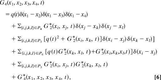
where the three permutations P = {{1, 2, 3}, {1, 3, 2}, {2, 3, 1}} correspond to the possibilities by which two of the three points may coincide. The fourth moment can be written as

where the permutations are defined as

Here the terms with the delta distributions refer again to cases in which some of the four points coincide. However, for the fourth moment and moments beyond that, it is not enough to account just for such singular terms. To see why this is the case assume that all of the four points are different but located so that x₁ and x₂ are close to each other, but far away from x₃ and x₄, which in turn are close to each other. In such a case, even if the distance between the two pairs of points diverges, the fourth moment will attain a nonzero value, which is captured in our decomposition by the term G₂*(x_i, x_j, t)G₂*(x_k, x_l, t). After the extraction of this term, it holds that G₄* vanishes as the maximum distance between the four points diverges, and the contribution from G₄* is of lower order. By ignoring G₄*, we can describe the dynamics of the third moment up to leading order, which in turn gives the dynamics of q(t) up to the order L^−2d. In general, ignoring the residual G_n* gives the dynamics of q(t) up to the order L^−(n−2)d. The rest of the derivation is basically algebra, in which the key is to drop systematically all terms that are of higher order than the one under construction. The resulting second-order expansion for the spatial logistic model and its derivation is given in full detail in Supporting Text.

Approximation q̂(t).

The Markov process can be written as the stochastic differential equation (20)

where dη represents spatial shot noise, the properties of which are determined by the underlying Markov process. As shown in Supporting Text, the covariance of the noise is given by

where V(t) is given by

By subtracting the expected value from both sides of Eq. 8 we find that the stochastic term satisfies

where Z = R − α(𝒞 ★ s)s. Because Z is a combination of a product and a convolution, the equation can not be solved in the closed form. We approximate Z by Z = −Rs/q, which can be justified by matching the expectation of Z both at points in which there is an individual and at points where there are no individuals (see below). Taking the Fourier transform f̃(ω) = ∫ f(x)e^−2πiωxdx gives

where Ã(ω, t) is given by

We define

Because the second moment does not depend on the absolute location, it holds that G̃(ω₁, ω₂, t, Δt) = g̃(ω₁, t, Δt)δ(ω₁ + ω₂). We obtain

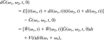from which Eq. 2 follows. Eq. 3 follows as

We next justify the approximation Z ≈ Z₀ = −Rs/q by showing that it captures the expected value of Z both at points in which there are and are not individuals. Let us first assume that a point x has been chosen randomly from R^d, in which case it is also (with probability 1) a point in which there is no individual. Because the point has been chosen randomly, E[(𝒞 ★ s)(x, t)] = 0. Because the point does not contain an individual, s(x, t) = −q(t). Thus, E[(𝒞 ★ s)(x, t)s(x, t)] = 0 and E[Z(x, t)] = R(t) = Z₀(x, t).

Let us then assume that the point x₀ has been chosen randomly among the locations of the individuals and restrict x here to a small neighborhood around the point x₀, so that s(x, t) = δ_x0(x) − q(t). Because αE[(𝒞 ★ s)s] = R(t) over the entire space, and because the expectation is zero excluding the locations of the individuals, we have αq(t)E[(𝒞 ★ s)(x₀, t)] = R(t). Thus, E[Z(x, t)] = −(R(t)/q(t))δ_x0(x) + 2R(t). Because Z₀(x, t) = −(R(t)/q(t))δ_x0(x) + R(t), Z₀ captures the expectation of Z (in the sense of a distribution, so the discrepancy in the constant does not count) in the small neighborhood around the point x₀.

Host–Parasite Model.

We assume that each host (h) individual produces offspring at a constant rate f, and the newborns are redistributed according to a dispersal kernel 𝒟. The parasite (p) attacks the hosts at rate α and with a kernel 𝒫, so that the rate at which a host individual at location x is turned into a parasite individual is α(𝒫 ★ p)(x). Hosts have no other mortality than that caused by the parasite, and parasites have a density-independent death rate μ. The mean-field model reads as

and leads to cyclic dynamics. In the spatial case, the equations are corrected to

where

and where g is the matrix of intra- and interspecific correlations

To derive the approximation (ĥ(t), p̂(t)), we write the Markov process as the coupled stochastic differential equation

To utilize vector notation, we define a = (h p)^T, q = E[a] = (q_h q_p)^T, s = a − q, and dη = (dη_h dη_p)^T. The covariance of the noise is given by

where

Proceeding as in the single species case and making the approximation

we obtain

where

Eq. 3 holds as such also in the matrix notation. We note that the sampling variance generalizes simply as

References

- 1.Waage P., Guldberg C. M. Forhandlinger: Videnskabs-Selskabet i Christiana; 1864. p. 35. [Google Scholar]
- 2.Volterra V. Variations and Fluctuations of the Number of Individuals in Animal Species Living Together. New York: McGraw–Hill; 1926. pp. 409–448. [Google Scholar]
- 3.Lotka A. J. J. Am. Chem. Soc. 1920;42:1595–1599. [Google Scholar]
- 4.Durrett R., Levin S. Theor. Popul. Biol. 1994;46:363–394. [Google Scholar]
- 5.Rand D. A., Wilson H. B. Proc. R. Soc. London Ser. B; 1995. pp. 111–117. [Google Scholar]
- 6.McGlade J., editor. Advanced Ecological Theory. Oxford: Blackwell Scientific; 1999. [Google Scholar]
- 7.Wilson W. G. Am. Nat. 1998;151:116–134. doi: 10.1086/286106. [DOI] [PubMed] [Google Scholar]
- 8.Pascual M., Levin S. A. Ecology. 1999;80:2225–2236. [Google Scholar]
- 9.Dieckmann U., Law R., Metz J. A. J., editors. The Geometry of Ecological Interactions: Simplifying Spatial Complexity. Cambridge, U.K.: Cambridge Univ. Press; 2000. [Google Scholar]
- 10.Lande R., Engen S., Saether B.-E. Stochastic Population Dynamics in Ecology and Conservation. Oxford: Oxford Univ. Press; 2003. [Google Scholar]
- 11.Murrell D. J., Dieckmann U., Law R. J. Theor. Biol. 2004;229:421–432. doi: 10.1016/j.jtbi.2004.04.013. [DOI] [PubMed] [Google Scholar]
- 12.Matsuda H., Ogita N., Sasaki A., Sato K. Prog. Theor. Phys. 1992;88:1035–1049. [Google Scholar]
- 13.Keeling M. J., Rand D. A., Morris A. J. Proc. R. Soc. London Ser. B; 1997. pp. 1149–1156. [Google Scholar]
- 14.Pascual M., Mazzega P., Levin S. A. Ecology. 2001;82:2357–2369. [Google Scholar]
- 15.Ferguson N. M., Donnelly C. A., Anderson R. M. Science. 2001;292:1155–1160. doi: 10.1126/science.1061020. [DOI] [PubMed] [Google Scholar]
- 16.Lande R., Engen S., Saether B. E. Am. Nat. 1999;154:271–281. doi: 10.1086/303240. [DOI] [PubMed] [Google Scholar]
- 17.McKane A. J., Newman T. J. Phys. Rev. E Stat. Phys. Plasmas Fluids Relat. Interdiscip. Top. 2004;70:041902. [Google Scholar]
- 18.Bolker B. M., Pacala S. W. Am. Nat. 1999;153:575–602. doi: 10.1086/303199. [DOI] [PubMed] [Google Scholar]
- 19.Filipe J. A. N., Gibson G. J. Bull. Math. Biol. 2001;63:603–624. doi: 10.1006/bulm.2001.0234. [DOI] [PubMed] [Google Scholar]
- 20.Ovaskainen O., Cornell S. J. Theor. Popul. Biol. 2006;69:13–33. doi: 10.1016/j.tpb.2005.05.005. [DOI] [PubMed] [Google Scholar]
- 21.Bolker B. M. Bull. Math. Biol. 1999;61:849–874. doi: 10.1006/bulm.1999.0115. [DOI] [PubMed] [Google Scholar]
- 22.Lewis M. A., Pacala S. J. Math. Biol. 2000;41:387–429. doi: 10.1007/s002850000050. [DOI] [PubMed] [Google Scholar]
- 23.Law R., Murrell D. J., Dieckmann U. Ecology. 2003;84:252–262. [Google Scholar]
- 24.Bolker B., Pacala S. W. Theor. Popul. Biol. 1997;52:179–197. doi: 10.1006/tpbi.1997.1331. [DOI] [PubMed] [Google Scholar]
- 25.Tilman D., May R. M., Lehman C. L., Nowak M. A. Nature. 1994;371:65–66. [Google Scholar]
- 26.Hanski I., Ovaskainen O. Conserv. Biol. 2002;16:666–673. [Google Scholar]
- 27.Hanski I. Ann. Zool. Fenn. 2000;37:271–280. [Google Scholar]
- 28.Berglund H., Jonsson B. G. Conserv. Biol. 2005;19:338–348. [Google Scholar]
- 29.Ovaskainen O., Hanski I. Theor. Popul. Biol. 2002;61:285–295. doi: 10.1006/tpbi.2002.1586. [DOI] [PubMed] [Google Scholar]
- 30.Briggs C. J., Hoopes M. F. Theor. Popul. Biol. 2004;65:299–315. doi: 10.1016/j.tpb.2003.11.001. [DOI] [PubMed] [Google Scholar]
- 31.Bolker B. M. Continuous-Space Models for Population Dynamics. London: Academic; 2004. pp. 45–69. [Google Scholar]
- 32.Dickman R. Phys. Rev. A. 1986;34:4246–4250. doi: 10.1103/physreva.34.4246. [DOI] [PubMed] [Google Scholar]
- 33.Oitmaa J., Hamer C., Zheng W. Series Expansion Methods for Strongly Interacting Lattice Models. Cambridge, U.K.: Cambridge Univ. Press; 2006. [Google Scholar]
- 34.Kampen N. G. Stochastic Processes in Physics and Chemistry. 2nd Ed. North–Holland, Amsterdam: 1992. [Google Scholar]
Associated Data
This section collects any data citations, data availability statements, or supplementary materials included in this article.