Simple models for containment of a pandemic

Abstract

Stochastic simulations of network models have become the standard approach to studying epidemics. We show that many of the predictions of these models can also be obtained from simple classical deterministic compartmental models. We suggest that simple models may be a better way to plan for a threatening pandemic with location and parameters as yet unknown, reserving more detailed network models for disease outbreaks already underway in localities where the social networks are well identified.

We formulate compartmental models to describe outbreaks of influenza and attempt to manage a disease outbreak by vaccination or antiviral treatment. The models give an important prediction that may not have been noticed in other models, namely that the number of doses of antiviral treatment required is extremely sensitive to the number of initial infectives. This suggests that the actual number of doses needed cannot be estimated with any degree of reliability. The model is applicable to pre-epidemic vaccination, such as annual vaccination programs in anticipation of an ‘ordinary’ influenza outbreak with limited drift, and as a combination of treatment both before and during an epidemic.

1. Introduction

The spread of a strain of avian influenza (H5N1) through Southeast Asia and parts of Europe has been causing much concern about pandemic influenza if the avian strain should develop into a strain with human-to-human transmission. Several recent studies, including Gani et al. (2005), Longini et al. (2004, 2005), Balicer et al. (2005) and Ferguson et al. (2005), have examined models to attempt to control such a pandemic influenza at the source should one develop. These recent models have been based on networks and stochastic simulations and have great potential for detailed predictions of outcomes and design of control strategies, especially for spatial spread. However, some of the model parameters have considerable uncertainty and such models are not very amenable to sensitivity analysis. The network models studied so far have been large-scale (500 000 people in Longini et al. 2005 and 85 000 000 people in Ferguson et al. 2005), and their predictions depend strongly on the specific location of an initial outbreak.

We suggest that as a general policy in preparing for an outbreak of a disease whose parameters are not yet known, it would be better to use a general compartmental model involving relatively few parameters and not depending critically on the particular as yet unknown setting. Perhaps the most appropriate use for this model is for a specific region in which a disease breaks out. As more becomes known about the nature of the disease, a more detailed network model can be used for more detailed analysis. For a new disease with no known treatment at the outset, the model described in Gumel et al. (2004), originally designed for the SARS epidemic of 2002–2003, serves as a template for evaluating the effects of quarantine and isolation. General templates for classes of diseases are appropriate for advance estimates of a possible epidemic before detailed information about a specific disease is available.

2. The basic model

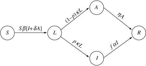
We develop a general epidemic model for a disease based on the standard SLIAR model (Brauer 2006), but including an additional property for influenza suggested in Longini et al. (2004), namely that some members of the population who are infected never develop symptoms but go directly from the latent stage to an asymptomatic infective stage and then to the removed stage. The model consists of a system of five ordinary differential equations with initial conditions for the number of susceptible (S(t)), latent, i.e. infected but not yet infective (L(t)), infective and symptomatic (I(t)), asymptomatic but infective (A(t)) and removed (R(t)) members. Initially, the total population size is K, of which a small number I₀ are infective and the remainder S₀ are susceptible, with S₀+I₀=K. A flow diagram for the model is shown in figure 1. We describe the predictions that may be made using this model and the model including treatment, which is described below. We leave the mathematical analysis of the models to the accompanying electronic supplementary material.

Figure 1.

SLIAR epidemic model.

It is not difficult to show that as t→∞, L(t), I(t) and A(t) each tends to zero and S(t) decreases monotonically to a limit S_∞>0. The basic reproduction number $\mathcal{R}$₀ is defined as the number of secondary infections caused by introducing a single infective into a susceptible population. Its value may be calculated using the method of Diekmann & Heesterbeek (2000) and van den Driessche & Watmough (2002) as

$${\mathcal{R}}_0=S_0\beta \left[\frac{p}{\alpha }+\frac{\delta (1-p)}{\eta }\right],$$ (2.1)

where β is the (constant) fraction of the population effectively contacted in unit time per individual, 1/α is the mean infective period, 1/η is the mean asymptomatic period, δ is the reduction in infectivity of asymptomatic members and p is the fraction of latent members that develop symptoms. It is convenient to define

$$\rho =\alpha \left[\frac{p}{\alpha }+\frac{\delta (1-p)}{\eta }\right],$$ (2.2)

so that

$${\mathcal{R}}_0=\frac{S_0\beta \rho }{\alpha }.$$ (2.3)

The expression ρ represents a correction factor in $\mathcal{R}$₀ that accounts for the presence of asymptomatic infectives. If ${\mathcal{R}}_0>1$, then the number of infectives first increases before decreasing to zero, while if ${\mathcal{R}}_0<1$, then the number of infectives decreases monotonically to zero. In preparing for an influenza epidemic, a range of basic reproduction numbers must be assumed, since the basic reproduction number cannot be known in advance.

The final size relation, essential for determining the total number of infections S₀−S_∞, is given by

$$S_0[\text{ln}{S}_0-\text{ln}{S}_{\infty }]={\mathcal{R}}_0(S_0-S_{\infty })+\frac{{\mathcal{R}}_0{I}_0}{\rho }.$$ (2.4)

This final size relation is valid for all $\mathcal{R}$₀, as it simply represents the orbit of the model (system (1) in the electronic supplementary material) as t→∞. Recall that for an epidemic model in which there are no demographic terms, I→0 as t→∞ for all orbits; ${\mathcal{R}}_0<1$ describes the case of no epidemic in which I tends monotonically to zero, while $\mathcal{R}$₀>1 describes the case of an epidemic in which I first increases to a maximum and then tends to zero.

The attack rate is defined as the fraction of the susceptible population that develops disease symptoms over the course of the epidemic. In our notation, this is p(1−S_∞/S₀). The basic reproduction number $\mathcal{R}$₀ is related to the attack rate through the final size relation. Using the disease parameters of Longini et al. (2004) for the 1957 influenza epidemic with a mean attack rate comparable to that assumed in Longini et al. (2004), our model gives $\mathcal{R}$₀=1.37, S₀β=0.40 and predicts 689 cases of disease in a population of 12 initial infectives and 1988 susceptibles (including the original 12 infectives), close to the 668 cases predicted by a stochastic simulation model in Longini et al. (2004).

3. The model with treatment

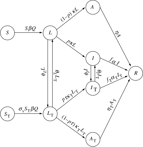
We also develop an extension that adds treatment to the model described above. Treatment can be vaccination, antiviral treatment before an epidemic or treatment of diagnosed infectives and/or latent members of the population identified by contact tracing during an epidemic. These assumptions require us to introduce additional compartments into the model to follow treated members of the population through the stages of infection. We use the classes S, L, I, A, R as before and introduce S_T(t), the number of treated susceptibles, L_T(t), the number of treated latent members, I_T(t), the number of treated infectives and A_T(t), the number of treated asymptomatics.

We assume that vaccination and antiviral treatment have the following benefits. They produce reductions in susceptibility and in infectivity, as well as a reduction in the fraction of latent members that will develop symptoms and a more rapid recovery and lower death rate of treated members. There are treatment rates φ_L of L and φ_I of I, respectively. We assume further that treatment does not change the initial contact rate S₀β, so that we may use the value of S₀β estimated in the untreated model for simulations that include treatment.

The resulting model, for which a flow diagram is shown in figure 2, is a system of nine differential equations. The treatment model with parameters comparable to those of Longini et al. (2004) predicts only 14 cases of disease on average, compared to the 46 cases predicted in Longini et al. (2004), table 2, with antiviral treatment of infectives and contacts. This predicted number is, however, very sensitive to changes in parameter values and the confidence interval in Longini et al. (2004) is large enough to include our number.

Figure 2.

Epidemic treatment model.

4. Results

We apply the model to the situation in which there is no pre-epidemic treatment, only treatment of latent and infective members of the population during the epidemic. In addition to the basic reproduction number $\mathcal{R}$₀, we consider a control reproduction number $\mathcal{R}$_c. The control reproduction number $\mathcal{R}$_c is defined as the number of secondary infections caused by introducing a single infective into a susceptible population with control measures in place, and its value may be calculated from the parameters of the model.

The final size relation for the treatment model is

$$S_0[\text{ln}{S}_0-\text{ln}{S}_{\infty }]={\mathcal{R}}_{\text{c}}(S_0-S_{\infty })+\frac{{\mathcal{R}}_0{I}_0}{{\rho }_{\text{T}}},$$ (4.1)

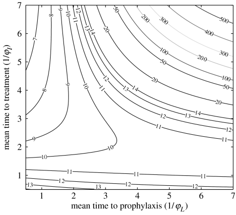
where ρ_T≥ρ is determined by the model parameters, with ρ_T=ρ if there is no treatment of infectives. An expression for the parameter ρ_T is given in the electronic supplementary material. The final size relation for the treatment model is valid for all $\mathcal{R}$₀ and $\mathcal{R}$_c. If $\mathcal{R}$_c<1, there is no epidemic for the treatment model, while if $\mathcal{R}$_c>1, there is an epidemic but eventually I tends to zero. As an example, figure 3 shows the contour lines of the number of doses (calculated from (10) in the electronic supplementary material and the number of doses used in the course of a treatment) as a function of the treatment parameters φ_L and φ_I in a population of 999 susceptibles and one infective if $\mathcal{R}$₀=1.5. The location of the curve $\mathcal{R}$_c=1 may be read from the figure; it runs approximately from the point (2.6, 7) to the point (7, 3.8) and is concave up. The curve $\mathcal{R}$_c roughly parallels the contour for 20 doses. As can be seen in figure 3, if $\mathcal{R}$_c≥1, estimates of the number of doses needed during an outbreak are very sensitive to parameter values. Note that the scale of the spacing of contour lines in figure 3 changes for contours below 20 and contours above 20.

Figure 3.

Total number of doses used in a population of 1000 individuals over the course of the outbreak as a function of the mean times to treatment and prophylaxis (in days), for $\mathcal{R}$₀=1.5, with S₀=999 and I₀=1.

We may estimate various combinations of treatment rates of latent and symptomatic members required to bring $\mathcal{R}$_c down below 1. As is shown in figure 3, this is feasible for $\mathcal{R}$₀=1.5, but may not be possible for larger values of $\mathcal{R}$₀. This possibility also depends on the availability of facilities to carry out the level of treatment required. In practice, epidemic management would probably include treatment of front line health care workers as protection and to assure the availability of care. This would be a policy decision and lies outside the model. Any estimate of the number of doses required would have to add the doses needed for such treatment.

Theoretically, the smallest reproduction number that can be achieved by treatment of infectives only is given by letting φ_I→∞ in the expression for $\mathcal{R}$_c. However, in practice, it is probably not possible to achieve a treatment rate φ_I>2, as this would correspond to a mean waiting time of only 12 h between developing symptoms and being treated.

If the incidence in the model is not mass action, the final size relation is an inequality, but dynamic simulations using standard incidence give numerical results very close to those given by the final size relation. Differences between the mass action and standard incidence functions are hardly noticeable in the case of interest where treatment can control the disease. We thus suggest that the above final size relation is a good approximation when general incidence functions are used.

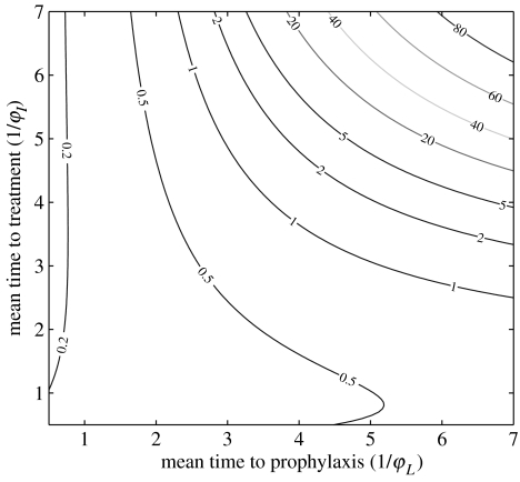
Although the model is useful for comparing treatment strategies, a strong warning is in order. The number of doses of antiviral treatment needed as predicted by the model is essentially proportional to the number of members of the population infected during the epidemic. This number is very sensitive to the number of infectives introduced initially. Introducing two infectives instead of one initially would multiply the number of members infected during the epidemic and the number of doses required by 1.4. This means that since the number of initial infectives cannot be known in advance, the model cannot predict with any degree of reliability the number of doses which would be required in an epidemic. This underscores the importance of early identification of infectives to minimize the number of initial infectives in the system. However, the relative effectiveness of different management strategies is not affected by this critical dependence. We may also estimate the number of cases of disease per 1000 members of the population as a function of the treatment parameters, and this is shown in figure 4 (as calculated from (11) in the electronic supplementary material but not including the index case).

Figure 4.

Total cases as a function of the treatment rates, for $\mathcal{R}$₀=1.5, with S₀=999 and I₀=1.

A scenario considered in Gani et al. (2005) is antiviral treatment of essentially all symptomatic infectives. We calculate that if $\mathcal{R}$₀=1.5 and antiviral treatment is applied only to symptomatic infectives, a rate φ_I=0.4 per day would be required to bring the control reproduction number $\mathcal{R}$_c down to 1 and avert an epidemic, as can be seen in figure 3.

Another application of the treatment model is to the common annual vaccination program to protect against the strain of influenza thought to be the most likely to invade. It has also been suggested (Balicer et al. 2005) that a possible response to an outbreak of a strain for which no specific vaccine has been developed as yet would be a program of treatment with a general antiviral as a stopgap until a specific vaccine can be produced. The model we have described can be applied to this limited drift situation as well, although the final size relation takes a more complicated form. With disease parameters as in Longini et al. (2004) and vaccination that reduces susceptibility by 70% of a fraction γ of the population before an epidemic and introduction of one infective into a total population of 1000 individuals, we obtain the results shown in table 1 for the number S_∞ of members untreated but uninfected during the epidemic, the number S_T∞ of members treated and uninfected during the epidemic and N_f, the number of cases of disease during the epidemic. They indicate the benefits in reducing influenza cases of pre-epidemic vaccination of even a small fraction of the population. The fraction of the population that must be vaccinated to bring the reproduction number down to 1 is 0.28, but as shown in table 1, a significant decrease in the number of cases of disease is achieved even if the reproduction number is not decreased to 1.

Table 1.

Fraction treated γ, untreated susceptibles S_∞, treated susceptibles S_T∞ and influenza cases N_f, with vaccination.

γ	S∞	ST∞	Nf
0	511	0	326
0.05	540	34	278
0.1	57	73	227
0.15	602	118	173
0.2	635	170	117
0.25	665	230	62
0.30	670	291	22

5. Conclusions

Compartmental models facilitate the analysis of sensitivity of the model to errors in measuring parameters or to changes in the control parameters. This is particularly valuable before the beginning of an epidemic when the values of some parameters are only guesses. For example, a sensitivity analysis of our model shows the importance of estimating the parameter p representing the fraction of latent members that will develop symptoms. This parameter is almost impossible to determine accurately, and it is taken to be 2/3 in Longini et al. (2004) and 1/2 in Ferguson et al. (2005). In view of the many uncertainties in estimating parameters for pandemic influenza, it is important to consider a large range of values, and the simplicity of calculation offered by a deterministic compartmental model lends itself to doing this as an initial step before more complicated models such as those of Ferguson et al. (2005) and Longini et al. (2005) are invoked. The calculations reported here involve nothing more complicated than the solution of a system of two transcendental equations.

Supplementary Material

1. The basic epidemic model 2. The treatment model

References

- Balicer R.D, Huerta M, Davidovitch N, Grotto I. Cost-benefit of stockpiling drugs for influenza pandemic. Emerg. Infect. Dis. 2005;11:1280–1282. doi: 10.3201/eid1108.041156. [DOI] [PMC free article] [PubMed] [Google Scholar]
- Brauer F. Some simple epidemic models. Math. Biosci. Eng. 2006;3:1–15. doi: 10.3934/mbe.2006.3.1. [DOI] [PubMed] [Google Scholar]
- Diekmann O, Heesterbeek J.A.P. Wiley; Chichester: 2000. Mathematical epidemiology of infectious diseases. [Google Scholar]
- Ferguson N.M, Cummings D.A.T, Cauchemez S, Fraser C, Riley S, Meeyai A, Iamsirithaworn S, Burke D.S. Strategies for containing an emerging influenza pandemic in Southeast Asia. Nature. 2005;437:209–214. doi: 10.1038/nature04017. doi:10.1038/nature04017 [DOI] [PubMed] [Google Scholar]
- Gani R, Hughes H, Griffin T, Medlock J, Leach S. Potential impact of antiviral use on hospitalizations during influenza pandemic. Emerg. Infect. Dis. 2005;11:1355–1362. doi: 10.3201/eid1109.041344. [DOI] [PMC free article] [PubMed] [Google Scholar]
- Gumel A, et al. Modelling strategies for controlling SARS outbreaks. Proc. R. Soc. B. 2004;271:2223–2232. doi: 10.1098/rspb.2004.2800. doi:10.1098/rspb.2004.2800 [DOI] [PMC free article] [PubMed] [Google Scholar]
- Longini I.M, Halloran M.E, Nizam A, Yang Y. Containing pandemic influenza with antiviral agents. Am. J. Epidemiol. 2004;159:623–633. doi: 10.1093/aje/kwh092. doi:10.1093/aje/kwh092 [DOI] [PubMed] [Google Scholar]
- Longini I.M, Nizam A, Xu S, Ungchusak K, Hanshaoworakul W, Cummings D.A.T, Halloran M.E. Containing pandemic influenza at the source. Science. 2005;309:1083–1087. doi: 10.1126/science.1115717. doi:10.1126/science.1115717 [DOI] [PubMed] [Google Scholar]
- van den Driessche P, Watmough J. Reproduction numbers and subthreshold endemic equilibria for compartmental models of disease transmission. Math. Biosci. 2002;180:29–48. doi: 10.1016/s0025-5564(02)00108-6. doi:10.1016/S0025-5564(02)00108-6 [DOI] [PubMed] [Google Scholar]
Associated Data
This section collects any data citations, data availability statements, or supplementary materials included in this article.
Supplementary Materials