Modelling in molecular biology: describing transcription regulatory networks at different scales

Abstract

Approaches to describe gene regulation networks can be categorized by increasing detail, as network parts lists, network topology models, network control logic models or dynamic models. We discuss the current state of the art for each of these approaches. We study the relationship between different topology models, and give examples how they can be used to infer functional annotations for genes of unknown function. We introduce a new simple way of describing dynamic models called finite state linear model (FSLM). We discuss the gap between the parts list and topology models on one hand, and network logic and dynamic models, on the other hand. The first two classes of models have reached a genome-wide scale, while for the other model classes high-throughput technologies are yet to make a major impact.

1. Introduction

(a) Problem statement

The results of genome sequencing and other high-throughput technologies have given us estimates of the complexity of molecular networks. There are tens of thousands of elements (e.g. genes) and at least as many connections between them, but the old question ‘How does a (simple) cell work?’ looks ever more difficult to answer. Moreover, what does it mean to understand a network consisting of tens of thousands of elements? Can a descriptive approach to biology ever provide an answer? How can we communicate results in an ever-increasing flood of details?

(b) Modelling molecular biology

One way of approaching these questions is by developing models to describe complex systems like gene networks. Such models (as models in general) are intentional simplifications of the reality. Leaving out some features allows one to concentrate on understanding particular properties of a system while ignoring others, assuming they are less important for the particular question in mind. Once we have developed a satisfactory model for particular aspects of a real world system, we can focus our study on the properties of the model instead of the real world system. This should allow us to make predictions about the real world system based on the properties of the model and subsequently test the predictions in experiments. If the predictions are correct the model is correct, if the predictions are wrong we have to question the model, investigate the differences and change the model accordingly. The change in the model reflects the increase in knowledge of how the real system works. If the model is rich enough to describe important aspects of the system that we are particularly interested in, we can claim that we have made a significant step towards the understanding of the real world system.

(c) Simulation and reverse engineering of gene networks

Simulations effectively mean using a model to generate data, which can then be compared to experiments, while reverse engineering refers to an approach where one starts from data and tries to design a model that fits the data (semi-) automatically using particular modelling methods. The model is, therefore, derived from data and is judged by the results of simulations compared to new experimental data. For example, one could use a gene expression data set to construct a particular gene network model (with a given model class) that is consistent with the data. Inconsistencies between simulated data generated using this model and new data, that has not been used to construct the model, indicate shortcomings of the model. These inconsistencies can be used to choose between alternative models, or to improve the model. However, simulations or reverse engineering is possible only if we have enough quantitative data describing the behaviour of the system.

(d) Dilemma of lacking data in times of high-throughput biology

The availability of large-scale data sets such as microarray gene expression and genomic localization data triggered the search for suitable approaches to model complex biological systems. However, currently it seems not feasible to simulate even relatively simple cells like baker's yeast or fission yeast accurately. Despite being two of the best-studied organisms the function of about one-third of all yeast genes is still unknown. And even for many of the better-known genes there is still not enough data available to exactly know all changes in concentration and activation patterns to simulate core processes that have been studied for decades, like the cell cycle. Models have been built to explore the fundamentals of the cell cycle for yeast (Tyson et al. 2002). However, these models describe only the behaviour of a few genes, while genome-wide gene expression studies (microarrays) show that hundreds of genes are changing their expression levels during the cell cycle (Spellman et al. 1998; Rustici et al. 2004). More recently significant improvements in the understanding of genome wide dynamics of the cell cycle have been made (de Lichtenberg et al. 2005), nevertheless we are not yet able to simulate the cell cycle quantitatively.

(e) Finite state linear model

To illustrate the points discussed above, let us introduce a ‘toy example’ for modelling gene regulatory networks, which we call the finite state linear model (FSLM). It has a control component based on discrete states (e.g. gene is ‘on’ or ‘off’), and an environment of substances changing their concentrations continuously. Time is continuous: the state of the network directly determines the concentration change rates, while the state is in turn affected by the concentrations themselves.

(i) Definition of the FSLM

Different classes of molecules, like mRNA or proteins, are not distinguished in the FSLM, they are all represented by substances. The FSLM comprises several such abstract substances, and three types of network elements: binding sites, control functions and substance generators (figure 1a). The binding sites in the FLSM correspond to DNA binding sites for transcription factors in the promoter regions of genes. A biological promoter corresponds to a control function connected to one or several binding sites in the FSLM. A combination of binding site(s), control function(s) and a substance generator in the FSLM corresponds to a biological gene (figure 1a). A gene network consists of several such genes, which influence each other via the substances they produce (figures 2 and 3). Here we will briefly describe the simpler binary version of the FSLM, which allows only two possible states for the binding sites and substance generators. A description of the multilevel model, where this restriction is lifted, and a more mathematically thorough definition can be found in Brazma & Schlitt (2003).

Figure 1.

(a) The building blocks of the finite state linear model: binding sites are represented by triangles, control functions by boxes and substance generators by diamonds. Dotted lines represent cases where the discrete output of one element is the input for another element. (b, c) Switching behaviour of the binding sites. The curve (b) is typical for processes with hysteresis characteristics of a system that does not instantly follow the forces applied to it, but reacts slowly, or does not return completely to its original state: that is, systems whose states depend on their immediate history. The threshold for switching the states of the binding sites in FSLM is state-dependent and results in a similar curve (c). [c] concentration of substance binding to binding site j; asso_j, disso_j, association and dissociation constants for binding site j; u, binding site not occupied; o, binding site occupied.

Figure 2.

Example for the dynamics of a simple network: (a) in this negative feedback loop the substance generator produces a substance which acts as a repressor of its own control function. (b) Environment change graph recording the changes in repressor concentration during time. From the initial concentration the repressor accumulates with rate r⁺ until the association constant of the binding site b_rep is reached at time t₁. Then the substance generator is switched off and the repressor degrades with rate r⁻ until the dissociation constant is reached at time t_2. The substance generator then produces the repressor until the association constant is reached again (¬ means Boolean ‘not’).

(ii) The binary version of the FSLM

In the environment there are n different substances, each corresponding to a particular substance generator. These substances can bind to binding sites. Each binding site can be bound by one particular substance. A binding site can be in one of two states, bound or unbound. The binding of a substance to a binding site b_j depends on the association constant asso_j and the dissociation constant disso_j of the binding site (0<disso_j<asso_j). If the concentration of the binding substance is equal to, or greater than, its association constant then the binding site is bound. If the substance concentration falls below the dissociation constant then the binding site is not bound by the substance anymore and it switches to the unbound state. The biochemical equivalents of the association and dissociation constants in FSLM are affinity constants. The difference between the association constant asso_j corresponding dissociation constant disso_j leads to hysteresis characteristics (figure 1b) for the switching between the states of a binding site (see for example Tyson & Novak 2001). The concentration threshold for the switch between the states of the binding site depends on the state of the binding site itself. Using discrete states to represent the binding sites means we approximate the binding equilibrium with a simpler step function.

The states of a set of binding sites comprise the input vector of a control function F. This control function is a Boolean function. Depending on the input state vector the control function computes an output state (on or off). A substance generator S changes the concentration of a substance in time in a linear fashion. The concentration can either increase with rate r⁺ or decrease with rate r⁻ (r⁻<0<r⁺), corresponding to substance production and degradation, respectively. The output state of a control function determines the activity of a substance generator, i.e. whether the concentration of a particular substance is increasing or decreasing.

(iii) Dynamics of the FSLM

The dynamics of the FSLM can be illustrated by modelling a negative feedback loop involving a single gene (figure 2). At the start, the substance concentration is low, the binding site is unbound, the substance generator is active and, therefore, the substance is produced with rate r⁺. Its concentration increases until it reaches the association constant of the binding site. The binding site switches to the bound state, which in turn leads to the inactivation of the substance generator, and the substance concentration decreases with rate r⁻ until it reaches the dissociation constant of the binding site. Consequently, the binding site switches to the unbound state, the substance is generated again, its concentration increases and the process repeats itself. Figure 3 shows the behaviour of a gene network consisting of two genes, demonstrating that a very simple network of just two genes can exhibit a non-trivial behaviour.

Figure 3.

A network consisting of two genes and four binding sites. (a) The control functions of both genes have two inputs each. One input is from a binding site for its own substance, thus each gene is autoregulated by a negative feedback loop. Gene 1 has an additional negative feedback on gene 2, while gene 2 has an additional positive feedback on gene 1. (b) Result of the simulation of this network in FSLM. a1 association constant of binding site 1, d1 is the corresponding dissociation constant; a2, d2, a3, d3, a4, d4 correspondingly; ¬ Boolean ‘not’, & Boolean ‘and’.

FSLM can be used to build complex models for instance to simulate the life cycle of phage λ (figure 4). Our simulations of phage λ show that the FSLM model allows two different kinds of behaviours, which correspond to lytic or lysogenic behaviour.

Figure 4.

Description of phage λ using the elements of FSLM. Phage λ is a bacteriovirus that can infect Escherichia coli cells (Ptashne 1992). Depending on the growth conditions it either integrates into the host genome and stays dormant (lysogenic), or causes production of new phage particles and lysis of the host cell, to allow infecting neighbouring cells. The decision for one or the other alternative (lysis versus lysogeny) is made by the so-called lambda switch, which is based on competitive binding of two transcription factors to overlapping regions in the genome of phage λ. If the repressor is bound, the phage stays dormant, if the repressor is degraded and the activator can bind, new virus particles are being made. In the FSLM model for phage λ the substance generators highlighted in grey produce substances, which bind to binding sites on the left (the connections have been omitted to improve the readability of the figure). The promoters P_L1, P_L2, P_R1 and P_R2 are used to model the behaviour of the λ terminator sites t_L1, t_L2, t_R1 and t_R2. The substance generators connected to them are only active if n is bound to the respective binding sites. The substance ‘Struc’ represents the structural proteins of the phage particles. The shaded grey boxes indicate the number of different states that the corresponding control functions can have. A simulation of phage λ using this model leads to lysogenic behaviour or lytic behaviour. In the lysogenic mode the initially active genes are inactivated, and the substance concentrations decrease rapidly, only the repressor cI is produced. The fluctuations of the cI concentration are due to the negative feedback loop involving the binding site O_R3. In the lytic mode, cI and cII are not produced, but the other substance generators are active. The concentrations of int, N and Q increase infinitely because of the lack of a negative feedback control. The inset describes the effect of the stress response of the host cell using elements not yet implemented in the FSLM simulator. For a more detailed description of the model see Brazma & Schlitt (2003). Summary of λ gene functions: cI, λ repressor; cII, cIII, establishment of lysogeny; N, Q, anti-terminators for early and delayed early genes; O, P, origin recognition in DNA replication; int, integration and excision of phage DNA; xis, excision of phage DNA; R, S, host lysis; O_R, operator sites; P, promoters; T, terminators (see Ptashne 1992).

(iv) What do we need to describe a biological system with FSLM?

These very simple examples of gene networks illustrate the modelling process of biological systems in a nutshell. However, can this be applied to networks consisting of thousands of genes? To begin with, we need to have a list of the parts involved in the system to be modelled; next we need to know the topology of the network: which substances, binding sites and control functions are connected to each other. We also need to know the control functions, and we need to know the appropriate binding constants and rate constants.

In our example, the information required about the biological system is relatively trivial, but when the network size increases, the lack of detailed biological information becomes a major bottleneck for its modelling. So, what can we do if we do not have sufficient information to build large-scale dynamic models? Instead of building the full dynamic model, we can start with compiling the parts lists, next describing the connections (the topology), then the control logics and eventually the dynamics (Schlitt & Brazma 2005).

2. Classification of existing modelling approaches—four levels of hierarchical description

(a) Parts lists

Simple parts lists (of genes, transcription factors, promoters, binding sites, …) are useful means for assessing the network complexity and for comparing different organisms. Such parts lists are results of genome sequencing and annotation projects, and although gene identification and annotation are not a trivial exercise, parts list give a good first impression of the complexity of an organism.

For example, we can compare the parts lists for two very different yeasts—Saccharomyces cerevisiae and Schizosaccharomyces pombe (table 1). Note that although they have roughly the same number of genes, evolutionary they are as far from each other as for instance from human. Despite similar genome size there are obvious differences in genome organization (Goffeau et al. 1996; Wood et al. 2002). The intergenic sequences in S. pombe are on average larger than in S. cerevisiae, and about 43% of all genes in S. pombe contain introns compared to only 5% in S. cerevisiae. Introns allow alternative splicing; therefore the complexity of the proteome of S. pombe might be higher than that of S. cerevisiae. Sequence data in combination with functional information, based on genome annotation or expression data, allows identifying conserved sequences in putative promoter regions which might be potential binding sites for transcription factors. A striking result of the cell cycle study in S. pombe is to find that the presence or absence of consensus binding sites in the promoter regions corresponds to the cyclic expression pattern of the genes (Rustici et al. 2004). Genes with a peak expression at similar cell cycle stage share similar sets of consensus binding sites. Although facing large error margins, we can get a first impression of the complexity of the gene expression in different organisms by comparing their repertoire and location of consensus binding sites for transcription factors.

Table 1.

Comparison of some genomic features of Schizosaccharomyces pombe and Saccharomyces cerevisiae.

	S. pombe	S. cerevisiae
genome size	∼14 Mb	∼13 Mb
number of chromosomes	3	16
number of predicted genes	∼4900	∼5800
number of predicted introns	∼4700	∼300
proportion of protein-coding sequences of genome	60%	70%

However, the computational identification of consensus binding sites does not automatically lead to the identification of the binding factors.

(b) Topological network models

Large screens using chromatin immunoprecipitation in conjunction with genomic microarrays (ChIP-on-chip technology) have been used to identify the genomic localization of transcription factors (Lee et al. 2002). Once we know the transcription factor binding sites, we can describe the gene transcription regulatory networks using graph-based methods. Such topological models—graphs describing the connections between the parts—have been used for various biological data sets ranging from protein–protein interactions networks to coexpression networks. In general, data sets used for topological models have one important limitation. While hundreds of organisms have been fully sequenced and many genes are identified relatively reliably, the data sets underlying most topological models are much less complete. For example, only a fraction of all protein–protein interactions in yeast have been tested, for various reasons: one needs to perform 6000×6000/2 yeast-2-hybrid experiments plus controls, and not all proteins are likely to be expressed as desired. This problem is made even worse by the nature of the data; most large-scale experiments show high noise levels. And whereas the genome sequence is independent of particular growth conditions and might even be conserved in fossils, data like protein–protein interactions and transcription factor localizations are condition-dependent. Therefore, we have to work with incomplete data for a limited set of conditions.

(i) Comparison of yeast networks

In the following, we would like to illustrate the knowledge we can obtain from of studying the network topology by giving an example of how to use the topology to compare and combine information from various high-throughput data sets for gene networks in S. cerevisiae.

If we want to understand the gene regulation network, all types of information have to be integrated and analysed in combination. In particular, we combine three different data sets using a graph-based approach, two are based on experimental data: chromatin immunoprecipitation experiments for transcription factors (ChIP network; Lee et al. 2002) and microarray experiments on single gene deletion mutants (mutant network; Hughes et al. 2000); the third is based on the computational analysis of transcription factor binding sites (in-silico network; Pilpel et al. 2001). In the graph representation of the data, the nodes correspond to genes and an arc connects two genes, if the first gene has a particular (asymmetric) relationship to the second one (Schlitt & Brazma 2002). Thus in the ChIP network, an arc A→B means that the gene A codes for a transcription factor that binds to the promoter of gene B, in the in-silico network it means that the predicted binding site of A has a match in the promoter of B, while in the mutant network it means that the mutation of A will change the expression level of B (Schlitt et al. 2003).

We call genes with outgoing connections source genes; for each source gene we define the target set as the set of all genes with incoming connections from that particular source gene. These networks differ in size, the in-silico network has the smallest number of source genes, but the ChIP network has the smallest number of target genes (table 2). This discrepancy might be due to over prediction of binding sites in case of the in-silico network, but it is likely that in the ChIP network not all potential binding sites are identified, because only a fraction of sites might have been occupied under the particular experimental conditions applied. Note that all three networks depend on various thresholds applied to the continuous experimental data. Since the criteria used to choose these thresholds are rather subjective, only trends in the properties of these networks are meaningful, rather than the exact sizes. All three networks consist of one major connected component; almost all genes are part of it. The degree distributions for the mutant network and the ChIP network resemble roughly a power-law, whereas in the in-silico network nodes with a very small number of connections are underrepresented (figure 5).

Table 2.

Comparison of three different networks for S. cerevisiae.

	ChIP network	in-silico network	mutant network
source genes	106	38	170
genes	2363	5581	4046
connections	4358	23 446	12 205
size of largest component	2403	5583	4095
size of second largest component	11	—	2

Figure 5.

Log–log plot of the node connectivity in different topological networks. The genes with the highest connectivity are ABF1 in the ChIP-network, SWI5 in the in-silico-network, and TUP1 in the mutant network.

Comparison of yeast networks

The intersection of the in-silico network with the mutant network and the ChIP network is sparse, 34 connections can be found in all three of them. In protein–protein interaction networks, too, a relatively small number of interactions are reported by several experiments, and these interactions are more reliable than most of the data (von Mering et al. 2002). The same is true for the networks examined here: the genes connected in all three networks are functionally related. Among the 40 genes shared by all networks is STE12, which encodes a transcription factor and is part of the mating response, as are the five genes connected to it (figure 6). A guilt-by-association approach based on the network connectivity can, therefore, be used to identify possible biological functions for uncharacterized genes. See for example connections from SWI5, a transcription factor that controls cell cycle-specific transcription of SIC1 and YKL185W (ASH1); all genes connected to SWI5 are annotated to be involved in cell growth and maintenance (SIC1, CHS1, CCW6 (PIR1), YKL185W (ASH1)), or lack a biological process annotation in SGD (YGR086C (PIL1), YLR049C, YDR055W (PST1), YLR194C, YPL158C). Therefore, we can hypothesize that the latter genes are also involved in maintenance/cell growth related processes under the control of SWI5p. This hypothesis is in agreement with several previous publications (Spellman et al. 1998; Jung & Levin 1999; Doolin et al. 2001).

Figure 6.

Intersection of the in-silico network with the mutant network and the ChIP network. Only 34 connections (red) can be found in all three of them. In addition this figure shows all connections between SWI4, SWI6 and MBP1 present in two of the networks (green). Box-shaped nodes indicate all genes with unknown function. SWI4 interacts with either SWI6 to form the SBF complex or with MBP1 to form the MBF complex (Ho et al. 1997). Genes connected to SWI4 and SWI6 (highlighted green) are likely to interact with SBF, genes connected to SWI4 and MBP1 (highlighted in blue) are likely to interact with MBF. Some genes might interact with both MBF and SBF (highlighted in yellow). Genes connected to MBP1 and SWI6 are highlighted in red.

Neighbourhood comparison

To combine these networks in a meaningful way we use statistical methods to compare target sets of all source genes (Schlitt et al. 2003). We ask for which source genes studied by two different techniques the target sets overlap more than expected by chance (figure 7). The target sets in the ChIP network match well with the target sets in the in-silico network for 14 out of 26 transcription factors examined by both techniques (figure 8). The effect of 2 (out of 7) transcription factor deletions on the expression pattern is in correspondence with their genomic localization according to the in-silico network—similar results were obtained by Palin et al. (2002). The ChIP network and the mutant network have 14 transcription factors in common. Only the genomic localization (ChIP network) of the 6 transcription factors MBP1p, ARG80p, YAP1p, SWI5p, STE12p and GCN4p corresponds well with the changes in gene expression (mutant network) observed in the respective deletion mutants (figure 8).

Figure 7.

Illustration of the target set comparison. (a) In the ChIP network transcription factors are connected to their target genes (regulation set); in the mutant network the deleted genes are linked to all genes with differential expression in this particular mutant background (effectual set). (b) Some transcription factors are present in both networks (ChIP and mutant network); we can, therefore, compare the genomic localization (regulation set) with the expression changes in the mutant cell (effectual set).

Figure 8.

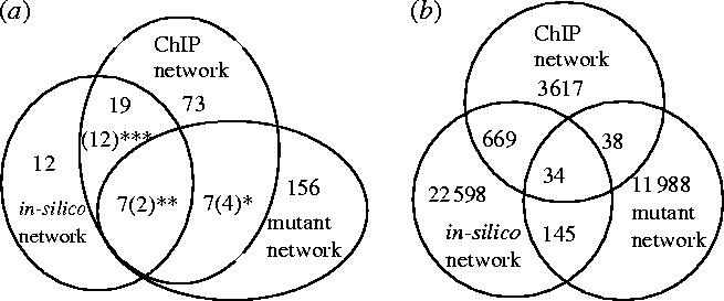
The Venn diagrams illustrate the overlap between the in-silico, the mutant and the ChIP network. (a) Number of source genes shared by several networks, in brackets number of source genes with significantly similar target sets in the different networks (^*SWI5, YAP1, MBP1, ARG80, ^**GCN4, STE12, ^***ABF1, BAS1, GAL4, HAP4, LEU3, MBP1, MCM1, RAP1, REB1, SWI6, YAP1, ZAP1). (b) Number of connections shared by the networks.

Indirect effects

Note that we do not expect perfect coincidence among the three networks. For instance, the mutant network can be expected to have additional relationships, because regulatory or signalling cascades link some genes. The physical interaction networks, on the other hand, do not necessarily tell us anything about the effect of connected genes, except that there is evidence that the first gene encodes a transcription factor which binds to the putative promoter of the second gene.

As described above for some transcription factors we found a correspondence between the localization of a transcription factor and the set of genes affected by its deletion. We analysed how often the effects seen in the mutant network can be explained by indirect connections via one additional factor in the ChIP network (figure 9a). Some subnetworks resemble the single input motif (figure 9b) described by Lee et al. (2002) and Milo et al. (2002), with additional connections from the mutant network. For instance, some of effects of the deletion of GLN3, involved in nitrogen catabolite repression (NCR)-sensitive transcription regulation, may be due to indirect effects via GCN4 in the Δgln3 mutant (figure 9c); and the effects of deleting RTG1 on HIS4, ADE3, ADE4, ADE13 and ADE17 may be due to indirect effects via BAS1 (figure 9d). In a similar fashion, the effect of the YAP1 deletion on ENB1 (YOL158C) may be due to indirect effects via YAP6 in the Δyap1 mutant (figure 9e). At the same time the deletion of YAP1 may influence the expression level of FET4 via the transcription factors YAP6, ROX1, or both (figure 9e). However, these regulatory interactions may be intriguingly interlinked, as is the case for the cell cycle regulators MBP1, SWI4, SWI6 and NDD1 (figure 9f). This subnetwork seems to consist of a combination of several single input motifs.

Figure 9.

(a) The deletion of transcription factor X may affect gene Z, because X controls the expression of Z (direct effect). It is also possible that the deletion of transcription factor X affects gene Z indirectly, via a direct effect on transcription factor Y. (b) The single input motif as defined by Shen-Orr et al. for a Escherichia coli network and Lee et al. for the ChIP network. (c–f) All cases where a single connection in the mutant network corresponds to two connections in the ChIP network. (c) and (d) resemble the single input motif, with an additional top layer of regulation, whereas (e) and (f) correspond to more complex combinations of network motifs. dashed green, connections in the mutant network; solid red, connections in the ChIP network.

These examples illustrate that graph representation is a useful tool to examine general properties of large functional genomics data sets. Not only can it be used to examine the properties of single data sets, for example in the form of protein–protein interaction networks, but it is also useful to compare and integrate various large-scale data sets. It can be used to distinguish between noise and signals in these data sets, and it can also be used to derive functional predictions, which can be evaluated by wet lab experiments (Schlitt et al. 2003; Lee et al. 2004; Kemmeren et al. 2005).

(c) Control logics: analysing the rules behind the network

Once we know the topology of the network, the next step is to address the rules of interaction between the different elements in the network. For instance, if a promoter consists of only one binding site for a transcription factor, we need to know whether this factor acts as an activator or as a repressor. If more than one transcription factor binds to a promoter, we need to know not only what each factor does, but also how these factors interact (figure 10). In FSLM the control logics corresponds to the rules expressed by the control functions. Biological studies show that at least some promoters consist of elements comprising Boolean behaviour (Louis & Becskei 2002). The group of Davidson analysed the Endo16 promoter of sea urchin in detail and were able to express the interactions between various functional elements in the promoter by a set of rules which allow predicting the gene activity. A large part of those rules are Boolean functions, such as AND, OR, XOR, NOT (Yuh et al. 1998). Later the same group extended their work to describe the interactions between a large set of genes in sea urchin (Davidson et al. 2002).

Figure 10.

Example for network logics: genes A, B and C control the activity of gene D; D is active if A and B are bound, but not C; (b) shows the FSLM representation for such a promoter.

In a different approach, instead of using discrete states to represent the gene activity and Boolean functions to describe the logics, we could use continuous values g to represent the gene activity, and weights w to represent the interaction between genes. Thus, the activity of gene i can be calculated as the weighted sum of the activity of all n genes

$$g_i=\sum _j^n{w}_{ij}{g}_j.$$

There are situations where neither Boolean rules nor linear functions are powerful enough to express the control logics: transcription factors might bind competitively; if one factor is bound the other one is excluded, as is the case for example in the lambda switch between lysis and lysogeny. In other cases, transcription factors have to form homodimers or heterodimers to be fully functional. It might be that factors have to bind sequentially or act synergistically. In these situations it might be necessary to use mathematical functions that allow more flexibility than Boolean functions to express the control functions correctly. It remains an open question what the minimum repertoire of logic functions is to describe all these processes.

A powerful approach to test our understanding gene regulatory networks is to modify existing networks or to build new networks from scratch in an approach called synthetic biology. Several small systems have been designed and tested in vivo in Escherichia coli, yeast and other organisms, see for example work by Becskei & Serrano (2000), Gardner et al. (2000), Kobayashi et al. (2004), and the reviews by Ball (2004) and Kaern et al. (2003).

Once we know the parts list of a network, its topology and the control logics, we can try to expand the model to capture dynamic changes during time.

(d) Dynamics: how does it all work in real time?

(i) Dynamic models

Various dynamic models for gene regulatory networks have been proposed and studied. In general, these models fall into three categories: Boolean network-based models (Liang et al. 1998; Szallasi & Liang 1998; Akutsu et al. 1999), dynamic systems described by differential or difference equations (Chen et al. 1999; D'Haeseleer et al. 1999; Holter et al. 2001; Tyson et al. 2002) and hybrid models (Thieffry et al. 1993; Mendoza et al. 1999; Akutsu et al. 2000; Smolen et al. 2000b). They can be subclassified using a classification suggested by Greller & Somogyi (2002):

Dichotomies for framing our thinking on how to best represent a particular biological network problem include the following distinguishing attributes: quantitative versus qualitative measurements; logical versus ordinal variables (e.g. Boolean versus abundances); deterministic versus probabilistic state transitions (e.g. differential equations versus hidden Markov); deterministic versus statistical overall system description (e.g. vector field versus Bayesian belief network probability distributions); continuous versus discrete state (e.g. continuous intensities or concentrations versus low, medium and high); nonlinear versus linear elementary interactions and state update rules (e.g. multiplicatives, sigmoids or non-monitonics versus linear ramps); high-dimensional versus low-dimensional (e.g. ≫100 s of variables versus ≪100 variables); stochasticity present and profound versus absent or present as nuisance noise (e.g. probabilistic state transitions versus small amplitude errors); measurement error substantially corrupting and obfuscating versus negligible distortion.

Each of these models has its advantages and drawbacks, we will discuss some of them briefly here.

(ii) Boolean networks—state spaces and attractors

Already at the end of the 1960s Stuart Kauffman studied Boolean networks as a model for gene regulatory networks (Kauffman 1969). Boolean networks are based on the assumption that binary on/off switches functioning in discrete time-steps can describe important aspects of gene regulation. In synchronous Boolean network models, one of the simplest dynamic models, all genes switch states simultaneously (figure 11). We can introduce the concept of the state of the network defined as an n-tuple of 0s and 1s describing which genes in the network are (or are not) expressed at a particular moment (figure 11b). As time progresses, the network navigates through the ‘state space’, switching from one state to another, as shown in figure 11d. For a network of n genes, in total there are 2ⁿ different states. We can follow the succession of states with time and thus identify attractors: these are states or series of states that once reached will not be left anymore. The small example network in figure 11 has two attractors: one attractor is a single state (0, 0, 1), and the second attractor consists of two alternating states (1, 0, 1) and (0, 1, 0). Kauffman (2002) hypothesized that attractors correspond to particular cell types, and based on different assumptions about the network (e.g. the average number of connections per gene and particular properties of the control logic) estimated the number of cell types which correspond well to the observations.

Figure 11.

Example for a small Boolean network consisting of three genes X, Y and Z. There are different ways for representing the network: (a) as a graph, (b) Boolean rules for state transitions, (c) a complete table of all possible states before and after transition, or (d) as a graph representing the state transitions.

Boolean models offer only a rather crude representation of real world gene networks. For example, even if we generalize these models to more than two discrete states they cannot describe continuous changes in the cell.

(iii) Difference and differential equation models—dilemma between oversimplification and sensitivity to many parameters

Continuous changes can be described using difference equations or differential equations (Chen et al. 1999; Hatzimanikatis 1999; von Dassow et al. 2000; Maki et al. 2001; Wahde & Hertz 2001).

The basic difference equation model is of the form

$$X_i(t+\mathrm{\Delta }t)=\sum _j{W}_{ij}{X}_j(t),$$

where X_i(t+Δt) is the expression level of gene i at time t+Δt, and W_ij indicates how much the level of gene j influences gene i. For each gene, one can add extra terms indicating the influence of additional substances, for instance drugs, and a constant bias term to capture the activation level of the gene in the absence of any other regulatory inputs. The formula then becomes

$$X_i(t+\mathrm{\Delta }t)=\sum _j{W}_{ij}{X}_j(t)+K_i{D}_i(t)+C_i+T_i,$$

where D_i(t) is the concentration of drug i at time t, K_i is the influence of the drug i on gene i, C_i is a constant bias factor for each gene and T_i indicates the difference in bias between different tissues (D'Haeseleer et al. 1999).

Differential equation models are similar to difference equation models, but follow concentration changes continuously, modelling the time-difference between two time-steps in infinitely small increases.

Dynamic networks models have been reviewed intensively (Smolen et al. 2000a; Brazhnik et al. 2002; de Jong 2002; van Someren et al. 2002). One of the largest transcription network models using differential equations we are aware of is a model for early development of Drosophila by von Dassow et al. (2000) (5 genes, 13 differential equations, 48 parameters).

(iv) Reverse engineering

The methods chosen for reverse engineering depend crucially on the kind of modelling technique used. Dynamic models contain many parameters, and detailed experimental data is required to work out the parameters. Quantitative models are obviously more demanding that qualitative models. There are approaches to perform reverse engineering for dynamic models. Tegner et al. (2003) proposed an approach for the reverse engineering of dynamic gene networks based on integrating genetic perturbations. They identified ‘[…] the network topology by analysing the steady-state changes in gene expression resulting from the systematic perturbation of a particular node in the network.’ (Tegner et al. 2003). However, they only apply their approach to simulated data and to a comparatively small biological system consisting of only five genes.

(v) Hybrid models

Models based on differential equations cannot easily describe the discrete aspects of gene regulation, such as the binding of a transcription factor to the DNA, which is essentially an on/off event. It is not straightforward to describe non-additive logics in gene regulation (for instance, competitive events).

Models trying to combine the discrete and continuous components have therefore been proposed, for instance (Mendoza et al. 1999; Akutsu et al. 2000; Smolen et al. 2000b). Thieffry & Thomas (1998) describe a combined model for the qualitative description of gene regulatory networks (Thomas 1991). They introduce a notion of gene state and image, the last effectively representing the substance produced by the respective gene. There is a time delay between the change of the gene state and the change of the image state. By introducing several levels of gene activity and thresholds for switching the gene states they go beyond binary models, but they do not make continuous changes possible.

The FSLM we introduced in the beginning combines advantages of Boolean networks such as simplicity and low-computational cost, with the advantages of continuous models, such as continuous representation of concentrations and time in a simple and structured way.

3. Outlook

How far are we from being able to build realistic cell models? As the result of genome projects we are now building gene network parts lists on genome scale, though we do not know how many important categories in these parts lists are missing (e.g. different types of micro RNAs). Mechanisms like RNA interference, regulated degradation of mRNAs and proteins, chemical modifications of key molecules and others might play a larger role than anticipated in current models, other processes might still be unknown. High-throughput technologies are providing us with some information on genome scale for model organisms such as yeasts. Then again, important processes, such as spatial effects, are still poorly understood. But this is where the impact of high-throughput technologies largely stops, though there have been attempts to use high-throughput datasets to study the combinatorial control logics (Wang et al. 2005). As far as dynamic models are concerned the existing models typically cover only few genes. The question ‘Is real time simulation on genome scale possible at all?’ is still open. Probably the answer largely depends on the modularity properties of the real world gene networks, and their robustness (stability against changes of various network parameters and initial conditions). If the networks are modular, it might be possible to build genome scale networks as sets of smaller modules. If the exact values of parameters and molecular concentrations are not crucial, it might be possible to simulate the cell in terms of some more abstract states than substance concentrations. In any case, finding the right language for describing the models is a prerequisite for success.

References

- Akutsu T, Miyano S, Kuhara S. Identification of genetic networks from a small number of gene expression patterns under the Boolean network model. Pac. Symp. Biocomput. 1999:17–28. doi: 10.1142/9789814447300_0003. [DOI] [PubMed] [Google Scholar]
- Akutsu T, Miyano S, Kuhara S. Algorithms for inferring qualitative models of biological networks. Pac. Symp. Biocomput. 2000:293–304. doi: 10.1142/9789814447331_0028. [DOI] [PubMed] [Google Scholar]
- Ball P. Synthetic biology: starting from scratch. Nature. 2004;431:624–626. doi: 10.1038/431624a. 10.1038/431624a [DOI] [PubMed] [Google Scholar]
- Becskei A, Serrano L. Engineering stability in gene networks by autoregulation. Nature. 2000;405:590–593. doi: 10.1038/35014651. 10.1038/35014651 [DOI] [PubMed] [Google Scholar]
- Brazhnik P, de la Fuente A, Mendes P. Gene networks: how to put the function in genomics. Trends Biotechnol. 2002;20:467–472. doi: 10.1016/s0167-7799(02)02053-x. 10.1016/S0167-7799(02)02053-X [DOI] [PubMed] [Google Scholar]
- Brazma A, Schlitt T. Reverse engineering of gene regulatory networks: a finite state linear model. Genome Biol. 2003;4:P5. 10.1186/gb-2003-4-6-p5 [Google Scholar]
- Chen T, He H.L, Church G.M. Modeling gene expression with differential equations. Pac. Symp. Biocomput. 1999:29–40. [PubMed] [Google Scholar]
- Davidson E.H, et al. A genomic regulatory network for development. Science. 2002;295:1669–1678. doi: 10.1126/science.1069883. 10.1126/science.1069883 [DOI] [PubMed] [Google Scholar]
- de Jong H. Modeling and simulation of genetic regulatory systems: a literature review. J. Comput. Biol. 2002;9:67–103. doi: 10.1089/10665270252833208. 10.1089/10665270252833208 [DOI] [PubMed] [Google Scholar]
- de Lichtenberg U, Jensen L.J, Brunak S, Bork P. Dynamic complex formation during the yeast cell cycle. Science. 2005;307:724–727. doi: 10.1126/science.1105103. 10.1126/science.1105103 [DOI] [PubMed] [Google Scholar]
- D'Haeseleer P, Wen X, Fuhrman S, Somogyi R. Linear modeling of mRNA expression levels during CNS development and injury. Pac. Symp. Biocomput. 1999:41–52. doi: 10.1142/9789814447300_0005. [DOI] [PubMed] [Google Scholar]
- Doolin M.T, Johnson A.L, Johnston L.H, Butler G. Overlapping and distinct roles of the duplicated yeast transcription factors Ace2p and Swi5p. Mol. Microbiol. 2001;40:422–432. doi: 10.1046/j.1365-2958.2001.02388.x. 10.1046/j.1365-2958.2001.02388.x [DOI] [PubMed] [Google Scholar]
- Gardner T.S, Cantor C.R, Collins J.J. Construction of a genetic toggle switch in Escherichia coli. Nature. 2000;403:339–342. doi: 10.1038/35002131. 10.1038/35002131 [DOI] [PubMed] [Google Scholar]
- Goffeau A, et al. Life with 6000 genes. Science. 1996;274:563–567. doi: 10.1126/science.274.5287.546. 10.1126/science.274.5287.546 [DOI] [PubMed] [Google Scholar]
- Greller L.D, Somogyi R. Reverse engineers map the molecular switching yards. Trends Biotechnol. 2002;20:445–447. doi: 10.1016/s0167-7799(02)02051-6. 10.1016/S0167-7799(02)02051-6 [DOI] [PubMed] [Google Scholar]
- Hatzimanikatis V. Nonlinear metabolic control analysis. Metab. Eng. 1999;1:75–87. doi: 10.1006/mben.1998.0108. 10.1006/mben.1998.0108 [DOI] [PubMed] [Google Scholar]
- Ho Y, Mason S, Kobayashi R, Hoekstra M, Andrews B. Role of the casein kinase I isoform, Hrr25, and the cell cycle-regulatory transcription factor, SBF, in the transcriptional response to DNA damage in Saccharomyces cerevisiae. Proc. Natl Acad. Sci. USA. 1997;94:581–586. doi: 10.1073/pnas.94.2.581. 10.1073/pnas.94.2.581 [DOI] [PMC free article] [PubMed] [Google Scholar]
- Holter N.S, Maritan A, Cieplak M, Fedoroff N.V, Banavar J.R. Dynamic modeling of gene expression data. Proc. Natl Acad. Sci. USA. 2001;98:1693–1698. doi: 10.1073/pnas.98.4.1693. 10.1073/pnas.98.4.1693 [DOI] [PMC free article] [PubMed] [Google Scholar]
- Hughes T.R, et al. Functional discovery via a compendium of expression profiles. Cell. 2000;102:109–126. doi: 10.1016/s0092-8674(00)00015-5. 10.1016/S0092-8674(00)00015-5 [DOI] [PubMed] [Google Scholar]
- Jung U.S, Levin D.E. Genome-wide analysis of gene expression regulated by the yeast cell wall integrity signalling pathway. Mol. Microbiol. 1999;34:1049–1057. doi: 10.1046/j.1365-2958.1999.01667.x. 10.1046/j.1365-2958.1999.01667.x [DOI] [PubMed] [Google Scholar]
- Kaern M, Blake W.J, Collins J.J. The engineering of gene regulatory networks. Annu. Rev. Biomed. Eng. 2003;5:179–206. doi: 10.1146/annurev.bioeng.5.040202.121553. 10.1146/annurev.bioeng.5.040202.121553 [DOI] [PubMed] [Google Scholar]
- Kauffman S. Homeostasis and differentiation in random genetic control networks. Nature. 1969;224:177–178. doi: 10.1038/224177a0. [DOI] [PubMed] [Google Scholar]
- Kauffman S.A. Investigations. Oxford University Press Inc; USA: 2002. [Google Scholar]
- Kemmeren P, Kockelkorn T.T, Bijma T, Donders R, Holstege F.C. Predicting gene function through systematic analysis and quality assessment of high-throughput data. Bioinformatics. 2005;21:1644–1652. doi: 10.1093/bioinformatics/bti103. 10.1093/bioinformatics/bti103 [DOI] [PubMed] [Google Scholar]
- Kobayashi H, Kaern M, Araki M, Chung K, Gardner T.S, Cantor C.R, Collins J.J. Programmable cells: interfacing natural and engineered gene networks. Proc. Natl Acad. Sci. USA. 2004;101:8414–8419. doi: 10.1073/pnas.0402940101. 10.1073/pnas.0402940101 [DOI] [PMC free article] [PubMed] [Google Scholar]
- Lee T.I, et al. Transcriptional regulatory networks in Saccharomyces cerevisiae. Science. 2002;298:799–804. doi: 10.1126/science.1075090. 10.1126/science.1075090 [DOI] [PubMed] [Google Scholar]
- Lee I, Date S.V, Adai A.T, Marcotte E.M. A probabilistic functional network of yeast genes. Science. 2004;306:1555–1558. doi: 10.1126/science.1099511. 10.1126/science.1099511 [DOI] [PubMed] [Google Scholar]
- Liang S, Fuhrman S, Somogyi R. Reveal, a general reverse engineering algorithm for inference of genetic network architectures. Pac. Symp. Biocomput. 1998:18–29. [PubMed] [Google Scholar]
- Louis M, Becskei A. Binary and graded responses in gene networks. Sci. STKE. 2002;2002:E33. doi: 10.1126/stke.2002.143.pe33. [DOI] [PubMed] [Google Scholar]
- Maki Y, Tominaga D, Okamoto M, Watanabe S, Eguchi Y. Development of a system for the inference of large scale genetic networks. Pac. Symp. Biocomput. 2001:446–458. doi: 10.1142/9789814447362_0044. [DOI] [PubMed] [Google Scholar]
- Mendoza L, Thieffry D, Alvarez-Buylla E.R. Genetic control of flower morphogenesis in Arabidopsis thaliana: a logical analysis. Bioinformatics. 1999;15:593–606. doi: 10.1093/bioinformatics/15.7.593. 10.1093/bioinformatics/15.7.593 [DOI] [PubMed] [Google Scholar]
- Milo R, Shen-Orr S, Itzkovitz S, Kashtan N, Chklovskii D, Alon U. Network motifs: simple building blocks of complex networks. Science. 2002;298:824–827. doi: 10.1126/science.298.5594.824. 10.1126/science.298.5594.824 [DOI] [PubMed] [Google Scholar]
- Palin K, Ukkonen E, Brazma A, Vilo J. Correlating gene promoters and expression in gene disruption experiments. Bioinformatics. 2002;18:S172–S180. doi: 10.1093/bioinformatics/18.suppl_2.s172. [DOI] [PubMed] [Google Scholar]
- Pilpel Y, Sudarsanam P, Church G.M. Identifying regulatory networks by combinatorial analysis of promoter elements. Nat. Genet. 2001;29:153–159. doi: 10.1038/ng724. 10.1038/ng724 [DOI] [PubMed] [Google Scholar]
- Ptashne M. A genetic switch—phage lambda and higher organisms. Cell Press & Blackwell Science; Oxford: 1992. [Google Scholar]
- Rustici G, et al. Periodic gene expression program of the fission yeast cell cycle. Nat. Genet. 2004;36:809–817. doi: 10.1038/ng1377. 10.1038/ng1377 [DOI] [PubMed] [Google Scholar]
- Schlitt T, Brazma A. Learning about gene regulatory networks from gene deletion experiments. Comp. Funct. Genomics. 2002;3:499–503. doi: 10.1002/cfg.220. 10.1002/cfg.220 [DOI] [PMC free article] [PubMed] [Google Scholar]
- Schlitt T, Brazma A. Modelling gene networks at different organisational levels. FEBS Lett. 2005;579:1859–1866. doi: 10.1016/j.febslet.2005.01.073. 10.1016/j.febslet.2005.01.073 [DOI] [PubMed] [Google Scholar]
- Schlitt T, Palin K, Rung J, Dietmann S, Lappe M, Ukkonen E, Brazma A. From gene networks to gene function. Genome Res. 2003;13:2568–2576. doi: 10.1101/gr.1111403. 10.1101/gr.1111403 [DOI] [PMC free article] [PubMed] [Google Scholar]
- Smolen P, Baxter D.A, Byrne J.H. Mathematical modeling of gene networks. Neuron. 2000a;26:567–580. doi: 10.1016/s0896-6273(00)81194-0. 10.1016/S0896-6273(00)81194-0 [DOI] [PubMed] [Google Scholar]
- Smolen P, Baxter D.A, Byrne J.H. Modeling transcriptional control in gene networks–methods, recent results, and future directions. Bull. Math. Biol. 2000b;62:247–292. doi: 10.1006/bulm.1999.0155. 10.1006/bulm.1999.0155 [DOI] [PubMed] [Google Scholar]
- Spellman P.T, Sherlock G, Zhang M.Q, Iyer V.R, Anders K, Eisen M.B, Brown P.O, Botstein D, Futcher B. Comprehensive identification of cell cycle-regulated genes of the yeast Saccharomyces cerevisiae by microarray hybridization. Mol. Biol. Cell. 1998;9:3273–3297. doi: 10.1091/mbc.9.12.3273. [DOI] [PMC free article] [PubMed] [Google Scholar]
- Szallasi Z, Liang S. Modeling the normal and neoplastic cell cycle with ‘realistic Boolean genetic networks’: their application for understanding carcinogenesis and assessing therapeutic strategies. Pac. Symp. Biocomput. 1998:66–76. [PubMed] [Google Scholar]
- Tegner J, Yeung M.K, Hasty J, Collins J.J. Reverse engineering gene networks: integrating genetic perturbations with dynamical modeling. Proc. Natl Acad. Sci. USA. 2003;100:5944–5949. doi: 10.1073/pnas.0933416100. 10.1073/pnas.0933416100 [DOI] [PMC free article] [PubMed] [Google Scholar]
- Thieffry D, Thomas R. Qualitative analysis of gene networks. Pac. Symp. Biocomput. 1998:77–88. [PubMed] [Google Scholar]
- Thieffry D, Colet M, Thomas R. Formalization of regulatory networks: a logical method and its automation. Math. Model Sci. Comput. 1993;55:144–151. [Google Scholar]
- Thomas R. Regulatory networks seen as asynchronous automata: a logical description. J. Theor. Biol. 1991;153:1–23. [Google Scholar]
- Tyson J.J, Novak B. Regulation of the eukaryotic cell cycle: molecular antagonism, hysteresis, and irreversible transitions. J. Theor. Biol. 2001;210:249–263. doi: 10.1006/jtbi.2001.2293. 10.1006/jtbi.2001.2293 [DOI] [PubMed] [Google Scholar]
- Tyson J.J, Csikasz-Nagy A, Novak B. The dynamics of cell cycle regulation. Bioessays. 2002;24:1095–1109. doi: 10.1002/bies.10191. 10.1002/bies.10191 [DOI] [PubMed] [Google Scholar]
- van Someren E.P, Wessels L.F, Backer E, Reinders M.J. Genetic network modeling. Pharmacogenomics. 2002;3:507–525. doi: 10.1517/14622416.3.4.507. 10.1517/14622416.3.4.507 [DOI] [PubMed] [Google Scholar]
- von Dassow G, Meir E, Munro E.M, Odell G.M. The segment polarity network is a robust developmental module. Nature. 2000;406:188–192. doi: 10.1038/35018085. 10.1038/35018085 [DOI] [PubMed] [Google Scholar]
- von Mering C, Krause R, Snel B, Cornell M, Oliver S.G, Fields S, Bork P. Comparative assessment of large-scale data sets of protein–protein interactions. Nature. 2002;417:399–403. doi: 10.1038/nature750. 10.1038/nature750 [DOI] [PubMed] [Google Scholar]
- Wahde M, Hertz J. Modeling genetic regulatory dynamics in neural development. J. Comput. Biol. 2001;8:429–442. doi: 10.1089/106652701752236223. 10.1089/106652701752236223 [DOI] [PubMed] [Google Scholar]
- Wang W, Cherry J.M, Nochomovitz Y, Jolly E, Botstein D, Li H. Inference of combinatorial regulation in yeast transcriptional networks: a case study of sporulation. Proc. Natl Acad. Sci. USA. 2005;102:1998–2003. doi: 10.1073/pnas.0405537102. 10.1073/pnas.0405537102 [DOI] [PMC free article] [PubMed] [Google Scholar]
- Wood V, et al. The genome sequence of Schizosaccharomyces pombe. Nature. 2002;415:871–880. doi: 10.1038/nature724. 10.1038/nature724 [DOI] [PubMed] [Google Scholar]
- Yuh C.H, Bolouri H, Davidson E.H. Genomic cis-regulatory logic: experimental and computational analysis of a sea urchin gene. Science. 1998;279:1896–1902. doi: 10.1126/science.279.5358.1896. 10.1126/science.279.5358.1896 [DOI] [PubMed] [Google Scholar]