Dynamic modeling of gene expression data

Abstract

We describe the time evolution of gene expression levels by using a time translational matrix to predict future expression levels of genes based on their expression levels at some initial time. We deduce the time translational matrix for previously published DNA microarray gene expression data sets by modeling them within a linear framework by using the characteristic modes obtained by singular value decomposition. The resulting time translation matrix provides a measure of the relationships among the modes and governs their time evolution. We show that a truncated matrix linking just a few modes is a good approximation of the full time translation matrix. This finding suggests that the number of essential connections among the genes is small.

The development and application of DNA and oligonucleotide–microarray techniques (1, 2) for measuring the expression of many or all of an organism's genes have stimulated considerable interest in using expression profiling to elucidate the nature and connectivity of the underlying genetic regulatory networks (3–9). Biological systems, whether organismal or suborganismal, are robust, adaptable, and redundant (10). It is increasingly apparent that such robustness is inherent in the evolution of networks (11). More particularly, it is the result of the operation of certain kinds of biochemical and genetic mechanisms (12–18).

Analysis of global gene expression data to group genes with similar expression patterns has already proved useful in identifying genes that contribute to common functions and are therefore likely to be coregulated (19–23). Whether information about the underlying genetic architecture and regulatory interconnections can be derived from the analysis of gene expression patterns remains to be determined. Both the subcellular localization and activity of transcription factors can be influenced by posttranslational modifications and interactions with small molecules and proteins. These can be extremely important from a regulatory perspective but undetectable at the gene expression level, complicating the identification of causal connections among genes. Nonetheless, a number of conceptual frameworks for modeling genetic regulatory networks have been proposed (3–9).

Several groups have recently applied standard matrix analysis to large gene expression data sets, extracting dominant patterns or “modes” of gene expression change (24–26). It has become evident that the complexity of gene expression patterns is low, with just a few modes capturing many of the essential features of these patterns. The expression pattern of any particular gene can be represented precisely by a linear combination of the modes with gene-specific coefficients (25). Furthermore, a good approximation of the exact pattern can be obtained by using just a few of the modes, underscoring the simplicity of the gene expression patterns.

In the present communication, we consider a simple model in which the expression levels of the genes at a given time are postulated to be linear combinations of their levels at a previous time. We show that the temporal evolution of the gene expression profiles can be described within such a linear framework by using a “time translation” matrix, which reflects the magnitude of the connectivities between genes and makes it possible to predict future expression levels from initial levels. The basic framework has been described previously, along with initial efforts to apply the model to actual data sets (5, 7–9). The number of genes, g, typically far exceeds the number of time points for which data are available, making the problem of determining the time translation matrix an ill-posed one. The basic difficulty is that to uniquely and unambiguously determine the g² elements of the time translation matrix, one needs a set of g² linearly independent equations. D'haeseleer et al. (8) used a nonlinear interpolation scheme to guess the shapes of gene expression profiles between the measured time points. As noted by the authors, their final results depend crucially on the precise interpolation scheme and are therefore speculative. Van Someren et al. (9) instead chose to cluster the genes and study the interrelationships between the clusters. In this situation, it is possible to determine the time translation matrix unambiguously, provided the clustering is meaningful. However, most clustering algorithms are based on profile similarity, the biological significance of which is not entirely clear.

Here we construct the time translation matrix for the characteristic modes obtained by using singular value decomposition (SVD). The polished expression data (22) for each gene may be viewed as a unit vector in a hyperspace, each of whose axes represents the expression level at a measurement time of the experiment. The SVD construction ensures that the modes correspond to linearly independent basis vectors, a linear combination of which exactly describes the expression pattern of each gene. Furthermore, this basis set is optimally chosen by SVD so that the contributions of the modes progressively decrease as one considers higher-order modes (24–26).

Our results suggest that the causal links between the modes, and thence the genes, involve just a few essential connections. Any additional connections among the genes must therefore provide redundancy in the network. An important corollary is that it may be impossible to determine detailed connectivities among genes with just the microarray data, because the number of genes greatly exceeds the number of contributing modes.

Methods

It was shown recently (24–26) that the essential features of the gene expression patterns are captured by just a few of the distinct characteristic modes determined through SVD. In the previous work (25), we treated the gene expression pattern of all of the genes as a “static” image and derived the underlying genome-wide characteristic modes of which it is composed. Here we carry out a dynamical analysis, exploring the possible causal relationships among the genes by deducing a time translation matrix for the characteristic modes defined by SVD.

To deduce the time translation matrix, we consider an exact representation (25) of the gene expression data as a linear combination of all of the r modes obtained from SVD. Each gene is characterized by r gene specific coefficients, where r is one less than the number of time points in the polished data set (22). The key goal is to attack the inverse problem and infer the nature of the gene network connectivity. However, the number of time points is smaller than the number of genes, and thus the problem is underdetermined. Nevertheless, the inverse problem is mathematically well defined and tractable if one considers the causal relationships among the r characteristic modes obtained by SVD. This is because, as noted earlier, the r modes form a linearly independent basis set.

Let

1

represent the expression levels of the r modes at time t. Then, mathematically, our linear model is expressed as

2

where M is a time-independent r × r time translation matrix, which provides key information on the influence of the modes on each other. The time step, Δt, is chosen to be the highest common factor among all of the experimentally measured time intervals so that the time of the jth measurement is t_j = n_jΔt, where n_j is an integer. For equally spaced measurements, n_{j =} j.

To determine M, we define a quantity Z(t) with the initial condition Z(t₀) = Y(t₀) and, for all subsequent times, Z determined from Z(t + Δt) = M⋅Z(t). For any integer k, we have

3

The r² coefficients of M are chosen to minimize the cost function

4

For equally spaced measurements, M can be determined exactly by using a linear analysis so that CF = 0. For unequally spaced measurements, the problem becomes nonlinear, and it is necessary to deduce M by using an optimization technique such as simulated annealing (27). The outcome of this analysis is that the gene expression data set can be reexpressed precisely by using the r specific coefficients for each gene (a linear combination of the r modes with these coefficients gives the gene expression profile), the r × r time translation matrix, M, deduced as described above, and the initial values of each of the r modes.

Results

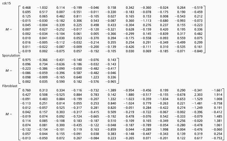
We have determined M, the r × r time translation matrix, for three different data sets of gene expression profiles: yeast cell cycle (CDC15) (20) by using the first 12 equally spaced time points representing the first two cycles, yeast sporulation (21), which has 7 time points, and human fibroblast (22), which has 13 time points (Table 1). The matrix element M_i,j describes the influence of mode j on mode i. Specifically, the coefficient M_i,j multiplied by the expression level of gene j at time t contributes to the expression level of gene i at time (t + Δt). A positive matrix element leads to the ith gene being positively reinforced by the jth gene expression level at a previous time. M is determined exactly and uniquely for the yeast cell-cycle data. The unequal spacing of the time points in the two other data sets precluded an exact solution, and M is an approximation derived by using simulated annealing techniques (27). We have verified that the accuracy of M is very high by showing that the temporal evolution of the modes is reproduced well and that the reconstructed gene expression patterns are virtually indistinguishable from the experimental data. The singular values are spread out, and the amplitudes of the modes decrease as one considers higher-order modes (25). This fact implies that the influence of the dominant modes on the other modes is generally small. Interestingly, for the cdc15 and sporulation data sets, the converse is also true, and the dominant modes are not strongly impacted by the other modes, especially when one takes into account the lower amplitudes of the higher-order modes. This finding suggests that a few-mode approximation ought to be excellent for these two cases.

Table 1.

Time translation matrices

Once the matrix M characterizing the interrelationship between the r modes is determined, it is a simple matter to deduce a matrix that similarly describes the interactions between any other set of r linearly independent profiles. Specifically, one can straightforwardly determine the interrelationships between r clusters of genes. As an example, consider the sporulation data (14), which is characterized by r = 6. The problem of deriving the time translation matrix is underdetermined if the number of clusters exceeds six, and then there is no unique solution. When the number of clusters is less than six, there is no guarantee that there exists even one solution. We therefore consider six clusters (metabolic, early I, early II, middle, midlate, and late), excluding the early-mid cluster, which forms the least coherent group. The average expression patterns of the six clusters (c₁,… ,c₆) are obtained as averages over the genes within the cluster and can be expressed as linear combinations of the six modes as

5

where S is a 6 × 6 matrix. The rows of S are the components of each of the characteristic modes that make up the average expression pattern for the six clusters. The interrelationships between the cluster expression patterns is determined with a time translation matrix of the form

6

so that

7

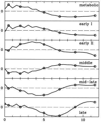
The averages of the experimental measurements (circles) and the predicted expression patterns (lines) of the six clusters are shown in Fig. 1 and are in excellent agreement, confirming the accuracy of the M matrix for the sporulation data in Table 1. The matrix N is shown in Table 2. The significance of the entries in N is similar to that described earlier for M. That is, the matrix element M_i,j describes the influence of cluster j on cluster i. Specifically, the coefficient M_i,j multiplied by the expression level of cluster j at time t contributes to the expression level of cluster i at time (t + Δt). A positive matrix element leads to the ith cluster being positively reinforced by the jth cluster expression level at a previous time.

Figure 1.

A comparison of measured and calculated expression profiles. Average expression profiles for the six clusters of genes in the sporulation data set (14) are represented by circles and the approximated values calculated by using the best-fit time translation matrix are shown as lines.

Table 2.

Time translation matrix for clusters

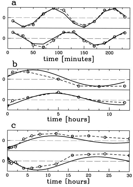
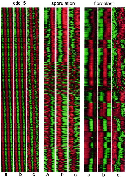
Does one need the full r × r time translation matrix to describe the gene expression patterns? Or is an appropriately chosen truncated time translation matrix adequate to reconstruct the expression patterns with reasonable fidelity? We now consider a linear interaction model (Eq. 2) within which M is a 2 × 2 matrix, and only the two most important modes are used. The values of the four entries in the matrix M are determined by using an optimization scheme that minimizes the cost function similar to that given in Eq. 4. The resulting M matrices are shown in Table 3, and a comparison of the calculated modes (solid lines) with those obtained by SVD (dashed lines) for the three sets of gene expression profiles is shown in Fig. 2. It is interesting to compare these 2 × 2 matrices with the corresponding portion of the full matrices shown in Table 1. The two-mode approximation is excellent for the cdc15 data set (CF = 0.05), moderate for the sporulation data set (CF = 0.18), and not as good for the fibroblast data set (CF = 0.31) as for the others. As noted before, the use of the full r × r time translation matrix leads to an exact reproduction of the data set. Not unexpectedly, the quality of the fit improves as the number of modes considered is increased. Fig. 3 shows the reconstructed expression profiles starting with the initial values, and by using the 2 × 2 time translation matrix (denoted by a), the profiles obtained as a linear combination of the top two modes with appropriate gene-specific coefficients (b) and the experimental data (c) for the three data sets. In all three cases, the main features of the expression patterns are reproduced quite well by the time translation matrix with just two modes. The two-mode reconstruction of the CDC15 profiles is the most accurate of the three.

Table 3.

Effective two-mode time translation matrices

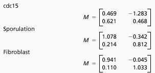Figure 2.

The first two characteristic modes for the (a) cdc15, (b) sporulation, and (c) fibroblast data sets. The circles correspond to the measured data, and the lines show the approximations based on the best-fit 2 × 2 time translation matrices.

Figure 3.

A reconstruction of the expression profiles for the cdc15 (Left), sporulation (Center), and fibroblast (Right) data sets. For each set, a shows the results obtained by using the 2 × 2 time translation matrix to determine the temporal evolution of the expression profiles from their initial values, and b shows expression levels expressed as linear combinations of just the two top modes, whereas c shows the experimental data.

It can be shown that, in general, a 2 × 2 time translation matrix produces only two types of behavior, depending on its eigenvalues. If the eigenvalues are real, the generated modes will independently grow or decay exponentially. When the eigenvalues are complex conjugates of each other, as they are for all three cases we have examined, the two generated modes are oscillatory with growing or decaying amplitudes. Mathematically, the two modes are constrained to have the form:

8

9

Both modes are described by a single time period, τ, and a single growth or decay factor, G. Because there are four parameters in the matrix M, there can be only four independent attributes in the generated modes. Two other parameters, c and Δ, are determined from the initial conditions. In addition to τ and G, we can also determine the phase difference between the two modes, φ, and the relative amplitude of the two modes, A. These attributes can be determined from the coefficients in M by using the equations in Table 4. Table 5 shows the four attributes for each of the three data sets. The self consistency of our analysis is underscored by the fact that the magnitude of the growth factor, G, is close to one for all three cases, which is a biologically pleasing result in that the modes do not grow explosively or decay. For the cell-cycle data, the characteristic period is about 115 min. In the other two cases, the data are not periodic, and hence the best-fit periods are comparable to the duration of the measurement. For the yeast cell-cycle data, φ, the phase difference between the top two modes is 90°, suggesting a simple sine–cosine relationship, as noted by Alter et al. (26). Indeed, this result is self-consistent. When G is equal to 1 and an integer number of periods is considered, orthogonality of the top two modes requires that the phase difference be 90°.

Table 4.

Parameter relationships of the two modes and the effective time translation matrix

Table 5.

Parameter values

	G	A	τ	φ
cdc15	1.008	1.437	115 minutes	90.0°
Sporulation	0.974	1.264	12.8 hours	60.6°
Fibroblast	0.988	0.640	29.2 hours	130.8°

In summary, we have shown that it is possible to describe genetic expression data sets by using a simple linear interaction model with only a small number of interactions. One important implication is that it is impossible to determine the exact interactions among individual genes in these data sets. The problem is underdetermined, because the number of genes is much larger than the number of time points in the experiments. Nonetheless, we have shown that it is possible to accurately describe the interactions among the characteristic modes. Moreover, an interaction model with only two connections reconstructs the key features of the gene expression in the simplest cases with good fidelity. Our results imply that, because there are only a few essential connections among modes and therefore among genes, additional links provide redundancy in the network.

Abbreviation

SVD

singular value decomposition

References

- 1.Pease A C, Solas D, Sullivan E J, Cronin M T, Holmes C P, Fodor S P. Proc Natl Acad Sci USA. 1994;91:5022–5026. doi: 10.1073/pnas.91.11.5022. [DOI] [PMC free article] [PubMed] [Google Scholar]
- 2.Schena M, Shalon D, Davis R W, Brown P O. Science. 1995;270:467–470. doi: 10.1126/science.270.5235.467. [DOI] [PubMed] [Google Scholar]
- 3.Liang S, Fuhrman S, Somogyi R. Pac Symp Biocomput. 1998;3:18–29. [PubMed] [Google Scholar]
- 4.Akutsu T, Miyano S, Kuhara S. Pac Symp Biocomput. 1999;4:17–28. doi: 10.1142/9789814447300_0003. [DOI] [PubMed] [Google Scholar]
- 5.Chen T, He H L, Church G M. Pac Symp Biocomput. 1999;4:29–40. [PubMed] [Google Scholar]
- 6.Szallasi Z. Pac Symp Biocomput. 1999;4:5–16. doi: 10.1142/9789814447300_0002. [DOI] [PubMed] [Google Scholar]
- 7.Weaver D C, Workman C T, Stormo G D. Pac Symp Biocomput. 1999;4:112–123. doi: 10.1142/9789814447300_0011. [DOI] [PubMed] [Google Scholar]
- 8.D'haeseleer P D, Wen X, Fuhrman S, Somogyi R. Pac Symp Biocomput. 1999;4:41–52. doi: 10.1142/9789814447300_0005. [DOI] [PubMed] [Google Scholar]
- 9.van Someren E P, Wessels L F A, Reinders M J T. Proceedings of the Eighth International Conference on Intelligent Systems for Molecular Biology. Menlo Park, CA: AAAI Press; 2000. [PubMed] [Google Scholar]
- 10.Hartwell L H, Hopfield J J, Leibler S, Murray A W. Nature (London) 1999;402:C47–C52. doi: 10.1038/35011540. [DOI] [PubMed] [Google Scholar]
- 11.Jeong H, Tombor B, Albert R, Oltvai Z N, Barabasi A L. Nature (London) 2000;407:651–654. doi: 10.1038/35036627. [DOI] [PubMed] [Google Scholar]
- 12.McAdams H H, Arkin A. Annu Rev Biophys Biomol Struct. 1998;27:199–224. doi: 10.1146/annurev.biophys.27.1.199. [DOI] [PubMed] [Google Scholar]
- 13.McAdams H H, Arkin A. Trends Genet. 1999;15:65–69. doi: 10.1016/s0168-9525(98)01659-x. [DOI] [PubMed] [Google Scholar]
- 14.Bhalla U S, Iyengar R. Science. 1999;283:381–387. doi: 10.1126/science.283.5400.381. [DOI] [PubMed] [Google Scholar]
- 15.Alon U, Surette M G, Barkai N, Leibler S. Nature (London) 1999;397:168–171. doi: 10.1038/16483. [DOI] [PubMed] [Google Scholar]
- 16.Barkai N, Leibler S. Nature (London) 1997;387:913–917. doi: 10.1038/43199. [DOI] [PubMed] [Google Scholar]
- 17.Becskei A, Serrano L. Nature (London) 2000;405:590–593. doi: 10.1038/35014651. [DOI] [PubMed] [Google Scholar]
- 18.Yi T M, Huang Y, Simon M I, Doyle J. Proc Natl Acad Sci USA. 2000;97:4649–4653. doi: 10.1073/pnas.97.9.4649. [DOI] [PMC free article] [PubMed] [Google Scholar]
- 19.Eisen M B, Spellman P T, Brown P O, Botstein D. Proc Natl Acad Sci USA. 1998;95:14863–14868. doi: 10.1073/pnas.95.25.14863. [DOI] [PMC free article] [PubMed] [Google Scholar]
- 20.Spellman P T, Sherlock G, Zhang M Q, Iyer V R, Anders K, Eisen M B, Brown P O, Botstein D, Futcher B. Mol Biol Cell. 1998;9:3273–3297. doi: 10.1091/mbc.9.12.3273. [DOI] [PMC free article] [PubMed] [Google Scholar]
- 21.Chu S, DeRisi J, Eisen M, Mulholland J, Botstein D, Brown P O, Herskowitz I. Science. 1998;282:699–705. doi: 10.1126/science.282.5389.699. [DOI] [PubMed] [Google Scholar]
- 22.Iyer V R, Eisen M B, Ross D T, Schuler G, Moore T, Lee J C F, Trent J M, Staudt L M, Hudson J, Jr, Boguski M S, et al. Science. 1999;283:83–87. doi: 10.1126/science.283.5398.83. [DOI] [PubMed] [Google Scholar]
- 23.Getz G, Levine E, Domany E. Proc Natl Acad Sci USA. 2000;97:12079–12084. doi: 10.1073/pnas.210134797. . (First Published October 17, 2000; 10.1073/pnas.210134797) [DOI] [PMC free article] [PubMed] [Google Scholar]
- 24.Raychaudhuri S, Stuart J M, Altman R. Pac Symp Biocomput. 2000;5:452–463. doi: 10.1142/9789814447331_0043. [DOI] [PMC free article] [PubMed] [Google Scholar]
- 25.Holter N S, Mitra M, Maritan A, Cieplak M, Banavar J R, Fedoroff N V. Proc Natl Acad Sci USA. 2000;97:8409–8414. doi: 10.1073/pnas.150242097. [DOI] [PMC free article] [PubMed] [Google Scholar]
- 26.Alter O, Brown P O, Botstein D. Proc Natl Acad Sci USA. 2000;97:10101–10106. doi: 10.1073/pnas.97.18.10101. . (First Published July 11, 2000; 10.1073/pnas.150242097) [DOI] [PMC free article] [PubMed] [Google Scholar]
- 27.Press W H, Flannery B P, Teukolsky S A, Vetterling W T. Numerical Recipes in C; The Art of Scientific Computing. Cambridge, U.K.: Cambridge Univ. Press; 1992. pp. 444–455. [Google Scholar]