Abstract
An elementary model of animal aggregation is presented. The group-size distributions resulting from this model are truncated power laws. The predictions of the model are found to be consistent with data that describe the group-size distributions of tuna fish, sardinellas, and African buffaloes.
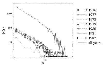
Group formation is a widespread phenomenon throughout the animal kingdom (groups, herds, schools, flocks). Being in group may reduce the chances of being caught by a predator, increase foraging efficiency, reduce energy costs, enhance resistance to toxic environmental conditions, facilitate reproduction, or set the stage for social life (1–4). Groups of animals in general, and fish schools in particular, have been studied from the viewpoint of the behavioral algorithms that govern their formation and dynamics at the individual level (6–9), or from the viewpoint of more macroscopic properties such as group-size distributions (10–13). The probability distribution of group sizes in a given species is an important element for understanding the evolution of grouping in that species; in particular, the existence of a typical group size may suggest that such a size has been selected for because it provides an optimal balance between costs and benefits (14, 15). The notion of optimal group size, however, is problematic: the actual size of a group may be quite different from the size that would be optimal for the group, because it depends on how the group is formed and on what information and power are available to the parties (16, 17). This is especially true for large groups, where the decision for an individual to join a group is likely to rest with that individual, so that group size may eventually be limited only by a maximum group size (10), beyond which an individual is better off alone than in the group. When the maximum size is large, the group-size distribution may exhibit a long tail, a possibility that has been overlooked in virtually all studies (12). Indeed, school size distribution in tropical tuna fish can be well fitted with a truncated power law over 1.5 decades (18): the number N(s) of caught schools of size s follows N(s) ∝ s−b, where b is a scaling exponent, up to a cutoff size sc (Fig. 1). sc sets the scale for the maximum size.
Figure 1.
Log–log plot of N(s) for free-swimming tuna fish schools in which three species, yellowfin tuna (T. albacares), skipjack tuna (K. pelamis), and bigeye tuna (T. obesus) are mixed. Results are given for 7 yr (1976–1982) and for the aggregate distribution of all years. Catch data from the French purse-seine fishery in the tropical Atlantic Ocean (18). s (in tons) is the weight of fish caught in a circular net whose perimeter is about 2 km.
We suggest in this paper that long-tailed (or heavy-tailed) group-size distributions, including power law distributions, may be quite generic. In view of this suggestion, one may ask whether there exist generic proximate mechanisms that produce such distributions. A possible answer to this question lies in a simple model of group formation, arguably the simplest possible model based on elementary cues, inspired by a physical model of particle aggregation (18–20); this model generates group-size distributions that exhibit scaling, that is, power law behavior and slow decay. The model suggests that:
(i) Power law distributions of group sizes result from the basic dynamics of group formation.
(ii) Mean size is not well defined.
(iii) The cutoff size, which plays a role similar to that of a maximum size, depends on detailed characteristics of individual behavior or ecological conditions (food availability, predation, etc.) that do not modify the scale-invariant properties of the size distribution. Such factors influence only the distribution’s cutoff size, its crossover from scale-invariant to rapidly decreasing at large sizes, and possibly its scaling exponent.
(iv) Rapidly decreasing distributions are a limiting case of truncated power laws when the cutoff size becomes small. The continuous process of amalgamation and splitting of diffusing entities leads to a stationary group-size distribution under given ecological and behavioral constraints (10, 12). Previous models accounting for group-size statistics have examined by means of gain–loss equations how the balance between aggregation and splitting under various constraints influences stationary size distributions (10–13). Stability, or instability, results from the competition between aggregation and splitting and their respective characteristic time scales: if splitting is more rapid than aggregation, large groups cannot form. The stability or lack of stability of groups influences the properties of group-size distributions: species with unstable groups tend to be characterized by more rapidly decreasing distributions than species with stable groups.
Why have slowly decaying group-size distributions, including scaling laws, been overlooked in the past, although they are present in many models of group-size statistics (11, 12, 21)? Firstly, power law distributions, D(s) ∝ s−b, where D(s) is the probability that a group be of size s [D(s) is a normalized version of N(s)], do not have a well-defined mean when b ≤ 2, a property that may appear nonbiological. Secondly, in his influential review, Okubo (12) determined that any group-size distribution should be exponentially decreasing by applying a maximum entropy principle to the distribution under the constraint of fixed average size, which implicitly includes the strong assumption that there exists a well-defined mean and therefore overlooks slowly decaying distributions such as power laws with b ≤ 2. It is well known to physicists that such a procedure leads to exponential (Gibbs–Boltzmann) distributions. The detailed balance assumptions, made by Okubo (12), also result in exponential distributions, but such assumptions are not ethologically justified. Thirdly, long-tailed group-size distributions are necessarily truncated at a cutoff size because the population is finite, but truncated power laws must be distinguished from purely rapidly decreasing ones, as they exhibit specific properties (they “violate” the central-limit theorem in practice) (22–24).
The rest of the paper is organized as follows: we first introduce the model and some of its variants, and then present group-size distribution data in fish and African buffaloes that allow the predictions of the model to be tested. The model’s notations are summarized in Table 1.
Table 1.
Summary of notations used in the paper
| Global notations |
| N(s): number of caught schools of size s |
| D(s): probability that a group will be of size s |
| b: exponent of either N(s) or D(s) |
| sc: cutoff size of either N(s) or D(s) |
| d: spatial dimension |
| a, c: fitting parameters for N(s) = a s−be−(s/sc)c |
| General model |
| N: number of sites |
| n: number of simulated individuals |
| Sit: group size at site i at time t |
| Iit: size of group injected into site i at time t |
| Wkit: random hopping variable from site k to site i |
| D(s, t): probability that a group at time t will be of size s |
| Z1(ρ, t): characteristic function of D(s, t) |
| Z1(ρ): characteristic function of D(s) |
| Φ(ρ): characteristic function of Iit |
| 〈Im〉: mth moment of Iit |
| f(x): crossover function of D(s) |
| Splitting models |
| p: fraction of each group splitting at each time step |
| N+: number of sites occupied by a group |
| 〈s′〉: mean group size over all sites |
| 〈s〉: mean group size over occupied sites |
| Psplit(s): probability of splitting for a group of size s |
| σ: maximum allowed group size |
| Model with attracting site |
| η: strength of attraction of the attracting site |
MODEL
General Formulation.
The only assumption underlying the model is the tendency of groups of individuals to aggregate when they meet, an extension of “biosocial attraction” (2–4, 13). This assumption is clearly minimal for a model of group formation. We neglect a lot of parameters—streams, temperature, migratory trends, habitat structure, etc.—to keep the model generic. We assume for modeling purposes that there are N sites, coarse-grained zones of space, on which n individuals move. A single individual is a 1-group; m individuals together form an m-group. One individual may not be the right atomic unit: some species spend most of their time in group, and isolated individuals are rarely observed. A 1-group should then be considered as an atomic object, which may contain a certain number of individuals.
When an m-group and an h-group move to the same site, they aggregate to form an (m + h)-group. At each discrete time step, each group hops to a new site. Simulations show that having groups move asynchronously does not alter the results. We first consider a mean-field approach, where each group hops to a randomly selected site. The mean-field model can apply when there is a large variance in the distance that can be covered within a day.
The equation that describes the dynamics of the group size sit at site i at time t is:
 |
1 |
where Iit represents the injection of new individuals into site i, and Wkit is a random variable representing the motion of a group located at site k at time t toward site i. Wkit can take two values, 0 or 1. We consider that Wkit does not depend on t: Wkit ≡ Wki. Moreover, the Wki are normalized:
 |
2 |
To analyze this model, we now assume that the injection terms Iit are independent equally distributed positive random variables, the exact distribution of which is irrelevant provided it has a finite mean.
RESULTS
Mean-Field Model with No Splitting.
In the simplest mean-field model Wki can be 0 with probability 1 − (1/N) or 1 with probability 1/N. We first assume that groups do not split at all. Let us introduce the characteristic function Z1(ρ, t) of the size distribution D(s, t) at time t (25):
 |
where 〈…〉 denotes the average over all possible realizations of {Wki} (19, 20). In the mean-field case, we have
 |
3 |
where Φ(ρ) ≡ 〈exp[iρIti]〉 is the characteristic function of the injection random variable. To see this, let us write the distribution D(s, t + 1) of s-groups at time t + 1 as a function of D(s, t):
 |
4 |
where sinj is the size of a particular realization of the injection. Eq. 4 arises simply from randomly assembling groups at t + 1. This formula is equivalent to
 |
[simply use the definition of Z1(ρ, t + 1) in terms of D(s, t + 1)], hence the result. Φ(ρ) can be expanded as Φ(ρ) = 1 + i〈I〉ρ − 〈I2〉ρ2/2 + … , where 〈Im〉 is the mth moment of the injection random variable. Taking the limit N → ∞, one obtains the steady-state characteristic function Z1(ρ) = 1 −  〈I〉1/2 |ρ|1/2i−1/2 + … , so that the size distribution satisfies D(s) ∝ s−3/2 for large enough s (s ≫ 〈I〉) (26). It can be shown that the steady-state characteristic function is also an attractor of the dynamical process described above, and that any perturbation is absorbed (27, 28). Simulations confirm that, starting from any initial condition, one converges to the predicted power-law distribution. Because of the constant injection of new individuals, the process is nonstationary and the total number of individuals in the system increases, but this does not prevent a well-defined limit distribution, D(s), from existing. One should also remember that the average size computed with D(s) is infinite. Alternative but related models of coagulation fragmentation, based on a Smoluchowski rate equation including a breakup kernel, are also available with comparable results (21, 29–31).
Mean-Field Model with Splitting.
Simple modifications of the model may affect the critical nature of the process, but the power law behavior is still observed over a finite range. For example, one may observe D(s) ∝ s−3/2e−s/sc [consistent with numerical experiments (29–31)], or more generally D(s) ∝ s−3/2 f(s/sc), where f(x) is a rapidly decreasing crossover function, the particular form of which depends on the detail of the aggregation and breakup processes.
Let us assume that the total number of individuals, n, is constant over time, that a fraction p of each group is separated from the group at each time step, and that the corresponding pn individuals are reinjected into the N sites. The expectation of the injection is then pn/N. D(s, t + 1) is now given by
 |
5 |
because it takes a total size s/(1 − p) hopping onto the same site to get a size s at that site after the removal of a fraction p (it has been assumed for simplicity that removal of particles occurs after injection). We then obtain
 |
6 |
It follows from Eq. 6 that Z1(ρ) =1 − i(s′)ρ + … : the size distribution is short ranged with a finite mean 〈s′〉 = (1 − p)n/N. 〈s′〉 is a mean taken over occupied and empty sites; that is, it includes the statistics of 0-groups. The mean size of groups, 〈s〉, does not include empty sites and is related to 〈s′〉 through 〈s〉 = 〈s′〉N/N+, where N+ is the number of occupied sites. To evaluate N+ in the stationary state, let us write the evolution equation of N+, neglecting encounters of order higher than 2:
 |
7 |
provided N is large enough. Solving for N+, we find that
 |
8 |
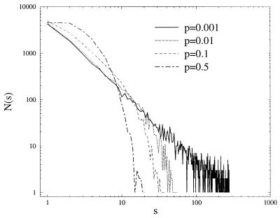
〈s〉 increases when p decreases. The same result can be obtained with another model based on a different formalism (21). In the present case, the total number of individuals being conserved, the mean is finite, but the size distribution D(s) retains some of its power-law characteristics: D(s) ∝ s−3/2 f(s/sc), exhibiting a power law behavior for intermediate sizes 0 ≪ s ≪ 〈s〉. When 〈s〉 is small, the power law is not observed, but only an exponential decay. Simulations have been performed with different values of p. For small values of p, a power law is observed up to a large cutoff size, whereas the distribution is more rapidly decreasing for larger p (Fig. 2: the number N(s) of observed groups of size s is used instead of the normalized value D(s). Here, it appears that f(s/sc) = e−s/sc.
Figure 2.
Log–log plot of N(s). Simulation with n = 100,000 sites, n = 80,000 individuals, P = 0.01, 0.3, 0.5. Simulation run = 106 time steps.
The model explains deviations from power-law behavior through several possible modifications that tend to decrease sc. The cutoff size may result from such factors as some heterogeneity in the speed capacities of the individuals in a group, or, more generally, the ability of a group to maintain its integrity over only a certain amount of time, which itself may depend on ecological conditions and individual behavior. The observed cutoff size in the distribution results from the competition between aggregation and breakup and depends crucially on the time scales associated with aggregation and splitting. For example, the half-life of skipjack tuna schools is likely to be of the order of weeks (32, 33), whereas other fish (12, 34, 35) are occasional schoolers, whose schools are not maintained beyond a minute. In the first case, a power law distribution is observed up to a cutoff size, whereas in the second case the distribution is clearly exponential. Some species exhibit an intermediate strategy between school integrity over long time scales and rapid splitting “pulsating” schools (7) exhibit good cohesion within the day to enhance protection against predators and split in all directions at night (36).
In a similar vein, Gérard and Loisel (37) have shown that the increase of group size with habitat openness in large mammalian herbivores may result simply from the increased opportunity to perceive congeners as habitat openness increases; this increased opportunity in turn increases the probability of group formation, whereas more closed habitats tend to lead to the formation of unstable groups, because individuals may lose their groups more easily. The interplay between the aggregation and splitting time scales leads to a shift toward smaller or larger group sizes: habitat openness plays the role of an ecological parameter constraining the dynamics of aggregation.
The model also makes a prediction that may be important for our understanding of animal groups. Depending on environmental conditions, the stability of groups of a given species may vary; for instance, the lack of food (38), the presence of predators, or bad sea conditions may reduce group stability. If the group-size distribution is a truncated power law, and if the model is relevant to explain the origin of the power law, we expect that such factors affect the cutoff size and not necessarily the power index b.
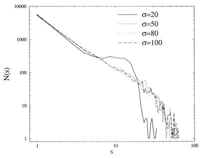
In the previous calculations, it was assumed that all “splitting” individuals were equally redistributed among all sites, but this may not be the case. A group of individuals separating from their group can very well stay together and be reinjected into the system as a whole. The size distribution of splitting groups may also be a parameter on its own, and the probability for a group to split may be related to its size and/or to environmental parameters. But such modifications of the model do not destroy scaling properties. Fig. 3 represents the size distribution obtained from simulations of the mean-field model with P = 0.01 and a splitting probability equal to 1 for any group with a size greater than a maximum allowed size σ (= 20, 50, 80, 100): Psplit(s) = 0 if s σ and Psplit(s) = 1 if s > σ. Although the crossover function f is more complicated than previously, the size distribution exhibits scaling over a certain range that depends on σ, with b = 1.5.
Figure 3.
Same as Fig. 2 with P = 0.01, n = 50,000, n = 80,000 and σ = 20, 50, 80, 100.
Mean-Field Model with Splitting and an Attracting Site.
Introducing a special attracting site, such as a drifting log or an anchored artificial fish-aggregating device (FAD) for fish, or a water hole for mammals, is ethologically relevant and does modify the group-size distribution. A special attraction to site 1 can be included into the model by modifying the probabilities of the transition random variables:
 |
9 |
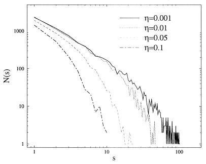
η is a parameter that quantifies the strength of attraction to site 1. Fig. 4 shows how the introduction of this attracting site alters the group-size distribution (at the attracting site). Increasing the attractivity of the site, that is, increasing η, affects the exponent of the distribution and its global shape. Simulations were performed with splitting characterized by P = 0.01. One might argue that introducing a globally attracting site not only introduces an implicit spatial scale, but may also not be realistic. Although this is true, introducing an explicit spatial scale by assuming that only schools within a certain distance of the attracting site are attracted leads to similar results.
Figure 4.
Same as Fig. 2 with P = 0.01 and η = 0, 0.001, 0.01, 0.05, and 0.1.
Spatial Model.
Other exponents can be obtained with more complicated combinations of aggregation and breakup kernels, even in the mean-field case (29–31). But some of the most interesting predictions of the model are related to the effective dimension d of the space in which animals move. Although the ocean is three-dimensional, fish may not use the whole ocean. They may be constrained to swim along the coasts, over the continental shelf, or be limited in depth by physiological constraints, or, alternatively, may move so randomly from any location to any other location that space is irrelevant (mean-field). The same observation is true for many animal species, that, for many reasons, may not fully use their spatial environment.
The exact value of the exponent, in a version of the model on a d-dimensional lattice (groups hop to neighboring sites only) has been obtained by Takayasu et al. (19) for d = 1: b = 4/3. For other dimensions, simulations performed by the same authors indicate that b = 1.465 ± 0.003 for d = 2, b = 1.491 ± 0.007 for d = 3 (19): b increases when d increases. There is a simple explanation for this trend: a small value of b indicates that there are many large groups, which is more likely to happen in low dimension, where groups have a higher probability of meeting and coalescing. Therefore, we expect the exponent b to increase with effective dimension, with a maximum value of b = 3/2, obtained when there is no spatial constraint on movement. The model on a lattice can be generalized to more complicated and realistic models with, for example, tunable fractal dimension: the space in which animals actually move may not have an integer dimension, so that a whole range of exponents may be expected depending on effective space dimension.
Data.
The data presented in this section are catch-per-set data for tuna fish and sardinellas and are direct-count data for African buffaloes. Biases are discussed in the last section of the paper. We are looking for fits of the type N(s) ∝ a s−b f(s/sc), with f(x) = e−xc, where a, b, c and sc are four fitting parameters and f is a crossover function from power law to exponential decay. For simplicity, we restrict our attention to c = 1, 2. We focus here on two points: (i) whether the observed data are consistent with power law distributions, and (ii) whether space dimension influences the size distribution in a way predicted by the model.
We have identified two cases in which the effective dimension may be less than three for fish schools (although the extent of the dimensional reduction that occurs is difficult to quantify accurately): (i) tuna fish in the presence of a drifting log or a FAD, and (ii) some species of sardinellas [clupeid fish (Sardinella maderensis and S. aurita)], which do not make use of the full three-dimensional oceanic space. By contrast, the swimming volume of tuna fish is larger because it is constrained only by large transoceanic ecological boundaries. According to acoustic telemetry experiments (39–41), the common swimming speed for tuna fish is between 0.5 and 2 m⋅s−1, which may correspond to daily covered distances up to 70 km and lead to quite a variance in the locations they can reach, suggesting that the mean-field model may apply. But it is unclear whether free-swimming tuna fish can be adequately described by the mean-field model or by the three-dimensional model. The model predicts that as the effective dimension decreases, one should still observe a power law distribution, with an exponent smaller than the mean-field exponent b = 1.5.
Free-Swimming Tuna.
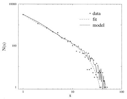
Fig. 5 shows the school size distribution of free-swimming tuna fish (18), aggregated over 7 yr (1976–1982), in which three species, yellowfin tuna (Thunnus albacares), skipjack tuna (Katsuwonus pelamis), and bigeye tuna (T. obesus) are mixed. The dotted line corresponds to a fit of the type s−be−(s/sc)c, with a = 3,497, b = 1.49, c = 2, sc = 29.7 (r > 0.999). The power law is relevant over 1.5 decades. The solid line shows the distribution obtained with the mean-field model with P = 0.1 (r > 0.99). This school size distribution is consistent with both the mean-field model of aggregation (b = 1.5) and the spatial model in three dimensions (b = 1.491).
Figure 5.
School size distribution of free-swimming tuna fish aggregated over 7 yr (same as Fig. 1). The dotted line corresponds to a fit of the type a s−be−(s/sc)c, with a = 3,497, b = 1.49, c = 2, sc = 29.7. The solid line has been obtained with the mean-field model (P = 0.1).
Tuna Fish Schools Caught in the Vicinity of a Fish-Aggregating Device.
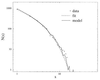
Data originating from fishing performed in the vicinity of a FAD, aggregated over 7 yr (1976–1982) (18) are well fitted by a rapidly decreasing distribution, such as an exponential distribution (Fig. 6). Attraction to the FAD may introduce one or several scales: the probability of a school to be attracted toward the site per unit time introduces a temporal scale, and the distance of attraction of the site, in a spatially explicit model, introduces a spatial scale. However, a power law with a small cutoff size (a s−be−(s/sc)c) is still consistent with the data (dotted line, Fig. 6): a = 1,113.3, b = 0.698, c = 1, sc = 3.72 (r > 0.999) (power law over 0.5 decade). Moreover, such a power law is also consistent with the dimensional reduction that results from the presence of the FAD; it can be argued that the effective dimension is less than 1 because the FAD is a point, so that b should be smaller than 1.3. The solid line in Fig. 6 corresponds to distribution obtained with the mean-field model supplemented with an attracting site, with P = 0.1, n = 80,000, n = 100,000, and η = 0.05.
Figure 6.
School size distribution of tuna fish caught in the vicinity of a FAD aggregated over 7 yr (1976–1982). The dotted line corresponds to a fit of the type a s−be−(s/sc)c, with a = 11,13.3, b = 0.698, c = 1, sc = 3.72. The solid line has been obtained with the mean-field model supplemented with an attracting site (P = 0.1, n = 80,000, n = 100,000, η = 0.05).
Sardinellas.
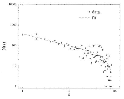
Fig. 7 shows the size distribution of schools of sardinellas (S. maderensis and S. aurita) caught in the upwelling areas of the West African coasts, aggregated over 18 yr (1970–1987) (42). The dotted line represents a fit of the type a s−be−(s/sc)c with a = 503, b = 0.95, c = 2, sc = 59.8 (r > 0.999) (power law over 1.6 decades). This fit is consistent with the dimensional reduction hypothesis. The effective dimension lies between 1 and 2, because sardinellas tend to swim along the coasts above the continental shelf, which reduces the effective dimension by 1. Moreover, the vertical range of this species is also constrained by the depth of the continental shelf, that is, between 1 and 200 m, which further reduces the effective dimension by an unknown factor.
Figure 7.
School size distribution of sardinellas (S. maderensis and S. aurita) caught in the upwelling areas of the West African coasts, aggregated over 18 yr (1970–1987) (42). The dotted line corresponds to a fit of the type a s−b e−(s/sc)c, with a = 503, b = 0.95, c = 2, sc = 59.8.
African Buffaloes.
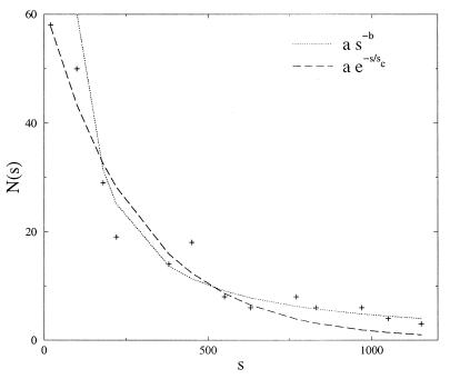
Fig. 8 shows the herd size distribution for the African buffalo (Syncerus caffer) (43). Two fits are represented: one of the form a s−b with a = 9,998 and b = 1.15, and one of the form a e−s/sc, with a = 59 and sc = 297. One unit of s in Fig. 8 corresponds to 10 individuals. The power law seems to match the data in the large size region, whereas the exponential fit is better for small sizes; this result is consistent with the observation that small groups are unstable (disintegration occurs on a faster time scale than aggregation) and large groups are stable (43). Moreover, the b = 1.15 exponent obtained for animals whose movements take place in a two-dimensional space is consistent with the dimensional reduction hypothesis and suggests that the model can apply to terrestrial animals as well. In large vertebrates, such as ungulates, habitat openness, which can be characterized by the fractal dimension of the spatial distribution of open patches, may further reduce the effective dimension because patches of closed habitat (for example, forest patches) prevent individuals from seeing each other and groups from forming (37).
Figure 8.
Herd size distribution of African buffaloes (S. caffer) (43). One unit of s corresponds to 10 individuals). Two fits are represented: one of the form a s−b with a = 9,998 and b = 1.15, and one of the form ae−s/sc with a = 59 and sc = 297.
DISCUSSION
The scaling exponent b clearly decreases when the effective space dimension decreases, which is consistent with the model’s prediction. That the exact values of some of the exponents measured on the empirical data are not in perfect agreement with the values predicted by the model is certainly an issue. It may be explained partly by biases in the data and partly by the fact that small cutoff sizes tend to artificially reduce the estimated value of b.
Let us discuss the biases that exist in the fish data sets. Such biases have never been systematically measured; we assumed that they were consistent across all data sets and did not qualitatively alter the results. There are several ways of estimating school size (acoustic surveys, aerial surveys, light detecting and ranging, catch per set). We use catch per set data because they are easily accessible, relatively inexpensive, and large numbers of observations are available. But a catch made by a purse seiner does not always correspond to an entire school: net saturation leads to an underestimation of school size. Nevertheless, a study based on 18 acoustic surveys of pelagic fish in different tropical areas also indicates that the distribution of school biomass per 1.5 km daytime distance is long tailed and close to a negative exponential function (44). On the other hand, fishermen may not always be interested in small schools, which leads to an underestimation of the number of small schools. Another minor problem is the presence of individuals from different species in a catch, but counting them together, as we have done, may be ethologically relevant because they do school together. Finally, catch-per-set data is expressed in school weight, which is different from the number of individuals. In certain species of fish, such as tuna, there can be large differences between the weights of individuals, and larger fish form heavier schools with fewer individuals, in contrast with small fish, which form large but less heavy schools. The model, however, is rather insensitive to this issue: the mass distribution of the atomic elements is included into the injection term, and the detail of this distribution is irrelevant to the scaling properties, provided the distribution has a well-defined first moment.
The consistency between the ordering of exponents in the empirical data and the ordering predicted by the model is remarkable enough that, despite the factors that bias size estimates, it is a strong evidence that the elementary model of aggregation contains the essential ingredients of animal grouping behavior that influence group-size distribution. The model suggests that long-tailed group-size distributions result from the basic mechanisms of aggregation; there is no need to invoke other mechanisms. Although more data on other animal species are needed, we believe that this model applies to a wide spectrum of cases where group size can be large and aggregation is based on simple cues.
Acknowledgments
E.B. is supported by the Interval Research Fellowship at the Santa Fe Institute. We thank the CRODT Senegal for the sardinella data and J. M. Stretta (Orstom) for the tuna data.
ABBREVIATION
- FAD
artificial fish-aggregating device
References
- 1.Pulliam H R. J Theor Biol. 1973;38:419–438. doi: 10.1016/0022-5193(73)90184-7. [DOI] [PubMed] [Google Scholar]
- 2.Partridge B L. Anim Behav. 1980;28:68–77. [Google Scholar]
- 3.Partridge B L. Sci Am. 1982;245:114–123. doi: 10.1038/scientificamerican0682-114. [DOI] [PubMed] [Google Scholar]
- 4.Shaw E. In: Development and Evolution of Behavior. Aronson L, editor. San Francisco: Freeman; 1970. [Google Scholar]
- 5.Aoki I. Bull Jpn Soc Sci Fish. 1982;48:1081–1088. [Google Scholar]
- 6.Aoki I. Bull Jpn Soc Sci Fish. 1986;52:1115–1119. [Google Scholar]
- 7.van Winkle W, Rose K A, Chambers R C. Trans Am Fish Soc. 1993;122:397–403. [Google Scholar]
- 8.Niwa H-S. J Theor Biol. 1994;171:123–136. [Google Scholar]
- 9.Seno H. Ecol Modell. 1990;51:217–226. [Google Scholar]
- 10.Duffy D C, Wissel C. Ecol Modell. 1988;40:201–211. [Google Scholar]
- 11.Anderson J J. U S Fish Bull. 1981;79:315–323. [Google Scholar]
- 12.Okubo A. Adv Biophys. 1986;22:1–94. doi: 10.1016/0065-227x(86)90003-1. [DOI] [PubMed] [Google Scholar]
- 13.Swartzman G. Ecol Modell. 1991;56:63–80. [Google Scholar]
- 14.Pitcher T J, Parrish J K. In: The Behavior of Teleost Fishes. 2nd Ed. Pitcher T J, editor. London: Chapman & Hall; 1993. pp. 363–439. [Google Scholar]
- 15.Giraldeau L A. In: The Ecology of Social Behavior. Slobodchikoff C N, editor. New York: Academic; 1988. pp. 33–53. [Google Scholar]
- 16.Sibly R M. Anim Behav. 1983;31:947–948. [Google Scholar]
- 17.Clark C, Mangel M. Am Nat. 1984;123:626–641. [Google Scholar]
- 18.Bonabeau E, Dagorn L. Phys Rev E. 1995;51:5220–5223. doi: 10.1103/physreve.51.r5220. [DOI] [PubMed] [Google Scholar]
- 19.Takayasu H, Nishikawa I, Tasaki H. Phys Rev A. 1988;37:3110–3117. doi: 10.1103/physreva.37.3110. [DOI] [PubMed] [Google Scholar]
- 20.Takayasu H. Phys Rev Lett. 1989;63:2563–2565. doi: 10.1103/PhysRevLett.63.2563. [DOI] [PubMed] [Google Scholar]
- 21.Gueron S, Levin S A. Math Biosci. 1995;128:243–264. doi: 10.1016/0025-5564(94)00074-a. [DOI] [PubMed] [Google Scholar]
- 22.Mantegna R N, Stanley H E. Phys Rev Lett. 1994;73:2946–2949. doi: 10.1103/PhysRevLett.73.2946. [DOI] [PubMed] [Google Scholar]
- 23.Mantegna R N, Stanley H E. Nature (London) 1995;376:46–49. [Google Scholar]
- 24.Koponen I. Phys Rev E. 1995;52:1197–1199. doi: 10.1103/physreve.52.1197. [DOI] [PubMed] [Google Scholar]
- 25.Feller W. An Introduction to Probability Theory and Its Applications. 2nd Ed. I. New York: Wiley; 1957. [Google Scholar]
- 26.Montroll E, Bendler J T. J Stat Phys. 1984;34:129–162. [Google Scholar]
- 27.Takayasu H, Provata A, Takayasu M. Phys Rev A. 1990;42:7087–7090. doi: 10.1103/physreva.42.7087. [DOI] [PubMed] [Google Scholar]
- 28.Takayasu H, Takayasu M, Provata A, Huber G. J Stat Phys. 1991;65:725–745. [Google Scholar]
- 29.Family F, Meakin P, Deutch J M. Phys Rev Lett. 1986;57:727–730. doi: 10.1103/PhysRevLett.57.727. [DOI] [PubMed] [Google Scholar]
- 30.Meakin P, Ernst M H. Phys Rev Lett. 1988;60:2503–2506. doi: 10.1103/PhysRevLett.60.2503. [DOI] [PubMed] [Google Scholar]
- 31.Edwards B F, Cai M, Han H. Phys Rev A. 1990;41:5755–5757. doi: 10.1103/physreva.41.5755. [DOI] [PubMed] [Google Scholar]
- 32.Lester R J G, Barnes A, Habib B. Fish Bull. 1985;83:343–356. [Google Scholar]
- 33.Bayliff W H. Fish Bull. 1988;86:631–643. [Google Scholar]
- 34.Seghers B H. Environ Biol Fishes. 1981;6:21. [Google Scholar]
- 35.Breder C M. Zoologica (NY) 1967;52:25. [Google Scholar]
- 36.Fréon P, Gerlotto F, Soria M. ICES J Mar Sci. 1996;53:363–372. [Google Scholar]
- 37.Gérard J-F, Loisel P. J Theor Biol. 1995;176:511–522. [Google Scholar]
- 38.Morgan M J. J Fish Biol. 1988;32:963–971. [Google Scholar]
- 39.Cayré P, Chabanne J. Océanogr Trop. 1986;21:167–183. [Google Scholar]
- 40.Holland K N, Brill R W, Chang R K C. Fish Bull. 1990;88:493–507. [Google Scholar]
- 41.Cayré P. Aquat Liv Res. 1991;4:1–12. [Google Scholar]
- 42.Fréon P, Levenez J-J, Sow I. In: L’Evaluation des Ressources Exploitables par la Pêche Artisanale Sénégalaise. Barry G, Diouf T, Fonteneau A, editors. Paris: Orstom Editions; 1994. [Google Scholar]
- 43.Sinclair A R E. The African Buffalo. Chicago: Univ. Chicago Press; 1977. [Google Scholar]
- 44.Fréon P, Soria M, Mullon C, Gerlotto F. Aquat Liv Res. 1993;6:221–234. [Google Scholar]


