

Abstract
As biological studies shift from molecular description to system analysis we need to identify the design principles of large intracellular networks. In particular, without knowing the molecular details, we want to determine how cells reliably perform essential intracellular tasks. Recent analyses of signaling pathways and regulatory transcription networks have revealed a common network architecture, termed scale-free topology. Although the structural properties of such networks have been thoroughly studied, their dynamical properties remain largely unexplored. We present a prototype for the study of dynamical systems to predict the functional robustness of intracellular networks against variations of their internal parameters. We demonstrate that the dynamical robustness of these complex networks is a direct consequence of their scale-free topology. By contrast, networks with homogeneous random topologies require fine-tuning of their internal parameters to sustain stable dynamical activity. Considering the ubiquity of scale-free networks in nature, we hypothesize that this topology is not only the result of aggregation processes such as preferential attachment; it may also be the result of evolutionary selective processes.
Complex protein and genetic networks are large systems of interacting molecular elements that control the propagation and regulation of various biological signals (1–3). They constitute essential classes of biological computations reflecting vital cellular processes such as the regulation of the cell cycle and gene expression. Because some intracellular processes are crucial for the survival of the cell they need to be achieved with reliability. For example, the variation of the concentration of network components in a metabolic network may affect numerous processes. The intricate architecture of such networks raises the question of the stability of their functioning. How can such complex dynamical systems achieve important cellular tasks and remain stable against the variations of their internal parameters?
Three decades ago, Savageau (4, 5) hypothesized that robustness was an essential property of some genetic networks whose functioning would be preserved even if some of their components were produced in various quantities. More recently, several compelling theoretical (6, 7) and experimental (8, 9) studies demonstrated that key processes of specific intracellular networks exhibited a robust behavior to variations of biochemical parameters. Robustness has emerged as a fundamental concept for the characterization of the dynamical stability of biological systems.
Are there universal design principles that would determine whether a given class of networks achieves important intracellular processing with reliability (10)? It would then be possible to predict dynamical properties underlying cell functions without a full knowledge of the molecular details. In particular, it would be important to characterize dynamical robustness as the ability for the network to perform a sequence of biological tasks in the presence of perturbations (3). Driven by such considerations, we analyzed when dynamical robustness may be a direct consequence of the network's architecture.
As a test-bed for the study of the dynamical properties of complex biological networks we chose to model molecular activities by a simple two-state model closely related to the one proposed by Kauffman (11, 12). This model was originally created for the study of the dynamics of genetic networks, but was later applied to evolution and social models and became a prototype for the study of dynamical systems. In this model, the network's architecture follows a random topology in which every element interacts, on average, with K other elements. Each network element has two functional states, active and inactive. The state of a given element is determined by its interactions with other elements of the network (see Appendix). A generic biochemical parameter for the whole system is the probability ρ that an arbitrary element of the network becomes active after interacting with other elements (13). This probability can be inferred in principle from the reaction rates and the relative concentration of each element. The nature of the dynamical process performed by a given network is determined by its topological parameter K and its biochemical parameter ρ. Under the simple assumption of a random network topology, a very rich and unexpected dynamical behavior of the network was found (11, 12, 14). During the time evolution of the system, the network elements pass through different states until they reach a cyclic behavior. Different cycles are possible. Each cycle represents a variety of intracellular tasks. Two regimes of network activity exist: chaotic and robust. In the chaotic regime a perturbation in the state of a single element can make the system jump from one cycle to another. In the robust regime all such perturbations die out over time. The transition from one regime to the other is controlled by the parameters K and ρ and is determined by the equation
 |
[1] |
Fig. 1a defines the two regimes of network activity with drastically different dynamical properties. In the chaotic regime, which entirely dominates the parameter space (K-ρ), small variations of the initial concentration of only one component would ruin the network function. Conversely, the robust regime would give rise to a reliable dynamics for which the network activity would be insensitive to perturbations in the initial state of the network elements. With a random network topology this regime is attained only for a narrow range of the parameters K and ρ.
Fig. 1.

Dynamical robustness of a Boolean network with random topology. (a) The network dynamics exhibit both chaotic and robust behaviors, depending on the value of the parameters K and ρ. The parameter space K-ρ is then divided into two distinct regimes: chaotic (white) and robust (gray). The curve separating these two regimes is given by the solutions of Eq. 1. For a random network topology (Inset), the parameter space K-ρ is totally dominated by the chaotic regime. Therefore, it is necessary to fine-tune the parameters K and ρ to achieve robust dynamics. (Inset) A typical realization of the random network topology, generated by using a Poisson distribution with K = 2. All elements in the network (•) have approximately the same number of input elements (○). (b) The dynamical robustness R of the network is defined as the fraction of the interval (0,1) for which the parameter ρ gives rise to networks with a robust behavior. This quantity is a function of the mean connectivity K and decreases rapidly a K increases. For a moderate connectivity K = 20, the dynamical robustness is ≈R = 5%.
Unfortunately, this model is inadequate to account for the functioning of biological networks that have heterogeneous architecture. Such topological heterogeneity is present in the human genome. For example, the expression of the β-globin gene is controlled by >20 regulatory proteins. The fibroblast or the platelet-derived growth factor activation induces the activation of >60 other genes (15). Also, the zinc-finger protein Sp1 controls the expression of >300 genes (16). Under an assumption of a random homogeneous architecture with a mean connectivity K = 20, robust behavior would be virtually attained only for ≈5% of the possible values of ρ. Fig. 1b shows the fraction of the interval (0,1) for which the parameter ρ gives rise to networks with a robust behavior. It is apparent that for a random topology only the fine-tuning of the parameters K and ρ in a narrow interval would allow networks to operate with a robust behavior. An alternative approach is to substitute the random network topology for a more realistic one (17).
In recent years, the analyses of the topology of large intracellular networks have revealed a common architecture (18–20). In these natural networks not all elements are equivalent. A small, but significant, fraction of the elements are highly connected, whereas the majority of the elements are poorly connected. This architecture is called scale-free topology and was found to be ubiquitous in networks as diverse as social (21), ecological (22), and genetic, protein networks (18, 23), and the World Wide Web (24, 25). Although the effect of deleterious perturbations on the topology of these networks has been thoroughly studied (23, 26), their dynamical properties need to be explored.
In view of the ubiquity of scale-free networks in nature, we chose to implement the scale-free topology into the two-state model. This topology is defined such that the probability P(k) that an arbitrary element of the networks interacts with exactly k other elements follows the power law P(k) = [Z(γ)kγ]–1. The parameter γ is called the scale-free exponent, and Z(γ) is the normalization factor. When γ increases both the fraction of highly connected elements and the mean connectivity of the network decrease. In the limit γ → ∞ the network becomes a homogeneous random network with K = 1.
Our approach aims to characterize how the network architecture shapes its dynamical properties and how one particular topology favors a class of networks with robust dynamical behavior (10). Although the average connectivity K is a relevant parameter to characterize the homogeneous topology of random networks, it becomes irrelevant to describe the highly heterogeneous scale-free topology. Thus, the only relevant parameter that characterizes the architecture of scale-free networks is the scale-free exponent γ.
For networks with scale-free topology, the transition from chaotic to robust dynamics is determined by the equation (see Appendix)
 |
[2] |
The values of γ and ρ that satisfy this transcendental equation are plotted on Fig. 2a. The results of our model reported in the diagram reveal a large class of robust networks. This class is defined for networks with topological parameters γ > 2. These networks can operate with a robust dynamical behavior for which the mean biochemical parameter ρ spans over a large range of values. In particular, networks with a parameter γ > 2.5 would display a robust dynamics for any value of ρ. The transition from the chaotic to the robust regimes occurs for values of γ in the interval [2,2.5] and different values of ρ. Fig. 2a reveals another class of networks with a topological parameter γ < 2 that exhibit chaotic behavior. This dynamical behavior is characterized by an extreme sensitivity to small variations of the initial states of the network elements. Our model shows that the emergence of a large class of robust networks is a direct consequence of the network architecture.
Fig. 2.

Dynamical robustness of a Boolean network with scale-free topology. (a) The mean connectivity K is not a relevant parameter to characterize the network topology for a scale-free network. The dynamics is then characterized in terms of the parameters γ and ρ, where γ is the scale-free exponent. The parameter space γ-ρ is divided in two distinct regimes: chaotic (white) and robust (gray). The transition between these two regimes, given by Eq. 2, is represented here by the solid curve. The chaotic regime does not longer dominate the parameter space. (Inset) A typical realization of the scale-free topology, generated by using a power-law distribution with λ = 2.5. The majority of the elements only have a few connections. But there are two elements connected to almost all other elements in the system. (b) Dynamical robustness R as a function of the scale-free exponent γ. The transition from the chaotic to the robust regime occurs in the interval [2, 2.5]. For γ > 2.5 the dynamics is robust for any value of ρ. The scale-free topology does not require fine-tuning of the parameters γ and ρ to achieve stability. (c) Histogram of 46 scale-free exponents reported for a wide collection of scale-free networks. This collection includes not only biological networks, but also social, ecological, and informatics networks (23, 30–33). It is interesting to note that the majority of the exponents belong to the interval (2, 2.5) where the transition from a robust to a chaotic behavior occurs.
It is interesting to note that experimental values of γ, extracted from real intracellular networks, range in the interval [2, 2.5]. To illustrate this general remark, we indiscriminately report on a histogram 46 published values of scale-free exponents (Fig. 2c). These values were obtained not only from real biological systems but also from many other scale-free networks (20, 23, 25). Remarkably, the majority of these exponents fall in the predicted interval where the transition from chaotic to robust behavior occurs.
This observation leads us to explore the dynamical response of the network to perturbations in the three different regimes: chaotic, critical, and robust. In a scale-free network not all elements are equivalent. We do not expect that perturbing highly connected elements have the same effect on the network dynamics than perturbing poorly connected elements. To test this idea we analyzed numerically how a perturbation produced on only one element affects the dynamics of the network. We computed the overlap (see Appendix) between two trajectories. One trajectory is computed with one element σi with ki connections being perturbed at every time step of the temporal evolution of the network. The second trajectory is computed from the same initial condition but with no perturbation. Such overlap is a measure of the dynamical stability of the system under sustained perturbations. Fig. 3 shows that the stability of the network decreases with the connectivity ki of the perturbed element σi. Remarkably, we found that networks operating in the robust regime are sensitive to perturbations applied to the highly connected elements. In contrast, perturbations produced on arbitrary elements, which in general are poorly connected, will have little effect on the network functioning. The heterogeneity of scale-free networks operating in the robust regime allows different dynamical responses to perturbations depending on the particular element being perturbed. This behavior cannot be observed in homogeneous random networks in which all of the elements are equivalent.
Fig. 3.

Dynamical stability of scale-free networks. The overlap between a perturbed trajectory and an unperturbed trajectory is computed. Both trajectories start out from the same initial configuration. In the perturbed trajectory one element σi with ki connections randomly takes the values 0 and 1 with the same probability, regardless of the configuration of its input elements. All of the other elements for this trajectory are updated according to Eq. A.1. For the unperturbed trajectory all of the elements follow the dynamics given by Eq. A.1. The graph shows the overlap x between the perturbed and the unperturbed trajectories as a function of the connectivity ki of the perturbed element σi. The different curves correspond to the three different regimes: chaotic (γ = 1.1), critical (γ = 2.5), and robust (γ = 4). In these three cases ρ = 0.5. The simulation was carried out for networks with N = 20 elements. Each point represents the average over 20,000 network realizations.
For a homogeneous network topology, stable behavior was achieved only for very restricted values of the parameters ρ and K. Conversely, the scale-free topology does not require a fine-tuning of the system parameters to attain robustness. This topology allows the existence of robust dynamics in heterogeneous networks. Furthermore, the dynamics of scale-free networks can change if the highly connected elements are perturbed. Thus, scale-free networks operating in the robust regime exhibit both, robustness and sensitivity to perturbations. The above results suggest that the dynamical robustness of a wide variety of biological processes may be a direct consequence of the network architecture. The ubiquity of scale-free networks in nature with a topological parameter 2 < γ < 3 could be the result of evolutionary processes (27). Such a large class of networks, whose key dynamical processes are robust, may have an essential evolutionary advantage in possessing a larger parameter space to adapt to new environmental conditions (27, 28). In our opinion, it would be surprising if nature did not exploit this convenient dynamical property of the scale-free topology.
This work describes the dynamics of networks where complex molecular activities are idealized with a two-state model (29). There exists a fair number of intracellular regulatory systems with components obeying the rules of a two-state model. For example, in signal transduction networks, the signal is processed through phosphorylation cascades where signaling molecules can be active or inactive upon phosphorylation. It is also common to describe regulatory transcription networks in this simple language: A transcription factor regulates positively or negatively the transcription of a given gene. Moreover, available data on the activity of molecular components from large intracellular networks are produced by high-throughput experiments such as two-hybrid assays and C-DNA microarrays. Because of technical constraints, the readout of these experiments is fashioned accordingly to a two-state format that facilitates the applicability of our approach.
The identification of a relationship between topology and dynamical properties of large biological networks primarily motivated our work. But it seems appropriate to think that in view of the significance of scale-free networks in other fields such as sociology and economics our results could be of some interest beyond the scope of biology.
Acknowledgments
We thank Leo P. Kadanoff, Leo Silbert, Tao Pan, Tamara Griggs, and Calin Guet for useful comments. This work was supported by the Materials Research Science and Engineering Center program of the National Science Foundation under Award 9808595 and National Science Foundation Grant DMR 0094569. M.A. also acknowledges the Santa Fe Institute of Complex Systems for partial support through the David and Lucile Packard Foundation Program in the Study of Robustness.
Appendix
A Boolean network is represented by a set of N elements, {σ1, σ2,..., σN}. Each element has two possible states: active (1) or inactive (0). The value of each σi is controlled by ki other elements of the network (see Fig. 4), where ki is a random variable chosen from a probability distribution P(k). This probability distribution determines the topology of the network. We define K as the mean value of P(k). Let {σi1, σi2,..., σiki} be the set of controlling elements of σi. We then assign to each σi a Boolean function fi(σi1, σi2,..., σiki). For each configuration of the controlling elements, fi(σi1, σi2,..., σiki) = 1 with probability ρ and fi(σi1, σi2,..., σiki) = 0 with probability 1 – ρ. Once the controlling elements and the Boolean functions have been assigned to every element in the network, the dynamics of the system are given by
 |
[A.1] |
We will denote as Σ(t) the configuration of the entire system at time t: Σ(t) = {σ1(t), σ2(t),..., σN(t)}.
Fig. 4.

Schematic representation of the Kauffman model. Every element σi receives inputs from ki other elements of the network. The ki inputs of σi are chosen randomly from anywhere in the system. In the case shown, ki = 4.
The dynamical robustness of the network is analyzed by considering the
trajectories Σ(0) → Σ(1) → · · ·
→ Σ(t) and
 →
→
 → · ·
· →
→ · ·
· →  produced by
two slightly different initial configurations, Σ(0) and
produced by
two slightly different initial configurations, Σ(0) and
 , respectively. These
trajectories can always be different under the temporal evolution of the
system, or they can eventually converge to the same trajectory. An important
quantity that reveals the robustness of the dynamics against perturbations in
the initial configuration is the overlap between Σ(t) =
{σ1(t), σ2(t),...,
σN(t)} and
, respectively. These
trajectories can always be different under the temporal evolution of the
system, or they can eventually converge to the same trajectory. An important
quantity that reveals the robustness of the dynamics against perturbations in
the initial configuration is the overlap between Σ(t) =
{σ1(t), σ2(t),...,
σN(t)} and
 ,
defined as
,
defined as
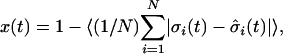 |
where 〈·〉 represents the average over all possible initial configurations and network realizations. If limt→∞ x(t) = 1, all perturbations in a given initial configuration die out over time (robust behavior). In contrast, if limt→∞ x(t) ≠ 1 even small perturbations in the initial configuration propagate across the entire system and never disappear (chaotic behavior).
It has been shown in ref. 17 that for a large system (N → ∞), the temporal evolution of the overlap is given by
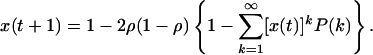 |
[A.2] |
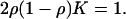
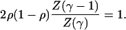
In the limit t → ∞ the above equation becomes a fixed-point equation for the stationary value of the overlap x = limt→∞x(t). It follows from Eq. A.2 that if 2ρ(1 – ρ)K ≤ 1, the only stable fixed point is x = 1 [K is mean value of P(k)]. In this case the system is in the robust regime. On the other hand, if 2ρ(1 – ρ)K > 1 there is a stable fixed point x ≠ 1 and the dynamics of the network are chaotic. The critical value Kc of the mean connectivity at which the transition from robust to chaotic dynamics occurs is given as a function of ρ by the equation
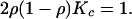 |
[A.3] |
The values of Kc and ρ that satisfy this
equation are plotted on Fig. 1.
It is interesting to note that the transition from robust to chaotic dynamics
is governed by K, the mean value of P(k). However,
this parameter is meaningful only when the distribution P(k)
has a well-defined variance. In this case the fluctuations in the number of
connections of the individual elements around the mean connectivity K
are bounded. This is actually the case when P(k) is a
Poissonian or a Gaussian distribution. For these distributions the mean
connectivity K is the relevant parameter that characterizes the
network topology. Originally Kauffman
(11,
12) proposed this model under
the assumption that K is a relevant parameter. However, the variance
of the scale-free distribution P(k) =
[Z(γ)kγ]–1
is infinite for γ ≤ 3. This means that the actual number of
connections of the individual elements can vary from 1 up to N.
Consequently, the mean value of the connectivity is no longer a meaningful
parameter to characterize the network topology. For a highly heterogeneous
network with scale-free topology, the only relevant parameter that
characterizes the network topology is the scale-free exponent γ itself.
For these kinds of networks it is better to represent the mean connectivity
K as a function of the scale-free exponent γ, which gives
K = Z(γ – 1)/Z(γ). In the above
expression
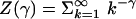 is the Riemann Zeta function. With this representation, the transition from
robust to chaotic behavior is then given by
is the Riemann Zeta function. With this representation, the transition from
robust to chaotic behavior is then given by
 |
[A.4] |
The values of γ and ρ for which this transcendental equation is satisfied are plotted on Fig. 2.
The network that we have considered is a directed graph. The value of each element σi is controlled by a set of ki elements. But σi can in turn control the values of a number of other elements. Therefore, each element has a set of input connections and a set of output connections. The number of inputs and outputs of each element are not necessarily distributed with the same probability distribution P(k). However, the total number of inputs in the network equals the total number of outputs, so that on average, every element has the same number of inputs than outputs. Because the phase transition is governed only by the first moment of P(k), it follows that Eq. A.4 is valid if either the distribution of input connections or that of the output connections (or both) is scale free.
This paper was submitted directly (Track II) to the PNAS office.
References
- 1.Hartwell, L. H., Hopfield, J. J., Leibler, S. & Murray, A. W. (1999) Nature 402, C47–C52. [DOI] [PubMed] [Google Scholar]
- 2.Kitano, H. (2002) Science 295, 1662–1664. [DOI] [PubMed] [Google Scholar]
- 3.Ideker, T., Thorsson, V., Ranish, J. A., Christmas, R., Buhler, J., Eng, J. K., Bumgarner, R., Goodlett, D. R., Aebersold, R. & Hood, L. (2001) Science 292, 929–934. [DOI] [PubMed] [Google Scholar]
- 4.Savageau, M. A. (1971) Nature 229, 542–544. [DOI] [PubMed] [Google Scholar]
- 5.Savageau, M. A. (1975) Nature 258, 208–214. [DOI] [PubMed] [Google Scholar]
- 6.Yi, T. M., Huang, Y., Simon, M. I. & Doyle, J. (2000) Proc. Natl. Acad. Sci. USA 97, 4649–4653. [DOI] [PMC free article] [PubMed] [Google Scholar]
- 7.Barkai, N. & Leibler, S. (1997) Nature 387, 913–917. [DOI] [PubMed] [Google Scholar]
- 8.Alon, U., Surette, M. G., Barkai, N. & Leibler, S. (1999) Nature 397, 168–171. [DOI] [PubMed] [Google Scholar]
- 9.Eldar, A., Dorfman, R., Weiss, D., Ashe, H., Shilo, B. Z. & Barkai, N. (2002) Nature 419, 304–308. [DOI] [PubMed] [Google Scholar]
- 10.Fox, J. J. & Hill, C. C. (2001) Chaos 11, 809–815. [DOI] [PubMed] [Google Scholar]
- 11.Kauffman, S. A. (1969) Nature 224, 177–178. [DOI] [PubMed] [Google Scholar]
- 12.Kauffman, S. A. (1969) J. Theor. Biol. 22, 437–467. [DOI] [PubMed] [Google Scholar]
- 13.Luque, B. & Sole, R. V. (1997) Phys. Rev. E Stat. Phys. Plasmas Fluids Relat. Interdiscip. Top. 55, 257–260. [Google Scholar]
- 14.Derrida, B. & Stauffer, D. (1986) Europhys. Lett. 2, 739–745. [Google Scholar]
- 15.Huang, S. & Ingber, D. E. (2000) Exp. Cell Res. 261, 91–103. [DOI] [PubMed] [Google Scholar]
- 16.Zuber, J., Tchernitsa, O. I., Hinzmann, B., Schmitz, A. C., Grips, M., Hellriegel, M., Sers, C., Rosenthal, A. & Schafer, R. (2000) Nat. Genet. 24, 144–152. [DOI] [PubMed] [Google Scholar]
- 17.Oosawa, C. & Savageau, M. A. (2002) Phys. D 170, 143–161. [Google Scholar]
- 18.Jeong, H., Tombor, B., Albert, R., Oltval, Z. N. & Barabasi, A. L. (2000) Nature 407, 651–654. [DOI] [PubMed] [Google Scholar]
- 19.Jeong, H., Mason, S. P., Barabasi, A. L. & Oltvai, Z. N. (2001) Nature 411, 41–42. [DOI] [PubMed] [Google Scholar]
- 20.Ravasz, E., Somera, A. L., Mongru, D. A., Oltvai, Z. N. & Barabasi, A. L. (2002) Science 297, 1551–1555. [DOI] [PubMed] [Google Scholar]
- 21.Newman, M. E. J. (2001) Proc. Natl. Acad. Sci. USA 98, 404–409. [DOI] [PMC free article] [PubMed] [Google Scholar]
- 22.Sole, R. V. & Montoya, J. M. (2001) Proc. R. Soc. London Ser. B 268, 2039–2045. [DOI] [PMC free article] [PubMed] [Google Scholar]
- 23.Maslov, S. & Sneppen, K. (2002) Science 296, 910–913. [DOI] [PubMed] [Google Scholar]
- 24.Albert, R., Jeong, H. & Barabasi, A. L. (1999) Nature 401, 130–131. [Google Scholar]
- 25.Strogatz, S. H. (2001) Nature 410, 268–276. [DOI] [PubMed] [Google Scholar]
- 26.Albert, R., Jeong, H. & Barabasi, A. L. (2000) Nature 406, 378–382. [DOI] [PubMed] [Google Scholar]
- 27.Kauffman, S. A. & Smith, R. G. (1986) Phys. D 22, 68–82. [Google Scholar]
- 28.Kauffman, S. A. (1990) Phys. D 42, 135–152. [Google Scholar]
- 29.Kauffman, S. A. (1984) Phys. D 10, 145–156. [Google Scholar]
- 30.Albert, R. & Barabasi, A. L. (2002) Rev. Mod. Phys. 74, 47–97. [Google Scholar]
- 31.Rzhetsky, A. & Gomez, S. M. (2001) Bioinformatics 17, 988–996. [DOI] [PubMed] [Google Scholar]
- 32.Cancho, R. F. I. & Sole, R. V. (2001) Proc. R. Soc. London Ser. B 268, 2261–2265. [Google Scholar]
- 33.Pastor-Satorras, R., Vazquez, A. & Vespignani, A. (2001) Phys. Rev. Lett. 87, 258701. [DOI] [PubMed] [Google Scholar]