Approximate Genealogies Under Genetic Hitchhiking

Abstract

The rapid fixation of an advantageous allele leads to a reduction in linked neutral variation around the target of selection. The genealogy at a neutral locus in such a selective sweep can be simulated by first generating a random path of the advantageous allele's frequency and then a structured coalescent in this background. Usually the frequency path is approximated by a logistic growth curve. We discuss an alternative method that approximates the genealogy by a random binary splitting tree, a so-called Yule tree that does not require first constructing a frequency path. Compared to the coalescent in a logistic background, this method gives a slightly better approximation for identity by descent during the selective phase and a much better approximation for the number of lineages that stem from the founder of the selective sweep. In applications such as the approximation of the distribution of Tajima's D, the two approximation methods perform equally well. For relevant parameter ranges, the Yule approximation is faster.

THE model of genetic hitchhiking, introduced in Maynard Smith and Haigh (1974), has become an increasingly important tool for detecting loci under strong positive directional selection in a genome (Nurminsky 2005). During the fixation of a beneficial allele, neutral variation around the target of selection is partially eliminated. This leads to the reduction of sequence diversity at neutral loci linked to a site under strong positive selection, a phenomenon known as a selective sweep. The reduction of diversity can be used to infer regions in the genome affected by selection in the recent past (Sabeti et al. 2002; Glinka et al. 2003; Beisswanger et al. 2006).

A reduction in sequence diversity caused by a selective sweep can be observed only if selection is strong, linkage between a neutral marker and the selective site correlates the histories of the selected and the neutral locus, and the fixation of the beneficial allele is recent. On the one hand the rare coincidence of these three factors restricts the number of selective sweeps in sequence data. On the other hand the reduction in diversity is easy to observe, which makes selective sweeps a powerful tool for detecting selected regions even if functional information is absent.

A detailed analysis of the diversity patterns caused by genetic hitchhiking leads to a deeper understanding of the effect of underlying evolutionary forces. This can be used to predict how well tests of neutrality perform under strong directional selection and to differentiate between sequence data obtained under strong directional selection and under other demographic scenarios. After the first description of the hitchhiking effect by Maynard Smith and Haigh (1974), several authors have attempted to approximate the diversity pattern that is formed by a selective sweep (Kaplan et al. 1989; Stephan et al. 1992; Barton 1998; Durrett and Schweinsberg 2004; Etheridge et al. 2006).

Initiated by the “revisiting” of the hitchhiking effect by Kaplan et al. (1989), coalescent theory has helped to understand diversity patterns formed by selective sweeps: the ancestry of a sample at a neutral locus that is linked to the selected one is modeled as a structured coalescent; its background is the frequency curve of the selectively advantageous allele that increases from 0 to 1 during the sweep. To account for all random effects in a finite population, one would ideally model the evolution of this frequency curve by a Wright–Fisher process with selection and use the structured coalescent with recombination in this background. However, simulation of this stochastic model is prohibitively slow, especially for large populations.

For this reason, several approximations of the Wright–Fisher model have been proposed. Most influential has been the idea that for strong selection the increase in frequency of the beneficial allele is almost deterministic. Kaplan et al. (1989) suggested that the evolution of the frequency of the beneficial allele in a selective sweep can be described by a logistic curve and that this curve be used as the background for a structured coalescent. This is what we call the logistic approximation. However, fluctuations caused by genetic drift might have an impact at the very beginning of the sweep (Kaplan et al. 1989, p. 889). This point was taken up by Barton (1998), who approximated the frequency curve of the beneficial allele in the early phase of a selective sweep by a supercritical branching process. In such a process the genealogies are generated forward in time. A line splits in two or dies independently of other lines; supercriticality refers to the property that a line is more likely to split than to die.

To account for all random effects, Coop and Griffiths (2004) use a diffusion approximation for the frequency path of the selected allele. As the resulting diffusion can be time reversed, they can simulate genealogies “backward only.” However, it was not clear whether this method also works for strong selection.

Schweinsberg and Durrett (2005) analyzed a model in which the evolution at the selective locus is described by a Moran process. They showed that in a large population and strong selection the genealogy of those lines at the selective locus that make it from the founder to the end of the sweep can be approximated by a so-called Yule process, that is, a pure birth process with a binary splitting with constant rate, and used this to derive an approximation for the genealogy at the linked neutral locus as well. Etheridge et al. (2006) started from a diffusion approximation of the frequency curve at the selective locus as background for the structured coalescent at the neutral locus and obtained results similar to those of Schweinsberg and Durrett (2005). Under strong selection, a Yule process appears in the genealogy of the selective locus. On top of this Yule process an approximation of the genealogy at the neutral locus can be described, which is analogous to the approximation in Schweinsberg and Durrett (2005). In addition, this approach is even simpler than the elegant backward-only simulation approach of Coop and Griffiths (2004) for the structured coalescent, since it does not require us to simulate the frequency curve at the selected locus. This Yule approximation—including a slight but important modification—is explained and discussed in more detail below.

In this article we perform a simulation study to compare three processes: (i) a Wright–Fisher model with a stochastic frequency path for the beneficial allele and a structured coalescent for a linked neutral variant, (ii) a structured coalescent in which the frequency path is modeled by a logistic curve (Kaplan et al. 1989), and (iii) a Yule approximation that elaborates on the versions described in Schweinsberg and Durrett (2005) and Etheridge et al. (2006).

The logistic and the Yule approximation are evaluated with respect to their deviations from the Wright–Fisher model. Recent analytical results have shown that the logistic approximation of a selective sweep is worse than the Yule approximation in certain respects (Durrett and Schweinsberg 2004). However, the quality of the approximation of genealogies under hitchhiking by a marked Yule process was reported only for strong selection, irrespectively of other parameters, e.g., sample size. So one might ask which approximation performs better if all model parameters are taken into account. It turns out that the Yule approximation outperforms the logistic approximation also in simulation studies of this kind. To be specific, we take a sample of moderate size at the end of the sweep. The sample is partitioned into families of individuals whose neutral lineages trace back to the same ancestor at the beginning of the sweep and in this sense are identical by descent from the beginning of the sweep at the neutral locus. For example, the sample in Figure 1 consists of three families, two recombinant ones and the one tracing back to the founder of the sweep. In our simulations we compute the distribution of (i) the sizes of the two largest families in the sample and (ii) the number of lineages going back to the founder of the sweep and the size of the largest recombinant family. While the Yule model gives a slightly better approximation of the former, it gives much better results for the latter. To check how large the errors are in the context of genetic data analysis we use our approximations to obtain (i) the estimated distribution of Tajima's D (Tajima 1989), which is a widely applied statistic to test the neutral hypothesis, and (ii) a maximum-likelihood estimator for the position of the selected site in a genome. Here both approximations work equally well. In our simulations, run times for the Yule approximation are shorter than for the logistic one at least as long as selection is not too strong.

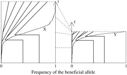
Figure 1.—

(A) The coalescent for the neutral locus is generated conditioned on the frequency X of the beneficial allele. (B) The time change dτ = (1 − X_t)dt transforms the process X to a supercritical branching process. The coalescent is also time changed. See text for explanation.

MODELS AND METHODS

Consider a population of N haploid individuals and two linked loci, a selected one and a neutral one. At the selected locus there are two alleles, a beneficial one and the wild type. The selected allele has a selective advantage of s compared to the wild type.

We study the selective phase of evolution by sampling at the end of a selective sweep. At the selected locus the founder of the selective sweep is an ancestor of all individuals in the sample. In contrast, the linked neutral loci are clustered into families that are identical by descent from the time the beneficial allele entered the population.

The Wright–Fisher model:

The benchmark to which we compare our approximations is a standard Wright–Fisher model with selection and recombination and model parameters (e.g., N = 10⁵ and s between 0.005 and 0.1) whose order of magnitude seems appropriate for certain real populations, e.g., Drosophila.

Simulations consist of a forward and a backward phase: first we generate the frequency path of a population that evolves according to the Wright–Fisher dynamics under selection forward in time. The starting frequency of the selected allele is 1/N. Denote by X_t the frequency of the beneficial allele in generation t. Conditioned on X_t−1, the number of beneficial alleles at time t is binomially distributed with parameters N and

(1)

If X eventually hits 1, we have generated a frequency path conditioned on fixation; otherwise, i.e., if X hits zero, we restart it from 1/N. We note that a Wright–Fisher path conditioned on fixation could in principle be simulated using transition probabilities for the frequencies of the beneficial allele that are conditioned to reach 1. These transition probabilities can be expressed in terms of the fixation probabilities, which, however, are known only approximately (Bürger and Ewens 1995). Since we want to use the Wright–Fisher model as an exact benchmark, we refrain from using this approximation here.

In the backward phase we take a sample of size n at the (random) time of fixation, which we trace back in time conditioned on the frequency path generated in the forward phase. Initially (i.e., at the end of the selective sweep forward in time) all lineages are linked to the advantageous allele. As the process moves from generation t to t − 1 (note that time t is measured forward), a lineage linked to a beneficial allele changes to a wild-type allele with probability r(1 − X_t−1), where r is the probability of recombination in one generation. Similarly, a lineage linked to the wild-type allele changes to the beneficial background with probability rX_t−1.

In addition, all lineages that are in the beneficial background choose their parents among all NX_t−1 individuals in generation t − 1. This determines the number of coalescences that occur. Similarly, the lineages in the wild-type background may also coalesce. Observe that this implies that an arbitrary number of coalescences in each time step may occur.

For large N, time measured in N generations and in the scaling α = sN, the Wright–Fisher model has a diffusion limit. In this limit the frequency path of the beneficial allele becomes the solution of the stochastic differential equation

(2)

where W denotes a Brownian motion. [This uniquely defines a diffusion with infinitesimal mean μ = αx(1 − x) and infinitesimal variance σ² = x(1 − x).] Conditioned on the fixation of X we can study the coalescent for a linked neutral variant backward in time using (2). In this coalescent each pair of lineages carrying the beneficial allele coalesces with rate at time t and each lineage changes from the beneficial to the wild-type background with rate ρ(1 − X_t), where ρ = rN is the scaled recombination rate (Kaplan et al. 1989).

We focus on two approximations of the Wright–Fisher model or its diffusion limit. The first is the logistic model, and the second is the Yule approximation.

The logistic approximation:

The structured coalescent process in a logistic background, which we simply call the logistic model, was introduced in Kaplan et al. (1989). It has been implemented since then in a number of programs for simulating selective sweeps (Braverman et al. 1995; Kim and Stephan 2002; Przeworski 2002; Li and Stephan 2005).

The logistic model relies on the assumption that genetic drift is negligible under strong selection. The frequency path of the beneficial allele is modeled by the logistic growth curve

(3)

which is (2) without genetic drift. Kaplan et al. (1989) consider a time-continuous version of the structured coalescent, but conditioned on the deterministic logistic frequency path given by (3), to describe the hitchhiking effect. As time is continuous in the logistic model, it is appropriate to specify rates at which events happen. Lineages at the neutral locus coalesce at time t with rate 1/X_t in the beneficial background and with rate 1/(1 − X_t) in the wild-type background. Any lineage at time t switches background from the beneficial to the wild type (backward in time) with rate r(1 − X_t) and from the wild type to the beneficial with rate rX_t.

To obtain positive frequencies in (3) the initial value X(0) =: ɛ must be >0. Various values of ɛ appear in the literature. Using α = sN as the scaled selection coefficient, Kaplan et al. (1989) and Braverman et al. (1995) suggest as a rule of thumb, while Stephan et al. (1992) as well as Przeworski (2002) use . In the logistic model, sample lineages that are in the beneficial background at time t = 0 are forced to coalesce immediately. This is the approach implemented in the above-mentioned programs for simulating selective sweeps. For more details on our implementation of the logistic approximation see the appendix.

The Yule approximation:

In recent mathematical studies (Schweinsberg and Durrett 2005; Etheridge et al. 2006) genealogies under hitchhiking have been approximated by a Yule process. This is a pure birth process in which lines independently split into two with rate α (Athreya and Ney 1972). The genealogical tree arising in this way is called a Yule tree.

We start off with a short description of the Yule process approximation: for large α, the random tree that arises by stopping the Yule process as soon as it reaches level ⌊2α⌋ proves to be a good approximation of the genealogy at the selective locus. A lineage at the neutral locus, traced back from the end of the sweep, is linked to its companion lineage at the selective locus. Recombination events separating the neutral from the beneficial locus in the Yule tree appear with a constant rate.

An essential step in the approximation is to ignore (i) back-recombinations from the wild-type to the beneficial background and (ii) coalescences in the wild-type background. An intuitive reason for this is that, viewed backward in time, recombination becomes effective only as long as the frequency X is low. Consequently lines may be found in the wild-type background only if X is low, which implies that the rate ρX for back-recombinations as well as the rate 1/(1 − X) for coalescences in the wild-type background is low. A mathematical justification of the approximation neglecting events in the wild-type background and an analysis of the order of convergence of the various error terms has been given in Schweinsberg and Durrett (2005) and Etheridge et al. (2006) and is complemented by numerical studies in this article.

A big conceptual and algorithmic advantage of this approximation is that it allows us to describe the genealogy at the neutral locus by a tree marked by points (recombination events) along its branches rather than a coalescent that is conditioned on a (random) frequency path of the beneficial allele. In the Yule process approximation, two individuals in the sample (two leaves of the tree) are identical by descent at the neutral locus from the beginning of the sweep if and only if they are not separated by a recombination event along their lineages.

This simple scheme of generating a genealogy under a selective sweep is based on the time transformation dτ = (1 − X_t)dt (see Figure 1). It takes the frequency path X from (2) into a stochastic process Y_τ = X_t that follows the stochastic dynamics

(4)

where is again a Brownian motion. The relation Y_τ = X_t is valid until Y hits frequency 1. The process Y given by (4) is known as a continuous-state branching process (Athreya and Ney 1972). It is the diffusion approximation of a supercritical Galton–Watson process in which, at times , a line splits in two lines with probability (1 + s)/2 and dies with probability (1 − s)/2. Once born, a line behaves independently from all other lines present.

Every birth in such a supercritical branching process has an infinite line of descent with probability 2s (Athreya and Ney 1972). Using this result, the genealogy of the infinite lines of descent in the diffusion approximation was established by O'Connell (1993) and Evans and O'Connell (1994). Viewed forward in time, this is a Yule process with parameter α, i.e., a pure birth process in which every line splits in two lines with rate α. [This process was originally invented by the Scottish scientist and statistician Udny Yule (1871–1951) to study the evolution of species (Yule 1924).] When the Yule process has i lines, the process Y has frequency

(5)

in expectation. Thus, when Y reaches frequency 1, the Yule process has 2Ns = 2α lines. To approximate the time-changed genealogy at the selective locus, we thus use the Yule process stopped when it has ⌊2α⌋ lines.

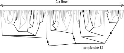
The genealogy of a sample at the selective locus appears as a subtree of this Yule tree; see Figure 2. On this subtree, recombination events along the sample genealogy are marked by solid circles. In this example, the sample is partitioned into four families of sizes 4, 2, 4, and 2, respectively.

Figure 2.—

A Yule tree approximating the genealogy of a selective sweep. The thick lines represent the genealogy of the sample; solid circles correspond to recombination events along the branches. See text for explanation.

Next, we describe how the sample's approximate genealogy is extracted from the Yule tree. By the time transformation the coalescence rate of a pair of lineages changes from 1/Xdt to 1/(Y(1 − Y)) dτ, see Figure 1. As a consequence, if there are k lineages left in the sample genealogy and the Yule tree has i lineages, then using (5), the rate at which k decreases to k − 1 is

(6)

Since the Yule tree shrinks from i to i − 1 lineages with rate iα, this suggests to embed the sample genealogy at the selective locus into the Yule tree backward in time as follows: when the Yule tree goes from i to i − 1 lineages, a pair of the sample lineages coalesces with probability

(7)

Since the time transformation changes the recombination rate from ρ(1 − X)dt to , the recombination events are mapped on the Yule tree in a particularly simple way, making it easy to generate recombination events along the lineages: consider a branch between the times when the Yule tree has i₁ and i₂ lines. The time interval when the Yule tree has i lines is exponentially distributed with rate iα. As recombination events occur at constant rate ρ, the probability that no recombination event hits the branch is

(8)

the approximation being accurate if or more precisely if r/s is of the order 1/log(Ns) (Etheridge et al. 2006). The Yule approximation thus allows us to simulate the random partition of a sample (with respect to identity by descent at the neutral locus) in two stages: first, generate the sample genealogy by the coalescence mechanism (7), and then generate recombination events along the sample lineages with probabilities (8). Note that this method does not require any explicit simulation of the frequency curve X or that of the full Yule tree. A thorough description of the implementation of the Yule process approximation is given in the appendix.

Connections with previous work:

A precursor of the Yule approximation described above was introduced in a diffusion setting by Etheridge et al. (2006). It generates the same genealogies as the Yule approximation given by Schweinsberg and Durrett (2005) for the Moran model. The modification we make here deals with the way to extract the sample tree out of the Yule tree. In Schweinsberg and Durrett (2005) and Etheridge et al. (2006) the pair coalescence probability for k sample lineages when the Yule tree has i lines is , which corresponds to absence of the factor (1 − Y) in (6).

We included neither the procedure for taking a sample out of the full Yule tree that ignores the factor (1 − Y) nor the approximate sampling formula from Etheridge et al. (2006) into our numerical studies. The reason is that these approaches produce accurate results only for small samples; i.e., n ≤ 5 (results not shown). For the special case of n = 2 in a Moran model, simulation studies by Schweinsberg and Durrett (2005) already showed that the Yule approximation outperforms the logistic one.

RESULTS

Using simulations for data analysis requires accurate and fast algorithms. Although the simulation of the coalescent for the Wright–Fisher model is still much faster compared to forward simulations of the whole population, it is much slower compared to the logistic (e.g., a factor 200 for N = 10⁵, s = 0.01, r = 0.001, n = 12) and the Yule (a factor 1000 for the same parameters) approximations. It becomes especially slow for large populations.

The need for approximations leads directly to the question of which approximation to use. The logistic approximation is appealing because it is exact except for the deterministic frequency path. This approximation seems reasonable for strong selection. The Yule approximation has the advantage that no simulation of a frequency path is necessary; in fact, this approximation arose through an averaging over the frequency paths. Moreover, it can be implemented with no more effort than the logistic model (see Algorithm 2 in the appendix).

Both accuracy and speed are necessary for the quality of an approximation. The speed for the two approximations is comparable for relevant parameter ranges, e.g., α < 4000, n = 12. The accuracy of the Yule approximation turns out to be better than that of the logistic model. However, in both approximations the error is small, e.g., for the distribution of Tajima's D or for a maximum-likelihood estimator of the position of the selective locus in the genome.

Our simulation results are shown in the following sections. First we comment on the speed of both approximations. Then we proceed with an analysis of relevant parameter ranges where we also derive a prediction for the reduction in heterozygosity from the Yule approximation. Afterward, the analysis of the quality of the logistic and Yule approximations is carried out. Recall that the Yule approximation neglects events that happen in the wild-type background. We check numerically for which parameter ranges this particular approximation step is justified. Then we compare the error of the Yule and the logistic approximations, and finally we test how big the error is in applications.

Run times:

For the logistic model, we follow the algorithm from Braverman et al. (1995) and Kim and Stephan (2002) and discretize the logistic growth curve into 1000 intervals. The Yule approximation has been described above. As this process stops when the Yule tree has ⌊2α⌋ lines, run times increase with α. The run time of the logistic model does not depend on α.

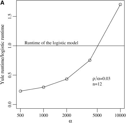
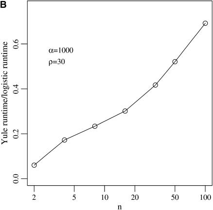
For N = 10⁵ and s = 0.01 the simulations using a Wright–Fisher model are 200 times slower than the logistic approximations. Figure 3 illustrates the difference in speed for the two approximations.

Figure 3.—

Run-time ratios for simulating the logistic and Yule approximations. Run time depends on (A) the selection strength α and (B) the sample size n.

Parameter ranges:

Usually a reduction in heterozygosity is used to infer strong directional selection. We therefore investigate which parameter combinations of N, s, and r lead to a significant reduction in variation. As a selective sweep is very short, it is unlikely that two lineages would coalesce in that time under neutral evolution. However, by directional selection, the chance of coalescence in the sweep increases as the recombination distance to the selected site decreases. We look at the probability h of coalescence of two lineages in the sweep as a measure of the strength of selection. As Stephan et al. (1992) observe, h equals the factor by which the expected heterozygosity at linked neutral sites during the selective sweep is reduced.

Apart from simulating the Wright–Fisher model to approximate h, known approximations to the probability of coalescence in the sweep can be derived by (i) direct simulation or computation in the logistic model or (ii) the Yule approximation. In the logistic model such approximations have been obtained in Equation 19 of Stephan et al. (1992) (see also Wiehe and Stephan 1993, Equation 1b). In the Yule approximation there is a random number J of lineages in the Yule tree at the time when the two sample lineages coalesce. The probability of coalescence within k sample lineages at the time when the full Yule tree goes from i to i − 1 lineages is given by (6); we can therefore calculate for k = 2

A sample of two lineages at a neutral locus linked to the selected one shares the history of the corresponding lineages at the selected locus if no recombination occurs. To a good approximation, if recombination pushes one of the two lineages out of the beneficial background, the two neutral lineages are not identical by descent at the beginning of the sweep.

Therefore, given J = j, the two lineages at the neutral locus coalesce during the sweep if no recombination occurs on either branch leading from j to ⌊2α⌋. The probability that no recombination event falls on a branch was given in Equation 8. So

This is the approximation of h based on the Yule model.

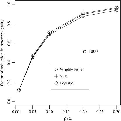
Figure 4 shows that the analytic formulas for the reduction of heterozygosity obtained from the logistic and Yule approximations are numerically sound. Additionally, we can read parameter ranges for r and s where the hitchhiking effect determines patterns of sequence diversity. Hitchhiking cannot be observed if the reduction in sequence variation is too low. For r/s = ρ/α = 0.1, the factor by which heterozygosity is reduced is as high as 0.7. This is reflected in simulations carried out by Fay and Wu (2000), who showed that neutrality tests can detect a recent selective sweep only as long as ρ/α < 0.1. In other words, selection intensity has to be one order of magnitude larger than recombination to detect a hitchhiking effect. This agrees with the condition that recombination is weaker than selection by a factor of log α that was used by Etheridge et al. (2006) in a theoretical study of the Yule approximation. Our results show that in this regime (and for moderate sample sizes n) the Yule approximation becomes accurate for large α also from a practical point of view. If one wants to go beyond this regime, say to recombination rates that are of the same order of magnitude as the selection strength, back-recombinations into the favorable background cannot be neglected any more. Back-recombinations could be incorporated by another refinement of the Yule approximation: one can estimate the back-recombination rate ρX_t dt = ρY_τ/(1 − Y_τ)dτ from the current state i of the Yule process in the same manner as the coalescence rate was estimated in Equation 6. In this study, we do not pursue this further. Instead, we show in the next section that for the regime ρ/α < 0.1, and for a moderate sample size n = 12, it is indeed justified to neglect the events in the wild-type background.

Figure 4.—

Heterozygosity is reduced by a factor h depending on the selection strength, α, and the recombination rate, ρ, during a selective sweep. Both theoretical predictions for the logistic and Yule model work well.

Events in the wild-type background:

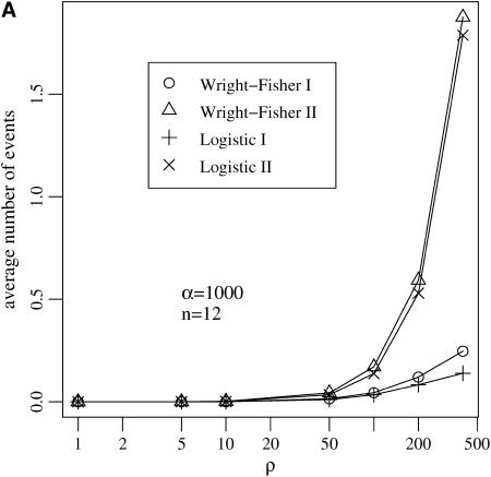
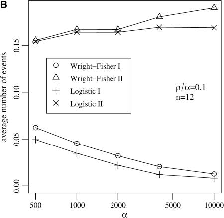
Several assumptions underlie the Yule approximation of a selective sweep. We argued that both coalescences in the wild-type background and back-recombinations into the beneficial background occur with negligible probability. These events are excluded in the Yule approximation. This is in contrast to the logistic model by Kaplan et al. (1989), which allows for events in the wild-type background. As Figure 5 shows, the assumptions that none of these events happen in the wild-type background is reasonable, at least for a wide range of parameters.

Figure 5.—

Two kinds of events may occur backward in time in the genealogy of the linked neutral variant in the wild-type background: (I) coalescence events and (II) recombinations with a beneficial allele denoted by back-recombinations. (A) The average number of these events increases with the recombination rate ρ, but (B) for fixed ρ/α stays bounded for a wide range of values of the selection strength α. The Yule approximation does not allow for any of these events.

In the wild-type background the average number of back-recombinations is larger than the number of coalescence events. The number of back-recombinations rapidly increases for ρ > 0.1α (see Figure 5A). For such parameter combinations the reduction in heterozygosity is low and a selective sweep does not leave a distinct footprint (Figure 4). If ρ/α ≤ 0.1, the average number of events in the wild-type background never exceeds 0.2 in a sample of size 12 (Figure 5B). In all cases, the logistic model approximates the Wright–Fisher model well.

Comparing the approximation error:

To check how close the approximations are to the Wright–Fisher model, we need quantitative measures. For our sample, two factors determine the shape of sequence diversity: first, the times of coalescence and second, which pairs of lines coalesce. As a selective sweep is short compared to the neutral expectation of time of coalescence of two lines, only the latter quantity determines observable diversity patterns.

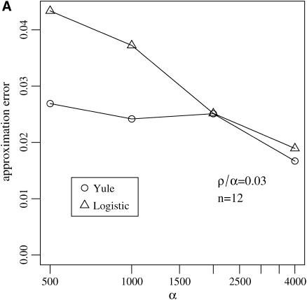
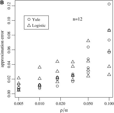
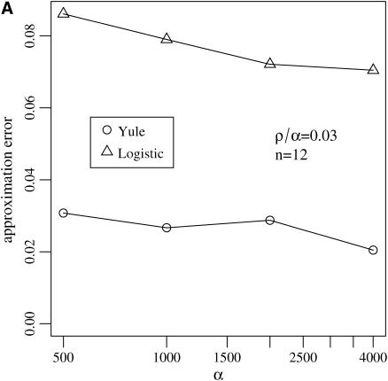
Identity by descent partitions the n lineages into families with a common ancestor at the beginning of the sweep. We study two statistics in our simulations that are related to this concept. First, we check whether the distribution of the sizes of the largest and the second-largest families are approximated well; second, we study the distribution of the number of lineages that trace back to the founder of the selective sweep and the size of the largest recombinant family. It turns out that the Yule approximation is superior to the logistic approximation in both cases (see Figures 6 and 7).

Figure 6.—

Approximation errors and for the sizes of the two biggest families that are identical by descent during the sweep for the Yule and the logistic models. Every point is based on 10⁵ simulations of a sample of size 12 in the Wright–Fisher model with population size 10⁵ and the corresponding approximating Yule and logistic models. (A) The ratio of recombination rate and selection strength ρ/α = 0.03 is fixed and α varies. (B) Several ratios ρ/α were considered. For each of these ratios, α = 500, 1000, 2000, and 4000 are considered. The values for ρ/α = 0.03 are based on the simulations shown in A.

Figure 7.—

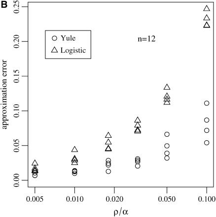
Approximation errors and for the number of lineages going back to the founder of the sweep and the size of the largest recombinant family for the Yule and the logistic models. The same simulations and parameter combinations as in Figure 6 were used.

We perform simulations to follow n = 12 lineages back during the sweep. A special role is played by the founder of the sweep. Lineages that are not hit by a recombination event during the sweep descend from the founder of the sweep. Conversely, all lineages that do not trace back to the founder of the sweep must have been hit by a recombination event. However, these lineages may still have coalesced and thus be identical by descent from the beginning of the sweep. So identity by descent gives (i) the number of lineages that trace back to the founder of the sweep and (ii) sizes of recombinant families that trace back to individuals in the wild-type background. We define

and

We compute the error in the approximations compared to the Wright–Fisher model for the distribution of pairs (F₁, F₂) as well as (F′₁, F′₂). By this we mean the following: probabilities P[F₁ = f₁, F₂ = f₂] are approximated in the Wright–Fisher model by the Monte Carlo estimates

Analogously we may use our approximations and obtain estimates and for the Yule approximation and the logistic approximation. Then consider the errors

(9)

where □ is Y or L, standing for either the Yule or the logistic approximation. We consider only two random variables simultaneously (i.e., either F₁ and F₂ or F′₁ and F′₂) because of limitations of computational power. The outcomes for fixed and variable ρ/α are illustrated in Figures 6 and 7 for , and , , respectively.

For the approximation errors and the Yule model performs slightly better than the logistic model for a wide range of parameters. Indeed, the frequencies of the two largest families that are identical by descent are better approximated by the Yule model as can be seen from Figure 6. In the case of ρ/α = 0.03, only for selection strengths α > 2000 does the logistic model have an approximation error similar to the Yule approximation. For larger recombination rates, i.e., ρ/α ≥ 0.05, the Yule approximation becomes worse. For values α > 4000 and N = 10⁵, the diffusion process (2) is not a good approximation of the Wright–Fisher model, which assumes a scaling with α of the order of 1. For larger populations the diffusion approximation works better. However, we did not pursue the study for larger populations because run times for the Wright–Fisher model increase linearly with population size.

As far as the distribution of the number of lineages that go back to the founder of the sweep and the size of the largest recombinant family is concerned, the quality of the logistic model deteriorates. A comparison of and shows that the approximation error of the Yule model is half the size of the error introduced by the logistic model. Figure 7 illustrates this situation.

While errors for the Yule approximation and are almost the same, this is not true for the logistic model. The values of are more than twice as large as the values of .

The approximation error in applications:

Any approximation, be it of the logistic or the Yule type, introduces some error into simulations. For practical purposes, however, it is not clear which amount of approximation error materially affects the analysis of real data.

The coalescent is successful in modern analysis of sequence polymorphisms because it stores all information inherent in the observed data. So far, we discussed a phase in the evolution of a population only where strong positive selection was acting. Assume now that the population was in equilibrium when the beneficial allele first appeared. For the coalescent this implies that we add to the coalescent obtained under strong selection during the sweep a neutral coalescent before the beginning of the sweep. So we simulate both the coalescent under hitchhiking, where some lineages have already coalesced, and the neutral phase, where the rest of the lineages coalesce. Here coalescence occurs with rate when currently k lineages are present. Neutral mutations are added to this tree using a Poisson process with rate θ/2.

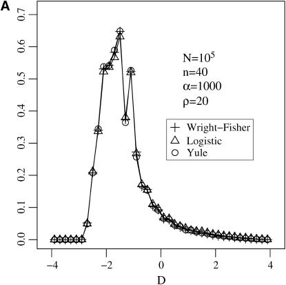
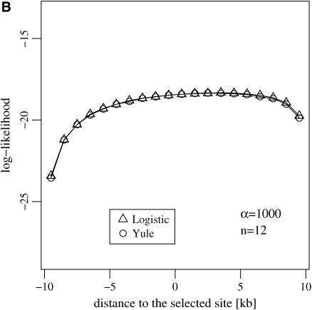
We now study the errors induced by applying the approximations to (i) the distribution of Tajima's D (Tajima 1989) and (ii) the likelihood curve for the target of selection in a genome (see Figure 8). We find that both approximations are numerically sound.

Figure 8.—

(A) The distribution of Tajima's D estimated at the end of a selective sweep by simulating the Wright–Fisher model and the logistic and the Yule approximations during the selective phase. (B) The log-likelihood curve for the position of a selected locus given data from two adjacent neutral loci. The position of the selected site is at 0.

The likelihood curve of the target of selection in a genome is obtained in the following situation: sequence data are available from two neutral loci flanking a selected locus. The aim is to estimate the position of the selected locus by drawing its likelihood curve. This can be done under the assumption that the selection strength and per site recombination rates are known and that data from both neutral sites are independent. This is reasonable because it was shown in Stephan et al. (2006) that linkage disequilibrium vanishes for sites on different sides of a selected locus at the end of the sweep. As data from the two loci we consider the compact frequency spectrum; i.e., we record the number of SNPs that are singletons, doubletons, and all the others (see, e.g., Li and Stephan 2005). So our data consist of six numbers, three for each neutral locus.

The likelihood curve is found by simulation, either with a logistic or with a Yule approximation. The result, given in Figure 8, shows that both approximations produce equal results.

DISCUSSION

The concept of genetic hitchhiking, or selective sweeps, which goes back to Maynard Smith and Haigh (1974), has become important for the interpretation of DNA sequence data. Above all, selective sweeps help to find genes under strong positive selection that are important for an adaptive process (see, e.g., Sabeti et al. 2002 and Beisswanger et al. 2006). We compared two approximate models for genetic hitchhiking, the logistic and the Yule model. Specifically, we tested by simulation which of the two is more appropriate in terms of its fit to the Wright–Fisher model with selection and recombination.

The logistic model relies on the approximation that genetic drift can be ignored under strong selection. This approximation is useful for the theoretical understanding of genetic hitchhiking (Kaplan et al. 1989; Stephan et al. 1992). Its analysis has recently been extended to study two neutral loci linked to the selected site to predict patterns of linkage disequilibrium (Stephan et al. 2006).

The Yule approximation relates selective sweeps with supercritical branching processes. Already Fisher (1930) observed that the frequency path of a beneficial allele that enters a population may be approximated by a supercritical branching process. This insight was applied to selective sweeps by Barton (1998) who argued that the approximation of the frequency path of a strongly beneficial allele works only as long as its frequency exceeds a certain threshold. And, in fact, his study uses a supercritical branching process with supercriticality 2s as an approximation of the early phase of a selective sweep.

To study the selective sweep from start to finish using a supercritical branching process we use the time transformation (4). By this transformation we obtain a one-to-one correspondence between the paths of the Wright–Fisher diffusion with selection (2) and supercritical branching processes. This time transform works until the branching process hits frequency 1, where it is stopped.

Since Kaplan et al. (1989), the genealogy of a sample of neutral loci linked to a selected locus has been studied using a structured coalescent. The structure is given by the beneficial and the wild-type background and the change in background is due to recombination between the neutral and the selected locus.

The structured coalescent can also be studied for stochastically fluctuating frequencies given by (2); equivalently, using the one-to-one correspondence to supercritical branching processes, we may as well consider frequencies given by the Feller branching diffusion (4). The reason why supercritical branching processes are easy to handle is that their genealogies are explicit. This applies in particular to the lines of infinite descent, which form a Yule process. For the genealogy at the neutral locus linked to the selected one, recombination events can be represented as marks on the branches of the Yule tree occurring with constant rate (Etheridge et al. 2006).

There are two reasons why the Yule process we consider is only an approximation to a selective sweep. First, the time transform given above deals with diffusion limits rather than finite populations. However, in a setting using the Moran model the Yule process was shown to be a valid approximation (Schweinsberg and Durrett 2005). Second, the Yule tree produces the genealogy only at the selected site and hence, events in the wild-type background cannot be mapped onto this tree. Fortunately, these events are rare. This was shown by the approximate result in Schweinsberg and Durrett (2005) and Etheridge et al. (2006) as long as (ρ/α)² is small and is also confirmed by our simulations. For parameter ranges where the reduction in variation is still strong in a sample of size n = 12 (meaning, e.g., that the heterozygosity is reduced by at least 30% or ρ/α < 0.1) these events can safely be ignored. Less than 0.2 such events occur during a sweep with α ranging between 500 and 10,000 (see Figure 5). This might change for larger samples, as was, e.g., considered in Barton (1998) because the reduction in variation might still be high in parameter ranges where back-recombinations are frequent. For n = 12, we also see that the number of back-recombinations increases drastically for ρ/α ≥ 0.1. In this parameter regime, lines are jumping back and forth between the beneficial and the wild-type background, but as back-recombinations become less probable toward the beginning of the sweep many will end up in the wild-type background at the beginning of the sweep.

We check and compare the quality of the logistic model and the Yule approximation by a simulation study. The parameter ranges we use are chosen such that the standard assumptions of genetic hitchhiking are met; in addition, they should lead to observable patterns in sequence data. By this we mean that , so that we can expect a strong reduction in diversity, and to ensure that the neutral locus is in the valley of reduction of variation. In our studies we picked a moderate sample size of n = 12. The population size enters into the simulation of the logistic and Yule approximation only by the factor α = Ns and the scaled recombination rate. However, for fixed α, the run time of the Wright–Fisher model is approximately linear in N and becomes too slow to produce enough iterations if N > 10⁶.

Both the logistic and the Yule approximations are fast. However, the speed of the two procedures is controlled by different mechanisms. For the logistic model, the speed is mostly dependent on the number of time steps simulated during the selective sweep. We follow the algorithm of Kim and Stephan (2002) and use 1000 such steps. The speed of the Yule approximation depends on 2α, as the Yule tree is stopped upon reaching ⌊2α⌋ lines. Comparing both models with 1000 discretization steps, i.e., α = 500, the Yule approximation is faster by a factor of 4 in a sample of size 12 (see Figure 3).

To test for the quality of the approximation we used two different measures. The first is identity by descent of the lineages in the sample at the beginning of the selective sweep; these are measured by and as given by (9) for the logistic and the Yule approximations, respectively. The second is the number of lineages that trace back to the founder of the sweep and the size of the largest recombinant family, given by and , respectively.

Part of the error in the Yule approximation comes from neglecting events in the wild-type background. As the logistic model accounts for these events as well and gives good estimates for their number, it has advantages in this respect. However, the Yule model gives a better approximation for identity by descent over a wide range of parameters in spite of ignoring the events in the wild-type background. Only for large values of s and ratios r/s > 0.05 is the logistic model superior. Hence, we conclude that the Yule approximation gives a significantly better approximation for events in the beneficial background than the logistic model.

The logistic approximation does not take into account fluctuations in the frequency of the beneficial allele in the early phase of a selective sweep. As a consequence, it produces incorrect estimates for the occurrence of events in that phase. This is seen in our simulations from the fact that the number of lineages that trace back to the founder of the sweep is estimated less accurately than identity by descent from the beginning of the sweep. We find that the approximation error produced by the logistic model is twice as large as the corresponding measure for the Yule approximation over all parameters considered.

Consider, e.g., statistics like the frequency of the major haplotype, the frequency distribution obtained from a sample, Tajima's D, or the likelihood curve of the target of selection if data from two neutral loci are given. The distribution of these statistics can be predicted/simulated under hitchhiking once the distribution of the genealogy of the sample is known approximately; it is mostly controlled through identity by descent from the beginning of the sweep. Thus, it is not too surprising that both the simulated distribution of Tajima's D and the likelihood curve for the target of selection produce good results for both the logistic and the Yule approximations.

Not only does the Yule approximation give accurate results in simulations, but also it has proved to be useful in the analytical understanding of patterns of genealogies at neutral sites linked to a strongly beneficial one (Durrett and Schweinsberg 2005; Etheridge et al. 2006). These analytical results cover the estimated decrease in heterozygosity and the probability that a lineage escapes the sweep as well as an approximate sampling formula under genetic hitchhiking and results for a recurring sweep model.

There is justified hope that the Yule approximation may also lead to a deeper understanding of further questions related to hitchhiking. These might include: genealogical trees for a model of overlapping selective sweeps, selective sweeps in structured populations, or the analysis of soft sweeps (Hermisson and Pennings 2005). In addition, an extension of the Yule model to several loci is feasible (P. Pfaffelhuber and A. Studeny, unpublished results). Here, taking multiple neutral loci into account, one has to study the ancestral recombination graph conditioned on the frequency path X. Lines may not only coalesce and change their background but also split in either background. As the period where splits in the beneficial background occur is separated in time from both recombinations with wild-type individuals and coalescence events these can be generated independently from the rest of the genealogy.

The Yule approximation in its present forms also has drawbacks. Events in the wild-type background are ignored, which leads to approximation errors for r/s > 0.1. However, back-recombinations as well coalescence events can be incorporated into the Yule process. This could be done by estimating Y from the number of lines in the Yule process by the same procedure that leads to (6).

Another drawback of the Yule approximation is that only one neutral locus linked to a selected one is implemented and analyzed numerically. However, genome scans, which are used to find targets of selection, produce multilocus data (see, e.g., Glinka et al. 2003). In addition, statistical tests based on a full-likelihood analysis such as those by Li and Stephan (2005) rely on multilocus simulations of hitchhiking and therefore cannot yet be treated by the Yule process. However, composite-likelihood approaches such as those given in Kim and Stephan (2002) treat different loci as unlinked, which makes it possible to use the Yule approximation here. Multilocus extensions not only allow for more applications in simulating selective sweeps, but also direct the way to theoretical predictions for measures of linkage disequilibrium under hitchhiking, which were started in Stephan et al. (2006).

A further application of the Yule process approximation could be to develop methods in the spirit of Griffiths and Tavare (1994), Stephens and Donnelly (2000), Fearnhead and Donnelly (2001), and De Iorio and Griffiths (2004), which work in the presence of strong selection and recombination. Here, the Yule process approximation should help to obtain proposal distributions for importance sampling of genealogies conditioned under sequence data that arose by neutral mutation and genetic drift, followed by a loss of diversity due to a selective sweep.

APPENDIX: IMPLEMENTATION OF THE APPROXIMATIONS

The logistic model was implemented using the algorithm given by Braverman et al. (1995) and Kim and Stephan (2002) as implemented in the program ssw by Yuseob Kim. The coalescence and recombination events were simulated using a step function instead of the logistic sweep curve. We followed the common practice suggested by Kaplan et al. (1989) and Braverman et al. (1995), that the frequency path should be started with a frequency and end with frequency 1 − ɛ. However, our conclusions are not affected by the choice of ɛ (results not shown). Lineages in the beneficial background at the beginning of the sweep were forced to coalesce.

We follow Kim and Stephan (2002) and discretize the selective sweep into 1000 time steps with a step function rather than a smooth curve as the frequency curve of the beneficial allele. Tracing the ancestry backward in time, we have to wait a random amount of time until the next event in the coalescent happens.

The probabilities that an event happens in time dt can be given explicitly; see, e.g., Braverman et al. (1995). We use Algorithm 1 to generate these events. Observe that time is running backward. The numbers p₁, p₂, p₃, …, are the probabilities that the next event occurs in the first, second, etc., discretization step of the sweep (backward in time). Assume that we already know all events up to time j. Set i to the current time, pick a random number x that is uniformly distributed on [0, 1], and set p = 0. During the algorithm p increases; in particular, in the ith step, p is the probability that the event occurs after at most i steps. So the number of steps we need for p ≥ x will be the number of steps until the next event.

By this approach we have to draw as many random numbers as there are events during the sweep. Observe that Algorithm 1 certainly terminates in our special case because it automatically ends after 1000 time steps by setting p₁₀₀₀ = 1.

• Algorithm 1: How to sample from the waiting time until the next event:

• Require: p_i, i = 1, 2, …, {probabilities that an event happens in the ith step}

• Require: j {starting index}

•  , ,

•  while p < x do

•   

•   

• output i.

How the Yule approximation is implemented can be read from the pseudocode given in Algorithm 2. Recall that a tree can conveniently be stored as an array of nodes. A node has a time coordinate as well as coordinates indicating the ancestor and children. Binary trees have 2n − 1 nodes, so the array tree has length 2n − 1. The first n positions in the array encode the leaves of the genealogical tree. The tree itself gives the genealogy at the selected site. The tree topology arises by coalescing two lineages at random. For this, a list of active nodes (live) is created, starting with all leaves of the tree. When two nodes coalesce, they are removed from live and replaced by their ancestor. The times of the nodes represent the number of lines in the full Yule tree; e.g., all leaves have time 2α, as the Yule tree is stopped upon reaching 2α lines. Generating the times of coalescence events is done using Algorithm 1. The probability of coalescence in step i is given by (6). As explained above, the neutral genealogy can be generated by marking the Yule tree with a constant rate. This can be done using the probabilities (8). Two nodes not separated by a recombination event are identical by descent from the beginning of the sweep.

• Algorithm 2: Yule approximation to hitchhiking:

• Require: tree {array of 2n − 1 nodes, first n are leaves, the others are internal nodes}

• Require: time {array of times of 2n − 1 nodes}

• Require: hit {array of 0/1's, 1 indicates that the lineage to a node is hit by a recombination event}

•  {Initializing nodes}

•  for all 0 ≤ i < 2n − 1 do

•    {the Yule process is stopped with ⌊2α⌋leaves}

•  {Generating the tree topology}

•  

•  for all n ≤ i < 2n − 1 do

•   pick two elements tree_j and tree_k from live at random

•   ancestor of tree_j and tree_k is tree_i

•   remove tree_j, tree_k from live, add tree_i to live

•  {Generating times for the nodes of the sample}

•  

•  while k > 1 do

•   {Now, use Algorithm 1 with probabilities , p_j−1^k, …, from (7) and j to create the next waiting time}

•   

•   

•   

•  {Throwing recombinations on the tree}

•  for all 0 ≤ i < 2n − 2 do

•   

•   

•   mark the branch from node i to its ancestor with probability from (8).

The program HITCHHIKING that we developed for our numerical studies implements all three models. It can be downloaded at http://adenine.biz.fh-weihenstephan.de/hitchhiking.

References

- Athreya, K., and P. Ney, 1972. Branching Processes. Springer, Berlin.
- Barton, N., 1998. The effect of hitch-hiking on neutral genealogies. Genet. Res. 72: 123–133. [Google Scholar]
- Beisswanger, S., W. Stephan and D. DeLorenzo, 2006. Evidence for a selective sweep in the wapl region of Drosophila melanogaster. Genetics 172: 265–274. [DOI] [PMC free article] [PubMed] [Google Scholar]
- Braverman, J., R. Hudson, N. Kaplan, C. Langley and W. Stephan, 1995. The hitchhiking effect on the site frequency spectrum of DNA polymorphism. Genetics 140: 783–796. [DOI] [PMC free article] [PubMed] [Google Scholar]
- Bürger, R., and W. J. Ewens, 1995. Fixation probabilities of additive alleles in diploid populations. J. Math. Biol. 33: 557–575. [Google Scholar]
- Coop, G., and R. Griffiths, 2004. Ancestral inference on gene trees under selection. Theor. Popul. Biol. 66: 219–232. [DOI] [PubMed] [Google Scholar]
- De Iorio, M., and R. C. Griffiths, 2004. Importance sampling on coalescent histories. Adv. Appl. Probab. 36: 417–433. [Google Scholar]
- Durrett, R., and J. Schweinsberg, 2004. Approximating selective sweeps. Theor. Popul. Biol. 66(2): 129–138. [DOI] [PubMed] [Google Scholar]
- Durrett, R., and J. Schweinsberg, 2005. A coalescent model for the effect of advantageous mutations on the genealogy of a population. Stoch. Proc. Appl. 115: 1628–1657. [Google Scholar]
- Etheridge, A., P. Pfaffelhuber and A. Wakolbinger, 2006. An approximate sampling formula under genetic hitchhiking. Ann. Appl. Probab. 16(2): 685–729. [Google Scholar]
- Evans, S. N., and N. O'Connell, 1994. Weighted occupation time for branching particle systems and a representation for the supercritical superprocess. Can. Math. Bull. 37(2): 187–196. [Google Scholar]
- Fay, J. C., and C.-I Wu, 2000. Hitchhiking under positive Darwinian selection. Genetics 155: 1405–1413. [DOI] [PMC free article] [PubMed] [Google Scholar]
- Fearnhead, P., and P. Donnelly, 2001. Estimating recombination rates from population genetic data. Genetics 159: 1299–1318. [DOI] [PMC free article] [PubMed] [Google Scholar]
- Fisher, R. A., 1930. The Genetical Theory of Natural Selection, Ed. 2. Clarendon Press, Oxford.
- Glinka, S., L. Ometto, S. Mousset, W. Stephan and D. De Lorenzo, 2003. Demography and natural selection have shaped genetic variation in Drosophila melanogaster: a multi-locus approach. Genetics 165: 1269–1278. [DOI] [PMC free article] [PubMed] [Google Scholar]
- Griffiths, R. C., and S. Tavare, 1994. Simulating probability distributions in the coalescent. Theor. Popul. Biol. 46: 131–159. [Google Scholar]
- Hermisson, J., and P. Pennings, 2005. Soft sweeps: molecular population genetics of adaptation from standing genetic variation. Genetics 169: 2335–2352. [DOI] [PMC free article] [PubMed] [Google Scholar]
- Kaplan, N. L., R. R. Hudson and C. H. Langley, 1989. The “hitchhiking effect” revisited. Genetics 123: 887–899. [DOI] [PMC free article] [PubMed] [Google Scholar]
- Kim, Y., and W. Stephan, 2002. Detecting a local signature of genetic hitchhiking along a recombining chromosome. Genetics 160: 765–777. [DOI] [PMC free article] [PubMed] [Google Scholar]
- Li, H., and W. Stephan, 2005. Maximum-likelihood methods for detecting recent positive selection and localizing the selected site in a genome. Genetics 171: 377–384. [DOI] [PMC free article] [PubMed] [Google Scholar]
- Maynard Smith, J., and J. Haigh, 1974. The hitch-hiking effect of a favorable gene. Genet. Res. 23: 23–35. [PubMed] [Google Scholar]
- Nurminsky, D., 2005. Selective Sweep. Kluwer, Dordrecht, The Netherlands/Norwell, MA.
- O'Connell, N., 1993. Yule process approximation for the skeleton of a branching process. J. Appl. Probab. 30: 725–729. [Google Scholar]
- Przeworski, M., 2002. The signature of positive selection at randomly chosen loci. Genetics 160: 1179–1189. [DOI] [PMC free article] [PubMed] [Google Scholar]
- Sabeti, P., D. Reich, J. Higgins, H. Levine, D. Richter et al., 2002. Detecting recent positive selection in the human genome from haplotype structure. Nature 419(6909): 832–837. [DOI] [PubMed] [Google Scholar]
- Schweinsberg, J., and R. Durrett, 2005. Random partitions approximating the coalescence of lineages during a selective sweep. Ann. Appl. Probab. 15: 1591–1651. [Google Scholar]
- Stephan, W., T. H. E. Wiehe and M. W. Lenz, 1992. The effect of strongly selected substitutions on neutral polymorphism: analytical results based on diffusion theory. Theor. Popul. Biol. 41: 237–254. [Google Scholar]
- Stephan, W., Y. Song and C. Langley, 2006. The hitchhiking effect on linkage disequilibrium between linked neutral loci. Genetics 172: 2647–2663. [DOI] [PMC free article] [PubMed] [Google Scholar]
- Stephens, M., and P. Donnelly, 2000. Inference in molecular population genetics. J. R. Stat. Soc. Ser. B 62: 605–655. [Google Scholar]
- Tajima, F., 1989. Statistical method for testing the neutral mutation hypothesis by DNA polymorphism. Genetics 123: 585–595. [DOI] [PMC free article] [PubMed] [Google Scholar]
- Wiehe, T., and W. Stephan, 1993. Analysis of a genetic hitchhiking model, and its application to DNA polymorphism data from Drosophila melanogaster. Mol. Biol. Evol. 10(4): 842–854. [DOI] [PubMed] [Google Scholar]
- Yule, G. U., 1924. A mathematical theory of evolution, based on the conclusion of Dr. J.C. Willis, F.R.S. Philos. Trans. R. Soc. Lond. Ser. B 213: 21–87. [Google Scholar]