Modeling Electroporation in a Single Cell

Abstract

Electroporation uses electric pulses to promote delivery of DNA and drugs into cells. This study presents a model of electroporation in a spherical cell exposed to an electric field. The model determines transmembrane potential, number of pores, and distribution of pore radii as functions of time and position on the cell surface. For a 1-ms, 40 kV/m pulse, electroporation consists of three stages: charging of the cell membrane (0–0.51 μs), creation of pores (0.51–1.43 μs), and evolution of pore radii (1.43 μs to 1 ms). This pulse creates ∼341,000 pores, of which 97.8% are small (≈1 nm radius) and 2.2% are large. The average radius of large pores is 22.8 ± 18.7 nm, although some pores grow to 419 nm. The highest pore density occurs on the depolarized and hyperpolarized poles but the largest pores are on the border of the electroporated regions of the cell. Despite their much smaller number, large pores comprise 95.3% of the total pore area and contribute 66% to the increased cell conductance. For stronger pulses, pore area and cell conductance increase, but these increases are due to the creation of small pores; the number and size of large pores do not increase.

INTRODUCTION

Electroporation is a technique that uses electric pulses to create transient pores in the cell membrane, which promote the delivery of biologically active molecules into cells (1–4). Despite great interest in this technique, its practical applications are hampered by the lack of a good understanding of the processes taking place during electroporation. Of particular interest is the electroporation process occurring in an isolated cell, since the vast majority of practical applications involve either cell suspensions, tissues composed of cells that are not connected by gap junctions, or, more recently, single cells in microfluidic devices. Hence, numerous studies use a variety of experimental techniques, such as uptake of fluorescent molecules (5,6), imaging of the cell's transmembrane potential (7), or measuring cell's impedance (8) to provide insight into cell electroporation. Nevertheless, some questions cannot be answered with available experimental techniques. Thus, there is a need for supplementing experimental knowledge with a theoretical model.

Currently, the models of electroporation fall into two groups. The models from the first group focus on reproducing the temporal process of creation and evolution of pores, but the spatial distributions of the electric potential, pore density, and other quantities are either ignored or represented in a very simplified manner. Most of these models focus on a uniformly polarized membrane patch, often represented by an electrical circuit analog (9–13). In some studies, a pair of such circuits is connected to represent the depolarized and hyperpolarized regions of the cell membrane (14,15). It is unclear to what extent the results from these models reflect electroporation in an actual cell.

The models from the second group take the opposite approach. They solve detailed boundary value problems to determine the spatial distribution of the electric potential, the field, and in some cases, the transmembrane potential as well. However, the temporal aspects of electroporation are in these studies either very simplified or altogether absent. In studying single cells, models in this group compute the transmembrane potential (V_m) assuming intact membrane, and use the magnitude of V_m to assess the extent of electroporation (16–19). Some researchers imitate electroporation by increasing membrane conductance in the electroporated regions. This approach allows them to reproduce the experimentally measured distribution of V_m (7,20), tissue impedance (21), and uptake of small molecules (22), and to study electroporation in multicellular systems with irregular shapes (23). Such an increase in membrane conductance indeed accompanies electroporation, but in these studies, the increase was fitted to the data rather than computed from a model.

A few recent studies attempt to combine the two approaches by incorporating the dynamics of electroporation into detailed models of a single cell. A previous model from our group (24), as well as recent work of Weaver's group (25,26), includes explicit creation of pores in the cell membrane. However, these models assume that all pores have the same size, which does not change with time. Thus, these models do not reflect the growth or shrinkage of pores and the resulting distribution of pore sizes. Both creation and growth of pores are included in a spherical cell model of Joshi et al. (27–29). The first version of their model (27) assumes incorrectly that the spatial distribution of V_m is always cosinusoidal, which prevents it from reproducing the flattening of V_m in electroporated regions. This flattening is a defining feature of electroporation in spatially extended systems: it has been observed in experiments (7) and it greatly affects the growth of pores. The assumption of cosinusoidal V_m has been dropped in their later model (28), but to date, their studies involved only very short pulses, up to a microsecond in duration. Moreover, it appears that Joshi et al. never used their models to examine spatial distributions of V_m, pore density, or pore radii.

The study presented here builds on these earlier attempts and develops a model of cell electroporation in which temporal and spatial aspects are given equal importance, and which can study electroporation on a timescale of milliseconds. Methods describes the main features of the model that allow it to compute transmembrane potential, number of pores, and the distribution of pore radii as functions of both time and position on the cell surface. To do so without prohibitive computational costs, our model relies on asymptotic approximations of the fundamental equations governing creation and evolution of pores, which are developed in our previous work (12,30,31). Results presents a detailed analysis of creation and evolution of pores in a spherical cell of 50-μm radius, exposed to a 40-kV/m electric field for 1 ms. This section also shows how the number and size of pores, as well as their distribution on the cell surface, depend on the strength of the electric pulse, and compares cell electroporation with that of a membrane patch. Finally, Discussion evaluates the predictions of the model in view of available experimental evidence and illustrates how the insight from the model can aid the interpretation of experiments.

MODEL

Mathematical description of electroporation in a single cell

Electric potentials

This study considers a spherical cell of radius a immersed in a conductive medium and exposed to an electric field of strength E. The intracellular and extracellular potentials, Φ_i and Φ_e, are governed by Laplace's equations,

(1)

The external field E is included as a condition on Φ_e,

(2)

where ρ is the distance from the center of the cell and θ is the polar angle measured with respect to the direction of the field E. The current density is continuous across the cell membrane,

(3)

where is the outward unit vector normal to the membrane surface, V_m(t, θ) ≡ Φ_i(t, a, θ) − Φ_e(t, a, θ) is the transmembrane potential, and all parameters are defined in Table 1. The right-hand side of Eq. 3 shows that the transmembrane current density consists of the capacitive current, current through protein channels, and current through electropores I_p(t, θ). This formulation includes two simplifications. First, the membrane capacitance C_m is assumed constant, even though it is expected to decrease as a result of pore creation and growth. However, the change in C_m measured experimentally was found to be <2% (32), which justifies this simplification. Second, the current through protein channels is approximated by a constant leakage conductance g_l. The model can be easily extended by incorporating equations describing the dynamics of this current (33–36). However, our previous study (34) has found that the current through active channels has only a second-order effect on the process of electroporation.

TABLE 1.

Parameters of the cell electroporation model

Symbol	Value	Definition and source
a	50 μm	Cell radius (44).
Cm	10−2 F m−2	Surface capacitance of the membrane (44).
gl	2 S m−2	Surface conductance of the membrane (44).
si	0.455 S m−1	Intracellular conductivity (44).
se	5 S m−1	Extracellular conductivity (44).
s	2 S m−1	Conductivity of the solution filling the pore (13).
Vrest	−0.08 V	Rest potential (62).
h	5 × 10−9 m	Membrane thickness (39).
α	1 × 109 m−2 s−1	Creation rate coefficient (24).
Vep	0.258 V	Characteristic voltage of electroporation (24).
N0	1.5 × 109 m−2	Equilibrium pore density at Vm = 0 (24).
r*	0.51 × 10−9 m	Minimum radius of hydrophilic pores (39).
rm	0.8 × 10−9 m	Minimum energy radius at Vm = 0 (39).
q	≡ (rm/r*)2	Constant in Eq. 7 for pore creation rate (24).
D	5 × 10−14 m2 s−1	Diffusion coefficient for pore radius (11).
β	1.4 × 10−19 J	Steric repulsion energy (12).
γ	1.8 × 10−11 J m−1	Edge energy (11,39).
σ0	1 × 10−6 J m−2	Tension of the bilayer without pores (63).
σ′	2 × 10−2 J m−2	Tension of hydrocarbon-water interface (64).
Fmax	0.70 × 10−9 N V−2	Max electric force for Vm = 1 V (31).
rh	0.97 × 10−9 m	Constant in Eq. 10 for advection velocity (31).
rt	0.31 × 10−9 m	Constant in Eq. 10 for advection velocity (31).
T	310 K	Absolute temperature (37°C).

In the context of a boundary value problem, the current through electropores, I_p(t, θ), is a continuous function of a polar angle θ. In actual simulations, cell surface is discretized in θ from 0 to π with the step of Δθ, so that each discrete angle θ represents a portion ΔA of the cell area. If ΔA associated with a discrete angle θ contains K^θ pores, then the total current through these pores is computed by adding currents through all of them. Thus, the corresponding current density is

(4)

where i_p is the current-voltage relationship of an individual pore,

(5)

Large pores cannot maintain the same voltage drop V_m that develops across intact membrane. To account for the decrease of the transpore voltage, Eq. 5 assumes that V_m occurs across the pore resistance, R_p = h/(πsr²), and the input resistance, R_i = 1/(2sr), connected in series (37,38), where h is the membrane thickness and s is the conductivity of the solution filling the pore. Thus, Eq. 5 gives a nonlinear relationship between the pore area and its conductance. However, Eq. 5 does not account for the interaction of ions with the pore walls, which has been represented by an energy barrier (39,40) or steric hindrance of ions (38).

For t < 0, field E = 0 and the potentials have values

(6)

i.e., the cell is initially at its rest potential V_rest. For t ≥ 0, E is set to a nonzero constant and the potentials evolve in time according to Eqs. 1–3, starting from the initial condition given in Eq. 6.

Nucleation of pores

This study concentrates on the hydrophilic pores that are ion-permeable and thus able to conduct current. The model assumes that such pores appear with an initial radius r_* at a rate determined by an ordinary differential equation,

(7)

where N(t, θ) is the pore density and N_eq is the equilibrium pore density for a given voltage V_m:

(8)

All constants are defined in Table 1. Equation 7 is solved with the initial condition N(0, θ) = 0 (no pores). Further details of the model of pore creation can be found in our previous publications (12,24).

Note that Eq. 7 describes not only creation of pores but also their resealing: after the pulse has created a certain number of pores, the pore density N becomes larger than N₀, the equilibrium pore density for V_m = 0. Hence, if the pulse is turned off and V_m drops to zero, the right-hand side of Eq. 7 becomes negative and the pore density N starts decreasing.

Evolution of pore radii

The pores that are initially created with radius r_* change size to minimize the energy of the entire lipid bilayer. For a cell with a total number of K pores, the rate of change of their radii, r_j, is determined by a set of ordinary differential equations,

(9)

where U is the advection velocity given by

(10)

Here, the first term accounts for the electric force induced by the local transmembrane potential V_m(t, θ); the second, for the steric repulsion of lipid heads; the third, for the line tension acting on the pore perimeter; and the fourth, for the surface tension of the cell membrane. All parameters are defined in Table 1. The first term in Eq. 10, for the electric force, applies to pores of arbitrary size with toroidal inner surface (31). The last term contains the effective tension of the membrane, σ_eff, which is a function of A_p, the combined area of all pores existing on the cell (30),

(11)

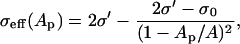
where σ₀ is the tension of the membrane without pores, σ′ is the energy per area of the hydrocarbon-water interface, , and A is the surface area of the cell. This study assumes that changes of cell area, volume, and shape can be ignored for millisecond pulses considered here.

Numerical implementation

The numerical solution of the governing Eqs. 1–3, 6, 7, and 9 is based on our previous studies (13,24). Briefly, the spherical cell of radius a is immersed in a spherical shell of extracellular fluid of thickness 2a. Both intra- and extracellular space are discretized using spherical coordinates; discretization steps are Δθ = π/128 and Δρ = 3a/60. Equation 1 governing potentials Φ_i and Φ_e are transformed using the finite difference method into a set of linear equations. The external electric field is imposed as a Dirichlet boundary condition on the potential Φ_e along the outer boundary of the extracellular shell (ρ = 3a) consistent with Eq. 2. Continuity of current across the membrane, given by Eq. 3, is imposed treating the values of current through electropores, , as known. (For a discretized cell, superscripts are used to distinguish membrane-related quantities that change with the polar angle from quantities that apply to the whole cell, which have no superscripts; see next subsection.) The resulting set of equations is solved at each time step, yielding potentials Φ_i and Φ_e. The transmembrane potential is computed by subtracting the value of Φ_e, taken at a node adjacent to the membrane, from the value of Φ_i on the opposite side of the membrane.

Next, for each discrete angle θ on the membrane, new values of the number of pores and their radii are computed. To speed up computations, the model keeps track of two distinct populations of pores. Small pores, whose radii congregate near the minimum-energy radius of ∼1 nm, are accounted for by the local pore density N^θ. All pores in this population are assumed to have the same radius , which evolves according to Eq. 9 with r_j replaced by . Large pores, whose radii are larger than , are represented individually: the radius of each pore evolves according to Eq. 9. The exchange of pores between these two populations proceeds as follows. Pores created according to Eq. 7 are all initially treated as large. Pores remain in the large pore population throughout the initial stage of creation and rapid expansion of pores. Afterward, pore growth slows down and eventually some pores start to shrink. If any large pore shrinks to within 1 pm of , it is absorbed into the small pore population, thereby increasing N^θ and decreasing the local number of large pores, . To make sure that the absorption of pores does not introduce artifacts, key simulations were repeated without pore absorption.

Equations 7 and 9 are solved using the midpoint implicit method. The updated vectors , N^θ, , and are used to compute the current through pores and the effective membrane tension σ_eff. The vector will be used in the next time step to determine Φ_i and Φ_e.

Three features of implementation aim at increasing computational efficiency. First, to limit the number of pore radii that need to be updated by solving Eqs. 9, pores created at the same time-step are treated as a group rather than individually. Second, having two distinct populations of small and large pores further limits the number of independently-evolving pore radii. For example, a 40 kV/m field creates 341,000 pores. All pores belong to the large pore population for only ∼2.5 μs; by 100 μs, all but 16,000 pores have been absorbed into the small pore population. Finally, the solution uses adaptive time-stepping. Initially, Δt = 1.5 ns is used to resolve very fast transients associated with the creation of pores. Once pore creation ends and the dependent variables change less rapidly, Δt is gradually increased to 0.1 μs. The above initial and final Δt yield mean errors in voltage and maximum pore radius <0.1%, and in pore density, below 4%. The simulation of a 1-ms, 40 kV/m pulse takes ∼5 min (model implemented in C and running on a 3.4 GHz Pentium 4 processor under CentOS 4.0).

Pore statistics

At a position specified by a polar angle θ, the electroporation process is characterized by the local quantities in Table 2. All these quantities have superscripts indicating their dependence on the polar angle. Five locations on the cell membrane are of particular interest (Fig. 1): the depolarized pole (D), hyperpolarized pole (H), equator (E), and borders between electroporated and nonelectroporating regions (D_b and H_b). Thus, the general superscript θ may be replaced by D, H, etc., indicating the specific location.

TABLE 2.

Local characteristics of electroporation

	Transmembrane potential.
	Number of all (small, large) pores within ΔA surface area associated with one node.
Nθ	Density of small pores ().
	Surface conductance of the membrane (in S/m2) due to all (small, large) pores.
	Fractional pore area due to all (small, large) pores, e.g., .
	Maximum local radius.
r̄θ	Average radius of large pores.

FIGURE 1.

Schematic of a spherical cell considered in this study. Locations of particular interest are indicated by labels: D (H), depolarized (hyperpolarized) pole, D_b (H_b), border between electroporated and nonelectroporated region in the depolarized (hyperpolarized) part of the cell, E, cell equator. An arrow indicates the direction of the electric field E, polar angle θ measures the position along the cell circumference.

In the entire cell, the electroporation process is characterized by the quantities in Table 3. These quantities do not have any superscripts, which indicates that they apply to the entire cell.

TABLE 3.

Characteristics of electroporation in the entire cell

K (Ksm, Klg)	Number of all (small, large) pores.
G (Gsm, Glg)	Conductance of the cell (in S) due to all (small, large) pores, e.g., .
F (Fsm, Flg)	Fractional pore area due to all (small, large) pores, e.g., .
rmax	Maximum radius anywhere on the cell.
r̄	Average radius of large pores.
θd (θh)	Polar angle of the border between electroporated and intact membrane on the depolarized (hyperpolarized) hemisphere.

RESULTS

Creation and time evolution of pores

Consider a 50-μm cell exposed to a 40 kV/m electric field for 1 ms. As seen in Fig. 2, the electroporation process can be divided into three distinct stages: charging, pore nucleation, and pore evolution (dotted vertical lines separate the stages).

FIGURE 2.

Time evolution of electroporation in a cell. (A) Transmembrane potential at the locations indicated by labels. (B) Number of all pores K^θ at locations D, H, and H_b. There is only one pore at H_b, no pores at D_b or E. K^θ of 10⁴ corresponds to a pore density of 4.07 × 10¹³ pores/m². (C) Radii of 12 selected pores at the depolarized pole. (D) Maximum radii at locations indicated by labels. The pore at location D_b was created at 0.32 ms. Note the different timescales in panels A and B versus C and D. Dotted vertical lines in panels A and B indicate the start and the end of the pore nucleation stage.

The charging stage starts with the application of the electric field and ends with the formation of the first pore anywhere on the cell membrane. Since the membrane does not yet contain any pores, current I_p in Eq. 3 is zero and the membrane charges like a parallel resistance and capacitance. This passive charging can be seen during the first 0.51 μs in Fig. 2 A, when transmembrane potential increases in magnitude from its initial value of V_rest = −0.08 V according to the formula

(12)

The charging phase ends at 0.51 μs, when the first pore is created. As expected, this pore appears on the hyperpolarized pole (H) of the cell: during charging, has larger magnitude than because of the negative V_rest.

Pore nucleation at a specific angle θ starts when its transmembrane potential exceeds a threshold value of ∼1 V. There is no sharp threshold for electroporation: as expected from Eq. 7, any V_m > 0 will create pores but weak pulses may require a very long time (41). Experiments typically use pulses up to milliseconds in duration, and electroporation is identified either by the uptake of small molecules (5,6) or by the decrease in V_m during the pulse (42–44). Using the latter criterion and assuming that a 5% decrease is experimentally detectable, the model's parameter V_ep was chosen so that V_m < 1 V will be considered subthreshold.

Locations where exceeds threshold experience a dramatic increase in the pore creation rate (Eq. 7), and hence the number of pores increases. These pores add additional pathways for current to cross the membrane, and thus increase its local conductance G^θ. In consequence, no longer follows the charging transient that would be observed in a cell with a passive membrane (Eq. 12). As seen in Fig. 2 A, the magnitude of peaks and then decreases.

Since different locations on the cell membrane reach threshold at different times, the timing and the degree of decrease depend on the position. As seen in Fig. 2 B, polar regions, D and H, begin the formation of pores the earliest, at 0.65 and 0.51 μs, and they accumulate 8.9 × 10³ and 10.1 × 10³ pores, respectively (the corresponding pore densities are 3.63 × 10¹³ and 4.11 × 10¹³ pores/m²). Consequently, D and H experience the largest decrease in the magnitude of : by the end of the pulse, ) discharges from a peak value of 1.34 V (−1.35 V) to 0.38 V (−0.36 V). In contrast, border locations, D_b and H_b, contain only one pore each (pore density of 4.07 × 10⁹ pores/m²), which were created at 1.5 μs at H_b, and as late as 0.32 ms at D_b. These locations still see a considerable drop in voltage magnitude, from just above ±1 V to 0.65 V (−0.59 V) at D_b (H_b). Interestingly, starts decreasing at 1.5 μs, even though the pore does not form at this location until much later. This example demonstrates that is strongly influenced by the state of the membrane in the adjacent regions and thus it decreases even in the regions of the cell membrane that are not electroporated.

The pore nucleation stage is assumed completed when the relative increase in the total number of pores per time step drops below 10⁻⁶. According to this definition, in the example of Fig. 2, nucleation ends at 1.43 μs. Even though a few pores may be created after this time (such as at the border regions D_b and H_b), the vast majority of pores are created within the time interval indicated by the dotted vertical lines in Fig. 2.

Pore evolution is a considerably slower process than either pore nucleation or changes in . Pores start growing immediately after they are created but their radii are no more than 5 nm by the end of the nucleation phase. Most of the pore evolution occurs after the creation of new pores has ceased and even after has leveled off, both of which happen within microseconds. In contrast, some pore radii will not reach steady state during the first millisecond of the 40 kV/m pulse (Fig. 2, C and D) and will continue to evolve, although subsequent changes will be relatively small. Since no longer changes, this adjustment of pore radii is driven by the last two terms of the advection velocity (Eq. 10): the line energy of pore perimeters and the effective tension of the membrane. The latter factor is especially significant: as pores grow, they relieve membrane tension, so the effective membrane tension σ_eff decreases (Eq. 11). Because σ_eff couples all pores on the cell, pores evolve to minimize not their individual energies but the energy of the entire membrane (30).

The minimization of the membrane energy is the driving factor behind the division of all pores into two populations. As illustrated in Fig. 2 C for the depolarized pole, all pores initially grow but soon smaller pores start shrinking and eventually assume a radius of ∼1 nm (membrane energy has a local minimum here). These form the population of “small” pores. Small pores are subject to resealing (Eq. 7). In experiments, resealing time is highly variable (39,45) but considerably longer than a 1-ms pulse considered here. In the model, the resealing time is on the order of seconds (with parameters of Table 1), so the small pores do not disappear during the pulse.

The remaining pores adjust their radii to a range of 15–25 nm, forming a population of “large” pores. Their radii are determined primarily by the local number of pores and local , with some impact from the number of pores on the entire cell. Thus, pore sizes vary with the position on the cell. Fig. 2 D shows the radii of the largest pore at locations D, H, D_b, and H_b (there are no pores at E). This figure illustrates the differences in both pore sizes and their rates of change between the polar and border regions of the cell.

Spatial distribution of transmembrane potential and pores

Voltage

Fig. 3 A shows how the transmembrane potential V_m changes along the cell circumference. Up to 0.51 μs, V_m maintains a cosinusoidal profile predicted by Eq. 12. By 1.43 μs, large dips develop in the V_m profile at the two polar regions of the cell. These dips are the direct consequence of the creation of pores in these regions. Because at this time all pores are still small and fairly uniform in size (dashed line in Fig. 3 C), the depth of the dips is related to the number of pores created at any particular location (heavy line in Fig. 3 B). This relation breaks down as pore radii evolve, and by 1 ms, becomes nearly flat in the electroporated regions of the cell. The magnitude of is larger near the border of the electroporated region, in which fewer pores provide fewer pathways for the transmembrane current.

FIGURE 3.

Spatial distribution of electroporation in a cell. (A) Transmembrane potential at times indicated in the legend. The dotted line is the steady-state potential that would have been achieved without electroporation. The times 0.51 and 1.43 μs are the start and the end of the pore nucleation stage. (B) Number of all pores K^θ and number of large pores at 1 ms. Note the 10-fold difference in scales for K^θ and . (C) Maximum radius at the end of the nucleation stage (1.43 μs) and at 1 ms. (D) Membrane conductance G^θ at the times indicated in the legend. In panels A–D, solid circles on the 1-ms plots indicate locations D, D_b, E, H_b, and H (left to right).

At 1 ms, transmembrane potential is at its steady state. Note that the nonelectroporated regions of the cell have magnitude considerably lower than they would in absence of electroporation (dotted line). It confirms that electroporation lowers the magnitude of not only locally in the regions where the pores are created but also throughout the entire cell.

Pores

Fig. 3 B shows the total number of pores K^θ as a function of position on the cell surface. It confirms that the decrease in seen in Fig. 3 A is a direct reaction to the creation of pores. There are no pores in the regions around the equator, 0.95 < θ < 2.17 rad (54° < θ < 124°), in which has never reached the electroporation threshold.

Of all existing pores, only a small fraction belong to the large pore population, as illustrated by the thin line in Fig. 3 B (in interpreting this figure, note that the scale for large pores is 10 times larger than the scale for the small pores). increases as one moves toward the border of the electroporated region: since fewer pores were created there, nearly all of them grow to compensate for their smaller number. As illustrated in Fig. 3 C, which shows the maximum pore radii, , at each location, some border-zone pores grow to very large sizes and exceed 300 nm. In contrast, the largest pores in the polar regions of the cell, where is flat, have radii of ∼23 nm (except near the hyperpolarized pole).

Membrane conductance

The interplay of the pore number and their sizes produces interesting changes in the conductance of the cell membrane (Fig. 3 D). The surface conductance G^θ has the largest value early in the electroporating process. For example, at 1.43 μs, when the pores have already been created but are still relatively small, G^D is 8.6 × 10⁴ S/m². A visible increase in G^θ is limited to the regions where a significant number of pores are created, i.e., closer to the poles and not in the border zone. As the pore radii evolve in time, the G^θ distribution decreases in magnitude and broadens. By 1 ms, G^D has dropped to 5.8 × 10⁴ S/m² and has increased from zero to 0.68 × 10⁴ S/m².

Distribution of pore radii

As seen in Fig. 2 C, pores divide themselves into two distinct populations: small pores, with radii close to 1 nm, and large pores, with radii well above 1 nm. Small pores greatly outnumber the large ones (see Fig. 4 for specific numbers). At 1 ms, 97.8% of all pores on a cell are small, and the remaining 2.2% are large. Despite their much greater number, small pores comprise only 4.7% of the total pore area and they contribute 34% to the increased conductance of the cell. In polar regions D and H, small pores play a larger role: 99% of pores at pole D are small, they comprise 19.5% of the local pore area, and account for over half (57.5%) of membrane conductance.

FIGURE 4.

Distribution of pore radii at 30 μs, 100 μs, and 1 ms. (A) Pores at the depolarized pole D. (B) Pores on the entire cell. Only large pores are included in the distributions and their number K_lg is given on each panel. The total number of pores, K, is reported in the upper panels. Two lower panels of panel B cover only part of the range of pore radii; maximum radii r_max are reported in each panel. The bin width = 2 nm.

The evolution of radii within the large pore population is illustrated in Fig. 4. At pole D, the number of large pores, , decreases with time while the distribution of pore radii moves toward larger values, reaching 19.4 ± 3.4 nm (mean and standard deviation) at 1 ms, with 90 large pores. The behavior of large pores depends on their location on the cell. In the polar regions, where is flat, pores behave similarly to the pores at the D pole: some shrink and become small, while others continue to grow. Pores from the border zones grow more vigorously to compensate for their much smaller number and reach radii up to 419 nm. However, at 1 ms only 91 pores (out of 7600 large pores) have radii above 100 nm. The average radius over all large pores is 22.8 ± 18.7 nm.

Postpulse transient

The electric pulse is terminated at 1 ms. Immediately, the cell membrane starts discharging and 2 μs later, drops to nearly zero. At 0.5 ms after the pulse, the cell is slightly hyperpolarized, with varying from −40 μV at the poles to −105 μV on the equator. In response to the drop in , pores start shrinking rapidly. Fig. 5 A shows the postpulse evolution of pore radii at location D (it is the continuation of pore evolution shown in Fig. 2 C). The large pore population disappears when all large pores have become so small that they are absorbed into the small pore population. This process lasts 15–20 μs, depending on the initial sizes of pores at a given position. This fast shrinkage should not be confused with resealing, which proceeds with a time constant of seconds. Thus, at 0.5 ms after the pulse, all pores are still present but their radii have shrunk to 0.8 nm (local energy minimum for V_m = 0).

FIGURE 5.

Postpulse evolution of the pores in a cell. The electric field has been turned off at 1 ms. (A) Radii of 12 selected pores (seven large and five small) at the depolarized pole D. This panel is a continuation of Fig. 2 C. (B) Membrane conductance G^θ at the end of the pulse (1 ms, thin line) and after the pulse (1.5 ms, thick line). Solid circles on the 1.5-ms plots indicate locations D, D_b, E, H_b, and H (left to right).

As a result of pore shrinkage, the fractional pore area decreases over 20-fold, from 0.069% to 0.003% of the cell membrane area. Likewise, membrane conductance decreases: e.g., G^D drops from 5.8 × 10⁴ to 2.4 × 10⁴ S/m². Fig. 5 B shows the distributions of G at the end of a 1-ms pulse and 0.5 ms after its termination. These two distributions differ in both magnitude and shape. In particular, the shape of the postpulse distribution directly reflects the local number of pores (seen in Fig. 3 B) since the differences in pore radii no longer exist.

Effects of a nonzero resting potential

The model assumes that a cell is initially at rest, with . As a result, the hyperpolarized half of the cell has a head start over the depolarized half as they charge toward the threshold. There are several consequences of this asymmetry.

First, pores in the hyperpolarized half of the cell are created earlier than they are in the depolarized half: the first pore is created at 0.51 μs at location H and at 0.65 μs at D (Fig. 2 B). has a larger peak at H (−1.35 V) than at D (1.34 V), which leads to 12% more pores (Fig. 2 B). This difference in the number of pores results in significant differences in pore evolution (Fig. 2 D) and eventually leads to the asymmetry in pore distribution.

At 1 ms, the region next to pole H has more pores but fewer of them are large pores: and . The 11 pores at H grow to larger radii () but this growth does not quite compensate for their smaller number. Membrane conductance G^θ is smaller on the hyperpolarized half of the cell, except very close to the border zone (Fig. 6 B). The transmembrane potential is quite similar in both hemispheres (Fig. 6 A). Small differences in reflect the differences in conductance G^θ, with having larger magnitude wherever G^θ is smaller.

FIGURE 6.

Asymmetry of the electroporation process. (A) Transmembrane potential over the depolarized and hyperpolarized hemispheres (overlaid). (B) Membrane conductance, G^θ, over the depolarized and hyperpolarized hemispheres (overlaid). In both panels, solid circles indicate the position of the pole D and the border D_b; open circles indicate the pole H and the border H_b.

Although not apparent in Fig. 6 A because of the scale, the cell equator E is slightly depolarized. Fig. 7 shows time evolution of in more detail. Starting from the rest potential at −0.08 V, reaches a peak of 0.039 V at 5.6 μs and then discharges monotonically to 0.021 V at 1 ms. This depolarized value at the equator results from the asymmetry in membrane conductance, specifically from being higher than . Postpulse, quickly drops to a very small hyperpolarized value of −105 μV.

FIGURE 7.

Transmembrane potential at the equator of the cell. The dashed line indicates V_m = 0.

Effects of pulse strength

The pore distribution depends on the strength of the electric field E applied to the cell, and the model is used to explore this dependence. Fig. 8 illustrates the effect of field strength on the number of pores, their average radius, the area of pores, cell conductance, and the extent of electroporation. The field E ranged from 13 kV/m (close to threshold) to 100 kV/m, and all data were collected at the end of a 1-ms pulse.

FIGURE 8.

Dependence of cell electroporation on field strength. All results were collected at the end of a 1-ms pulse and apply to the whole cell. (A) Number of all pores (K) and number of small (K_sm) and large (K_lg) pores. The lines corresponding to K and K_sm overlap. (B) Number of pores in large pore population shown on an expanded vertical scale. (C) Average radius () of the large pore population. The vertical bars indicate standard deviation. For clarity, the range of the field strengths was truncated to 50 kV/m; continues at the same level beyond 50 kV/m. (D) Total area of pores reported as a fraction of the cell surface area. (E) Total conductance of the cell membrane. (F) Extent of electroporation in the cell measured by the polar radii θ_d and θ_h. To facilitate comparison with θ_d, the figure plots π–θ_h. The lines labeled an-dep and an-hyp show the extent of electroporation estimated from Eq. 12 for the depolarized and hyperpolarized hemisphere, respectively. The legend in panel A applies also to panels B, D, and E. Dotted vertical line indicates the electric field of 40 kV/m, i.e., the default field-strength used throughout this article.

As expected, the number of pores increases with the pulse strength but, except for very weak pulses, this increase is due to the creation of small pores. In Fig. 8 A, curves representing all pores and small pores overlap and large pores appear to be a negligible fraction of all pores. As seen on the expanded vertical axis in Fig. 8 B, the number of large pores K_lg initially increases but for E above 40 kV/m, K_lg slightly decreases and then levels off at ∼7000 pores. Likewise, the average radius of large pores, , essentially levels off as the pulse strength increases: for E above 20 kV/m, stays between 20 and 25 nm (Fig. 8 C). Despite their limited number and size, large pores continue to contribute significantly to the fractional pore area F (Fig. 8 D) and to the increase in cell conductance G (Fig. 8 E). For pulses 20 kV/m and below, essentially all increase of F and G is due to large pores. However, as the pulse strength increases, the contribution of small pores increases, especially to G. At E = 100 kV/m, 81% of cell conductance is due to small pores.

Fig. 8 F shows the extent of electroporation, measured as the polar angle of the border nodes between electroporated and intact regions (θ_d and θ_h). Small fluctuations seen in the curves result from the discretization of the cell's circumference. The figure shows that the extent of electroporation is very similar in both hemispheres. There is some asymmetry that results from the negative rest potential: for E ≥ 20 kV/m, θ_h is larger; for weaker pulses, θ_d exceeds θ_h. The extent of electroporation grows with the pulse strength but at an increasingly slower rate.

Single cell versus membrane electroporation

In the past, several studies investigated electroporation in a uniformly polarized membrane patch, viewing it as a representation of a depolarized or hyperpolarized polar region of a single cell (13,15,23). Thus, the question arises to what extent electroporation of the membrane resembles electroporation of a single cell. Having previously developed a model of electroporating membrane (13), we have the tools to address this question. We have adjusted parameters of our membrane model to correspond to those of the cell and ran simulations for the range of pulse strengths corresponding to those in Fig. 8. The results indicate that electroporation in a membrane patch indeed closely resembles electroporation at the polar regions: the number of pores and their area agree within an order of magnitude. Number of pores grows with the pulse strength but in both cases, this growth is due to small pores. The average radius of large pores decreases with the pulse strength and levels off at 20–25 nm. Above 45 kV/m in the cell (3.75 V in the membrane), large pores disappear altogether and only small pores are being created.

However, neither polar regions nor the membrane patch reflects electroporation in the cell as a whole. In a patch, the number of large pores decreases to zero as pulse strength increases but in the cell, it levels off (Fig. 8 B). Finally, in a patch the large pore population becomes increasingly more compact for stronger pulses so that all large pores have essentially the same radius (13). This accumulation of pore radii also occurs at any single position on a cell. However, over the entire cell, we observe large dispersion of pore sizes, owing to local differences in the transmembrane potential and the number of pores (Fig. 4, A–C). This comparison demonstrates that the spatial interactions have nontrivial effects on the process of cell electroporation, and that the behavior of a membrane patch differs in a substantial way from that of the entire cell.

DISCUSSION

The model presented here allows us to study both temporal and spatial aspects of cell electroporation without prohibitive computational costs. This section evaluates how well the results of the model match experiments.

In evaluation of the model, one needs to keep in mind that this study cannot even attempt to reproduce quantitatively the results of any particular experiment: it is not possible to find in the literature all parameters required by the model for a single cell type. Some parameters have been chosen to match the study of Hibino et al. (44), who used potentiometric dyes to visualize the evolution of transmembrane potential during electroporation of sea urchin eggs. That study provided us with values of the cell radius, intracellular and extracellular conductivity, membrane conductance, and threshold for electroporation. Other parameters listed in Table 1 came from other sources, many of them from experiments on artificial lipid bilayers. Thus, differences between the results of experiments and our model are to be expected.

Voltage

The most detailed information on the electroporation process in a cell came from measurements of using voltage-sensitive fluorescent dyes obtained by Hibino et al. (44). Observation of changes in fluorescence over the cell circumference as electroporation progresses provided us with the spatial distribution of and the timescale of its evolution. The model reproduces quite well the transmembrane potential measured in this study. Just like as seen in the experiment, in the model evolves on the timescale of microseconds, with the magnitude exhibiting the saturation characteristic of electroporation. The spatial distribution of is also similar: in the polar regions of the cell settles at a uniform value of ∼±0.42 V and has a larger magnitude near the border of the electroporated region. In both the model and the experiment, pore formation occurs first at the hyperpolarized pole owing to the negative rest potential.

In the experiment of Hibino et al. (44), the values of in the depolarized hemisphere, and also to a smaller degree in the hyperpolarized one, decrease in magnitude during the entire 1-ms pulse. In consequence, the cell potential exhibits a slow, depolarizing drift. No such drift is seen in the model: after the first 3 μs, at the two poles changes very little (Fig. 2 A). The possible origin of this drift and its consequences on the assessment of the membrane conductance are discussed below.

Number and spatial distribution of pores

It is usually assumed that most pores are created at the poles of the cell and that the number of pores decreases to zero near the equator. The model confirms this assumption (Fig. 3 B), and supplies a previously unknown observation that pores are much larger on the border of the electroporated region than at the poles (Fig. 3 C). This prediction is confirmed indirectly by the shape of the profile measured by Hibino et al. (44). In Fig. 4 of their article, not only flattens at the poles but with time also develops dips. This shape is reproduced by the model (Fig. 3 A), but only when the pores are allowed to grow. Our previous cell models, in which pore radii were kept constant, could reproduce only very small dips (24,46).

The model predicts that the pulse creates more but smaller pores on the hyperpolarized hemisphere and fewer but larger pores on the depolarized hemisphere. This prediction agrees with the experiment of Tekle et al. (5), in which small molecules (ethidium bromide and Ca²⁺) entered predominantly through the hyperpolarized end, while larger ones (propidium iodide and ethidium homodimer) entered predominantly through the depolarized end.

Extent of electroporation

By imaging the uptake of propidium iodide, Gabriel et al. (6) have shown that the extent of the electroporated cell membrane increases with the pulse strength, and that the critical polar angle θ_c is slightly larger on the hyperpolarized hemisphere. The model agrees with this observation for field strengths above 20 kV/m; for weaker fields, θ_h is actually smaller than θ_d (Fig. 8). This experiment also demonstrates that cos θ_c has a linear dependence on 1/E. In the model, the fit to the straight line is better for θ_h than for θ_d (correlation coefficients are 0.989 and 0.962, respectively).

Some studies have used Eq. 12 for charging of a passive cell to evaluate which parts of the cell are electroporated (16–19). The underlying assumption is that wherever found from Eq. 12 exceeds threshold, the membrane will be electroporated. As seen in Fig. 8, which shows θ_d and θ_h together with their estimates from Eq. 12, this method overestimates the extent of electroporation by 20–32%, depending on the pulse strength. The reason for this discrepancy is that the creation of pores diminishes the magnitude of everywhere on the membrane, not only in the electroporated regions (Fig. 3 A). Thus, the cell never reaches predicted by Eq. 12, and consequently the extent of electroporation is smaller.

Distribution of pore radii

An interesting prediction of the model is the existence of two distinct pore populations, small and large, the former being more numerous and the latter contributing more to the total pore area. We are not aware of an experimental study that has confirmed this prediction. For example, the study of Chang and Reese, who used rapid-freezing electron microscopy to visualize the evolution of pores in red blood cells, could measure only pores with radii above 1 nm, so the small pore population was not seen (47). Nevertheless, this finding may aid in interpretation of experiments involving uptake of fluorescent molecules. Depending on their sizes, marker molecules may not permeate pores from both populations. In particular, DNA uptake was found to be most effective with weak pulses that exceed threshold only slightly (48–51). Since neither the number of large pores nor their area decreases substantially with pulse strength (Fig. 8, B and D), this finding can be related to the decrease in the average pore radius, (Fig. 8 C). For pulses above 20 kV/m, levels off just above 20 nm. Considering that the effective radius of DNA is 5–9 nm (52), 20 nm pores should allow DNA permeation but perhaps transport is not as efficient as with larger pores. Alternatively, transport may be sufficiently effective but long pulses required for the uptake (at least 1 ms (53,54)) increase the probability of cells dying. Possibly, this question can be resolved with real-time observations of DNA uptake (55).

The sizes of large pores measured by Chang and Reese (47) range from 20 to 120 nm, and this estimate is comparable with radii predicted by the model when a weak pulse of 15 kV/m is used (Fig. 8 C). However, there is an important difference: in the experiment, the pores were observed 40 ms after the pulse. The model predicts that by this time, all pores would have shrunk to the minimum-energy radius of ∼0.8 nm (Fig. 5 A). While some researchers consider the pores observed by Chang and Reese (56) to be hemolysis pores induced by cell swelling, large electropores growing in the absence of the induced V_m have been observed in our model (13,30). This so-called postshock coarsening occurs when the initial tension of the membrane is high and when a weak pulse creates a subcritical number of pores.

Postpulse pore shrinkage

As seen in Fig. 5 A, within microseconds after the pulse termination, all pores shrink to the minimum-energy radius r_m ≈ 0.8 nm, where they persist until resealing takes place. This shrinkage of pores explains the experimental observation that the permeable state is long-lived for small, but not large, molecules (54,57,58). It may also underlay the postpulse decrease in membrane conductance observed experimentally by Glaser et al. (39).

Fractional pore area and membrane conductance

The huge increase in membrane conductance G^θ caused by creation of pores makes it impossible for the cell to maintain its negative rest potential and hence the on the equator is very small. Thus, to assure that currents entering and leaving the cell balance, the conductances of both hemispheres should be equal, at least approximately. This indeed happens in the model: distributions of membrane conductances differ slightly (Fig. 6 B) but the total conductances are nearly equal: 0.468 and 0.455 mS for depolarized and hyperpolarized hemispheres, respectively. A study of Tekle et al. (59) concludes that the total area of pores at the two hemispheres could be quite similar even if there is asymmetry in pore number and their sizes. This conclusion clearly assumes that the area and conductance of pores are linearly related. In reality, the relationship between the pore area and conductance is strongly influenced by assumptions made in computing the current through a pore. Equation 5, which accounts for the decrease of the transpore voltage, predicts that pore conductance grows slower than linearly with the pore area. Thus, the model predicts different pore areas on the depolarized and hyperpolarized hemispheres (11.7 and 9.9 μm²), even though their total conductances are approximately equal. The pore areas on the two hemispheres would be somewhat different if Eq. 5 incorporated interactions between ions and the pore walls.

It is much harder to reconcile the model's prediction with the results of Hibino et al. (44), who have inferred from their optical measurements of that the membrane conductance G^θ is asymmetric: G^D exceeds G^H by a factor of approximately two. This asymmetry can be traced to a slow drift of toward more positive values, which leads to depolarization of a cell. As stated above, this drift is not reproduced by the model. We have tested two hypotheses regarding its origin.

First, the cell may slowly depolarize because the current flowing through pores changes intracellular concentrations. To test this hypothesis, we have replaced Eq. 5 for a current through a pore by an ion-specific current composed of Na⁺, K⁺, Cl⁻, and Ca²⁺ ions, and we have allowed intracellular concentrations of these ions to vary, using the methods described in our previous publication (46). The results demonstrate that the change of ionic concentrations affects the number and size of pores, but has very little effect on the distribution of either or G^θ. Most importantly, no slow depolarization of the cell is observed.

Second, the slow depolarization of a cell and the resulting asymmetry of G^θ may be an artifact of the experiment, such as dye bleaching or calibration of fluorescence signals. We have found out that the latter may offer a plausible explanation. Note from Fig. 7 that transmembrane potential on the cell equator has a small depolarized value, 0.021 V. An experimenter may easily ignore it and assume that is zero. Consequently, voltages computed from fluorescence will be shifted by 0.021 V: the magnitude of will be decreased in the depolarized hemisphere and increased in the hyperpolarized hemisphere. If the shifted is used to compute membrane conductance, then G^D will be 6.1 × 10⁴ S/m² and G^H will be 5.4 × 10⁴ S/m², i.e., the same type of asymmetry as reported by Hibino et al. (7,44). However, Hibino et al. stress that they have not used the assumption that is zero in processing their fluorescence data.

It is also possible that the slow depolarization of the cell may be due to factors not included in the model, such as exchange of charged molecules between the two monolayers of the membrane (60,61). However, conductivity estimates inferred from measurements made with voltage-sensitive dyes can now be independently verified. Recent development of microelectroporation devices has opened up a possibility of impedance measurements during electroporation of single cells (8). The model indicates that such measurements should be performed during the pulse to avoid large errors caused by the postpulse shrinking of pores. If impedance measurements are performed after the pulse with small, subthreshold pulses, then the measured G will reflect the membrane conductance seen in Fig. 5, which shows a postpulse G^θ that is considerably smaller than G^θ during the pulse.

Stages of electroporation

The stages of electroporation seen in the model closely resemble the steps of electropermeabilization identified by Teissié et al. based on experimental observations (56). The “induction step” corresponds to the charging and nucleation stages of the model, the “expansion step” corresponds to the pore evolution stage, the “stabilization step” corresponds to the postpulse shrinkage of pores, and the “resealing step” corresponds to the resealing of small pores described by Eq. 7 (not discussed in this article but demonstrated in our previous studies (13,24)). The only step not seen in the model is the “memory effect” that describes changes in the membrane and cell behavior persisting on the timescale of hours.

While some of the model's predictions still must be confirmed experimentally, the resemblance between the model's “stages” and “steps” of electroporation seen in experiments gives us a reason to believe that the single cell model presented here may be ready to provide theoretical support for real-life applications. For example, it can be used to design pulsing protocols. The model's ability to compute dynamically the size of pores and their distribution on the cell surface in response to a pulse of a given strength allows one to develop and test in silico protocols tailored to specific tasks: cell lysis, creation of large pores for DNA uptake or small pores for drug delivery, minimization of cell stress, etc. In addition, the model can relate the impedance signal measured in on-chip single cell electroporation devices to the underlying stages of the electroporation process. Thus, the model can provide a rational basis for extracting more information from the easily accessible impedance measurements.

References

- 1.Potter, H. 1988. Electroporation in biology: methods, applications, and instrumentation. Anal. Biochem. 174:361–373. [DOI] [PubMed] [Google Scholar]
- 2.Sukharev, S. I., V. A. Klenchin, S. M. Serov, L. V. Chernomordik, and Y. A. Chizmadzhev. 1992. Electroporation and electrophoretic DNA transfer into cells. The effect of DNA interaction with electropores. Biophys. J. 63:1320–1327. [DOI] [PMC free article] [PubMed] [Google Scholar]
- 3.Weaver, J. C., and Y. A. Chizmadzhev. 1996. Theory of electroporation: a review. Bioelectrochem. Bioenerg. 41:135–160. [Google Scholar]
- 4.Dev, S. B., D. P. Rabussay, G. Widera, and G. A. Hofmann. 2000. Medical applications of electroporation. IEEE Trans. Plasma Sci. 28:206–223. [Google Scholar]
- 5.Tekle, E., R. D. Astumian, and P. B. Chock. 1994. Selective and asymmetric molecular transport across electroporated cell membranes. Proc. Natl. Acad. Sci. USA. 91:11512–11516. [DOI] [PMC free article] [PubMed] [Google Scholar]
- 6.Gabriel, B., and J. Teissié. 1997. Direct observation in the millisecond time range of fluorescent molecule asymmetrical interaction with the electropermeabilized cell membrane. Biophys. J. 73:2630–2637. [DOI] [PMC free article] [PubMed] [Google Scholar]
- 7.Hibino, M., M. Shigemori, H. Itoh, K. Nagayama, and K. Kinosita. 1991. Membrane conductance of an electroporated cell analyzed by submicrosecond imaging of transmembrane potential. Biophys. J. 59:209–220. [DOI] [PMC free article] [PubMed] [Google Scholar]
- 8.Huang, Y., N. S. Sekhon, J. Borninski, N. Chen, and B. Rubinsky. 2003. Instantaneous, quantitative single-cell viability assessment by electrical evaluation of cell membrane integrity with microfabricated devices. Sensors Actuat. A. 105:31–39. [Google Scholar]
- 9.Pastushenko, V. F., Y. A. Chizmadzhev, and V. B. Arakelyan. 1979. Electric breakdown of bilayer lipid membranes: II. Calculations of the membrane lifetime in the steady-state diffusion approximation. Bioelectrochem. Bioenerg. 6:53–62. [Google Scholar]
- 10.Barnett, A., and J. C. Weaver. 1991. Electroporation: a unified, quantitative theory of reversible electrical breakdown and mechanical rupture in artificial planar bilayer membranes. Bioelectrochem. Bioenerg. 25:163–182. [Google Scholar]
- 11.Freeman, S. A., M. A. Wang, and J. C. Weaver. 1994. Theory of electroporation of planar bilayer membranes: predictions of the aqueous area, change in capacitance, and pore-pore separation. Biophys. J. 67:42–56. [DOI] [PMC free article] [PubMed] [Google Scholar]
- 12.Neu, J. C., and W. Krassowska. 1999. Asymptotic model of electroporation. Phys. Rev. E. 59:3471–3482. [Google Scholar]
- 13.Smith, K. C., J. C. Neu, and W. Krassowska. 2004. Model of creation and evolution of stable macropores for DNA delivery. Biophys. J. 86:2813–2826. [DOI] [PMC free article] [PubMed] [Google Scholar]
- 14.Weaver, J. C. 1994. Theory of electroporation. Adv. Chem. Ser. 235:447–470. [Google Scholar]
- 15.Joshi, R. P., and K. H. Schoenbach. 2000. Electroporation dynamics in biological cells subjected to ultrafast electrical pulses: a numerical simulation study. Phys. Rev. E. 62:1025–1033. [DOI] [PubMed] [Google Scholar]
- 16.Serša, G., M. Čemažar, D. Šemrov, and D. Miklavčič. 1996. Changing electrode orientation improves the efficacy of electrochemotherapy of solid tumor in mice. Bioelectrochem. Bioenerg. 39:61–66. [Google Scholar]
- 17.Saulis, G. 1993. Cell electroporation. Part 3. Theoretical investigation of the appearance of asymmetric distribution of pores on the cell and their further evolution. Bioelectrochem. Bioenerg. 32:249–265. [Google Scholar]
- 18.Neumann, E., S. Kakorin, I. Tsoneva, B. Nikolova, and T. Tomov. 1996. Calcium-mediated DNA adsorption to yeast cells and kinetics of cell transformation by electroporation. Biophys. J. 71:868–877. [DOI] [PMC free article] [PubMed] [Google Scholar]
- 19.Kotnik, T., and D. Miklavčič. 2006. Theoretical evaluation of voltage inducement on internal membranes of biological cells exposed to electric fields. Biophys. J. 90:480–491. [DOI] [PMC free article] [PubMed] [Google Scholar]
- 20.Pavlin, M., and D. Miklavčič. 2003. Effective conductivity of a suspension of permeabilized cells: a theoretical analysis. Biophys. J. 85:719–729. [DOI] [PMC free article] [PubMed] [Google Scholar]
- 21.Davalos, R. V., B. Rubinsky, and D. M. Otten. 2002. A feasibility study for electrical impedance tomography as a means to monitor tissue electroporation for molecular medicine. IEEE Trans. Biomed. Eng. 49:400–403. [DOI] [PubMed] [Google Scholar]
- 22.Puc, M., T. Kotnik, L. M. Mir, and D. Miklavčič. 2003. Quantitative model of small molecules uptake after in vitro cell electropermeabilization. Bioelectrochemistry. 60:1–10. [DOI] [PubMed] [Google Scholar]
- 23.Gowrishankar, T. R., and J. C. Weaver. 2003. An approach to electrical modeling of single and multiple cells. Proc. Natl. Acad. Sci. USA. 100:3203–3208. [DOI] [PMC free article] [PubMed] [Google Scholar]
- 24.DeBruin, K. A., and W. Krassowska. 1999. Modeling electroporation in a single cell. I: Effects of field strength and rest potential. Biophys. J. 77:1213–1224. [DOI] [PMC free article] [PubMed] [Google Scholar]
- 25.Stewart, D. A., T. R. Gowrishankar, and J. C. Weaver. 2004. Transport lattice approach to describing cell electroporation: use of a local asymptotic model. IEEE Trans. Plasma Sci. 32:1696–1708. [Google Scholar]
- 26.Gowrishankar, T. R., A. T. Esser, Z. Vasilkoski, K. C. Smith, and J. C. Weaver. 2006. Microdosimetry for conventional and supra-electroporation in cells with organelles. Biochem. Biophys. Res. Commun. 341:1266–1276. [DOI] [PubMed] [Google Scholar]
- 27.Joshi, R. P., Q. Hu, K. H. Schoenbach, and S. J. Bebe. 2002. Simulations of electroporation dynamics and shape deformations in biological cells subjected to high voltage pulses. IEEE Trans. Plasma Sci. 30:1536–1546. [Google Scholar]
- 28.Joshi, R. P., Q. Hu, and K. H. Schoenbach. 2004. Modeling studies of cell response to ultrashort, high-intensity electric fields—implications for intracellular manipulation. IEEE Trans. Plasma Sci. 32:1677–1686. [Google Scholar]
- 29.Hu, Q., S. Viswanadham, R. P. Joshi, K. H. Schoenbach, S. J. Beebe, and P. F. Blackmore. 2005. Simulations of transient membrane behavior in cells subjected to a high-intensity ultrashort electric pulse. Phys. Rev. E. 71:031914. [DOI] [PubMed] [Google Scholar]
- 30.Neu, J. C., and W. Krassowska. 2003. Modeling postshock evolution of large electropores. Phys. Rev. E. 67:1–12. [DOI] [PubMed] [Google Scholar]
- 31.Neu, J. C., K. C. Smith, and W. Krassowska. 2003. Electrical energy required to form large conducting pores. Bioelectrochem. Bioenerg. 60:107–114. [DOI] [PubMed] [Google Scholar]
- 32.Chernomordik, L. V., S. I. Sukharev, I. G. Abidor, and Y. A. Chizmadzhev. 1983. Breakdown of lipid bilayer membranes in an electric field. Biochim. Biophys. Acta. 736:203–213. [Google Scholar]
- 33.Sakuma, I., T. Haraguchi, K. Ohuchi, Y. Fukui, I. Kodama, J. Toyama, N. Shibata, and S. Hosoda. 1998. A model analysis of aftereffects of high-intensity DC stimulation on action potential of ventricular muscle. IEEE Trans. Biomed. Eng. 45:258–267. [DOI] [PubMed] [Google Scholar]
- 34.DeBruin, K. A., and W. Krassowska. 1998. Electroporation and shock-induced transmembrane potential in a cardiac fiber during defibrillation strength shocks. Ann. Biomed. Eng. 26:584–596. [DOI] [PubMed] [Google Scholar]
- 35.Ashihara, T., and N. A. Trayanova. 2004. Asymmetry in membrane responses to electric shocks: insights from bidomain simulations. Biophys. J. 87:2271–2282. [DOI] [PMC free article] [PubMed] [Google Scholar]
- 36.Sambelashvili, A. T., V. P. Nikolski, and I. R. Efimov. 2004. Virtual electrode theory explains pacing threshold increase caused by cardiac tissue damage. Am. J. Physiol. 286:H2183–H2194. [DOI] [PubMed] [Google Scholar]
- 37.Newman, J. 1966. Resistance for flow of current to a disk. J. Electrochem. Soc. 113:501–502. [Google Scholar]
- 38.Powell, K. T., E. G. Derrick, and J. C. Weaver. 1986. A quantitative theory of reversible electrical breakdown of bilayer membranes. Bioelectrochem. Bioenerg. 15:243–255. [Google Scholar]
- 39.Glaser, R. W., S. L. Leikin, L. V. Chernomordik, V. F. Pastushenko, and A. I. Sokirko. 1988. Reversible electrical breakdown of lipid bilayers: formation and evolution of pores. Biochim. Biophys. Acta. 940:275–287. [DOI] [PubMed] [Google Scholar]
- 40.Barnett, A. 1990. The current-voltage relation of an aqueous pore in a lipid bilayer membrane. Biochim. Biophys. Acta. 1025:10–14. [DOI] [PubMed] [Google Scholar]
- 41.Melikov, K. C., V. A. Frolov, A. Ahcherbakov, A. V. Samsonov, and Y. A. Chizmadzhev. 2001. Voltage-induced nonconductive and metastable pores in unmodified lipid bilayers. Biophys. J. 80:1829–1836. [DOI] [PMC free article] [PubMed] [Google Scholar]
- 42.Benz, R., and U. Zimmermann. 1980. Relaxation studies on cell membranes and lipid bilayers in the high electric field range. Bioelectrochem. Bioenerg. 7:723–739. [Google Scholar]
- 43.Powell, K. T., A. W. Morgenthaler, and J. C. Weaver. 1989. Tissue electroporation. Observation of reversible electrical breakdown in viable frog skin. Biophys. J. 56:1163–1171. [DOI] [PMC free article] [PubMed] [Google Scholar]
- 44.Hibino, M., H. Itoh, and K. Kinosita. 1993. Time courses of cell electroporation as revealed by submicroscopic imaging of transmembrane potential. Biophys. J. 64:1789–1800. [DOI] [PMC free article] [PubMed] [Google Scholar]
- 45.Bier, M., S. M. Hammer, D. J. Canaday, and R. C. Lee. 1999. Kinetics of sealing for transient electropores in isolated mammalian skeletal muscle cells. Bioelectromagnetics. 20:194–201. [DOI] [PubMed] [Google Scholar]
- 46.DeBruin, K. A., and W. Krassowska. 1999. Modeling electroporation in a single cell. II: Effects of ionic concentrations. Biophys. J. 77:1225–1233. [DOI] [PMC free article] [PubMed] [Google Scholar]
- 47.Chang, D. C., and T. S. Reese. 1990. Changes in membrane structure induced by electroporation as revealed by rapid-freezing electron microscopy. Biophys. J. 58:1–12. [DOI] [PMC free article] [PubMed] [Google Scholar]
- 48.Hama-Inaba, H., M. Takahashi, M. Kasai, T. Shiomi, A. Ito, F. Hanaoka, and K. Sato. 1987. Optimum conditions for electric pulse mediated gene transfer to mammalian cells in suspension. Cell Struct. Funct. 12:173–180. [DOI] [PubMed] [Google Scholar]
- 49.Rols, M.-P., C. Delteil, M. Golzio, P. Dumond, S. Cros, and J. Teissié. 1998. In vivo electrically mediated protein and gene transfer in murine melanoma. Nat. Biotechnol. 16:168–171. [DOI] [PubMed] [Google Scholar]
- 50.Gehl, J., and L. M. Mir. 1999. Determination of optimal parameters for in vivo gene transfer by electroporation, using a rapid in vivo test for cell permeabilization. Biochem. Biophys. Res. Commun. 261:377–380. [DOI] [PubMed] [Google Scholar]
- 51.Yoshizato, K., T. Nishi, T. Goto, S. B. Dev, H. Takeshima, T. Kino, K. Tada, T. Kimura, S. Shiraishi, M. Kochi, J.-I. Kuratsu, G. A. Hofmann, and Y. Ushio. 2000. Gene delivery with optimized electroporation parameters shows potential for treatment of gliomas. Int. J. Oncol. 16:899–905. [DOI] [PubMed] [Google Scholar]
- 52.Rybenkov, V. V., A. V. Vologodskii, and N. R. Cozzarelli. 1997. The effect of ionic conditions on the conformations of supercoiled DNA: I. Sedimentation analysis. J. Mol. Biol. 267:299–311. [DOI] [PubMed] [Google Scholar]
- 53.Klenchin, V. A., S. I. Sukharev, S. M. Serov, L. V. Chernomordik, and Y. A. Chizmadzhev. 1991. Electrically induced DNA uptake by cells is a fast process involving DNA electrophoresis. Biophys. J. 60:804–811. [DOI] [PMC free article] [PubMed] [Google Scholar]
- 54.Rols, M.-P., and J. Teissié. 1998. Electropermeabilization of mammalian cells to macromolecules: control by pulse duration. Biophys. J. 74:1415–1423. [DOI] [PMC free article] [PubMed] [Google Scholar]
- 55.Phez, E., C. Faurie, M. Golzio, J. Teissié, and M.-P. Rols. 2005. New insights in the visualization of membrane permeabilization and DNA/membrane interaction of cells submitted to electric pulses. Biochim. Biophys. Acta. 1724:248–254. [DOI] [PubMed] [Google Scholar]
- 56.Teissié, J., M. Golzio, and M.-P. Rols. 2005. Mechanisms of cell membrane electropermeabilization: a minireview of our present (lack of?) knowledge. Biochim. Biophys. Acta. 1724:270–280. [DOI] [PubMed] [Google Scholar]
- 57.Wolf, H., M.-P. Rols, E. Boldt, E. Neumann, and J. Teissié. 1994. Control by pulse parameters of electric field-mediated gene transfer in mammalian cells. Biophys. J. 66:524–531. [DOI] [PMC free article] [PubMed] [Google Scholar]
- 58.Satkauskas, S., M. F. Bureau, M. Puc, A. Mahfoudi, D. Scherman, D. Miklavčič, and L. M. Mir. 2002. Mechanisms of in vivo DNA electrotransfer: respective contributions of cell electropermeabilization and DNA electrophoresis. Mol. Ther. 5:133–140. [DOI] [PubMed] [Google Scholar]
- 59.Tekle, E., R. D. Astumian, W. A. Friauf, and P. B. Chock. 2001. Asymmetric pore distribution and loss of membrane lipid in electroporated DOPC vesicles. Biophys. J. 81:960–968. [DOI] [PMC free article] [PubMed] [Google Scholar]
- 60.Haest, C. W. M., D. Kamp, and B. Deuticke. 1997. Transbilayer reorientation of phospholipid probes in the human erythrocyte membrane. Lessons from studies on electroporated and resealed cells. Biochim. Biophys. Acta. 1325:17–33. [DOI] [PubMed] [Google Scholar]
- 61.Vernier, P. T., Y. Sun, L. Marcu, C. M. Craft, and M. A. Gundersen. 2004. Nanopulse-induced phosphatidylserine translocation. Biophys. J. 86:4040–4048. [DOI] [PMC free article] [PubMed] [Google Scholar]
- 62.Chambers, E. L., and J. de Armendi. 1979. Membrane potential, action potential and activation potential of eggs of the sea urchin, Lytechinus variegatus. Exp. Cell Res. 122:203–218. [DOI] [PubMed] [Google Scholar]
- 63.Hénon, S., G. Lenormand, A. Richert, and F. Gallet. 1999. A new determination of the shear modulus of the human erythrocyte membrane using optical tweezers. Biophys. J. 76:1145–1151. [DOI] [PMC free article] [PubMed] [Google Scholar]
- 64.Israelachvili, J. 1992. Intermolecular and Surface Forces, 2nd Ed. Academic Press, London, UK.